R E S E A R C H
Open Access
Iterative learning control for image feature
extraction with multiple-image blends
Yinjun Zhang
1,2, Yinghui Li
1*and Jianhuan Su
2Abstract
In this paper, a novel method of image extraction is proposed. Firstly, the image information is embedded into the parameters of the chaotic system, and then the image is overlapped and embedded to complete the image hiding. This process is equivalent to a dynamic system with unknown time-varying parameters. Secondly, the D-type iterative learning control algorithm is used to extract the information hidden in the image, because iterative learning can be used to estimate the time-varying parameter system completely in the time interval. Finally, the numerical simulation shows that the algorithm can effectively extract the hidden information under various attacks.
Keywords:Iterative learning control, Image extracting, Image hiding
1 Introduction
With the rapid development of Internet technology, it has provided great convenience for the dissemination of digital information products. On the other hand, copyright protection has become increasingly import-ant. Information hiding and digital watermarking as an important method of intellectual property protec-tion have attracted more and more attenprotec-tion.
In machine learning, in pattern recognition, and in image processing, feature extraction starts from an ini-tial set of measured data and builds derived values (fea-tures) intended to be informative and non-redundant, facilitating the subsequent learning and generalization steps, and in some cases, leading to better human in-terpretations. Feature extraction is related to dimen-sionality reduction.
When the input data to an algorithm is too large to be processed and it is suspected to be redundant (e.g., the same measurement in both feet and meters, or the repetitiveness of images presented as pixels), then it can be transformed into a reduced set of features (also named a feature vector). Determining a subset of the initial features is called feature selection [1]. The se-lected features are expected to contain the relevant in-formation from the input data, so that the desired task
can be performed by using this reduced representation instead of the complete initial data.
Feature extraction involves reducing the amount of resources required to describe a large set of data. When performing analysis of complex data, one of the major problems stems from the number of variables involved. Analysis with a large number of variables generally requires a large amount of memory and com-putation power; also, it may cause a classification algo-rithm to over fit to training samples and generalize poorly to new samples. Feature extraction is a general term for methods of constructing combinations of the variables to get around these problems while still de-scribing the data with sufficient accuracy. Many ma-chine learning practitioners believe that properly optimized feature extraction is the key to effective model construction.
One very important area of application is image pro-cessing, in which algorithms are used to detect and isolate various desired portions or shapes (features) of a digi-tized image or video stream. It is particularly import-ant in the area of optical character recognition.
Results can be improved using constructed sets of application-dependent features, typically built by an expert. One such process is called feature engineering. Alternatively, general dimensionality reduction tech-niques are used such as (1) independent component analysis, (2) Isomap, (3) kernel PCA, (4) latent se-mantic analysis, (5) partial least squares, (6) principal * Correspondence:[email protected]
1Aeronautics and Astronautics Engineering Institute, Air Force Engineering
University, Xi’an 710038, Shanxi Province, China
Full list of author information is available at the end of the article
component analysis, (7) multifactor dimensionality re-duction, (8) nonlinear dimensionality rere-duction, (9) multilinear principal component analysis, (10) multi-linear subspace learning, (11) semidefinite embedding, and (12) autoencoder.
Space technology [2, 3] and transform domain tech-nology [4,5] are the main methods of digital image hid-ing and embeddhid-ing. From the airspace algorithm point of view, the LSB (least significant bits) method is a typ-ical algorithm [6]. The method converts the spatial pixel values of the original carrier image from binary to decimalism and replaces each bit of information in the binary with the least significant bit in the correspond-ing carrier, and finally, the binary data containcorrespond-ing secret information is converted to decimal pixel, in order to regain the secret image. Although the method has good concealment, so that the human eye is difficult to de-tect, it has poor robustness.
The transform domain method is relatively stable, and the image hidden by the transform domain method has a certain resistance to image compression, filtering, rotation, shearing, and noise. Discrete cosine transform (DCT) [7], discrete Fourier transform (DFT) [8], and discrete wavelet transform (DWT) [9, 10] are
the main transform domain methods in recent years. We construct a unified form of the boundary value solving problem by constructing the matching func-tion, and finally, using the conventional spectral method to solve is an important method in the domain of transform domain [10]. In the process of exploring image-hiding algorithms, some scholars have proposed an iterative hybrid image-hiding encryption algorithm [11]. The main idea of the algorithm is to embed an image into another image. The image is repeatedly em-bedded into a set of image, accordingly to adjust the it-eration parameters to achieve the invisibility of the image. The algorithm provides a new way for better se-lection of the mixing parameters, but it shows weak robustness of the system due to the multiple product amplification of the mixed image change value. Due to the weak robustness caused by the error multi-amplifi-cation in [12], Urvoy [13] proposed an iterative hybrid algorithm for image modification that uses a partial image that does not contain a watermark to modify the image containing the watermark. Thus, we can elimin-ate the error from the image. However, in the face of random attacks such as Gaussian noise, the quality of the watermark we extract is poor. In order to improve
the stability of the watermarking system, the literature [14, 15] proposed JADE blind separation watermark-ing algorithm. This method used an iterative hybrid method to embed the image and used the hidden image and the carrier image as different signals. By separating the matrix to determine whether there is hidden information, there is no need to know the exact location of the embedded image. When the two signals that need to be separated have a strong correl-ation, the method cannot separate the related signals well.
In this paper, we proposed the image extraction method based on iterative learning algorithm, which is applied to the full estimation of time-varying parame-ters in finite time intervals under certain convergence conditions. For the repeated mixed images, a new image extraction method is proposed in this paper. It-erative learning identification technology is used to re-construct the image information signals. For the class of chaotic map and iterative hybrid encryption image system, an iterative learning identification law is con-structed. Under the conditions of given learning law and initial state of the system, the sufficient condi-tions for learning gain convergence are deduced, and the convergence of the system is proved. Using itera-tive learning identification method to estimate the time-varying parameters completely in finite time interval, we can achieve completely reconstruction of image informa-tion in digital image watermarking system.
Remarks: Here are some general mathematical sym-bols used in this paper. L2(Ω) (or short in L2)
repre-sents a kind of Ω function space consisted by all
measureable functions and it is bounded, satisfying up
¼ ( Z
Ω
juðxÞjpdx )1=p
<∞ ð1≤p≤∞Þ. Lp(Ω)is Banach space,L2(Ω) is Hilbert space.
For the n dimensional vector u¼ ðuT
1;uT2;⋯;uTi Þ,
where the norm of definition iskuk ¼
P
i¼1 n
u2i 1=2
. If
ui(x)∈L2, i= 1, 2, ⋯, n then Q(x) = (Q1(x),Q2(x),L,
Qn(x))∈Rn∩L2andkQkL2 ¼
( Z
Ω
ðQTðxÞQðxÞÞ2dx )1=2
.
For the function f(x,t) :Ω× [0,T]→Rn, f(gt)∈Rn∩L2, t∈[0,T], define its (L2,λ) norm as follows kfkðL2;λÞ
¼ sup
0≤t≤T n
kfk2L2
e−λt
o .
2 Digital image encryption
Chaotic cryptology includes two integral opposite parts: chaotic cryptography and chaotic cryptanalysis. Chaotic cryptography is the application of the math-ematical chaos theory to the practice of the cryptog-raphy, the study or techniques used to privately and securely transmit information with the presence of a third party or adversary. The use of chaos or random-ness in cryptography has long been sought after by en-tities wanting a new way to encrypt messages. However, because of the lack of thorough, provable security prop-erties and low acceptable performance, chaotic cryptog-raphy has encountered setbacks [1,16–18].
In order to use chaos theory efficiently in cryptog-raphy, the chaotic maps should be implemented such that the entropy generated by the map can produce re-quired confusion and diffusion. Properties in chaotic systems and cryptographic primitives share unique characteristics that allow for the chaotic systems to be applied to cryptography [19]. If chaotic parameters, as
Fig. 2Hidden image
well as cryptographic keys, can be mapped symmetric-ally or mapped to produce acceptable and functional outputs, it will make it next to impossible for an ad-versary to find the outputs without any knowledge of the initial values. Since chaotic maps in a real life sce-nario require a set of numbers that are limited, they may, in fact, have no real purpose in a cryptosystem if the chaotic behavior can be predicted. One of the most important issues for any cryptographic primitive is the security of the system. However, in numerous
cases, chaotic-based cryptography algorithms are
proved unsecure [17, 20–22]. The main issue in many of the cryptanalyzed algorithms is the inadequacy of the chaotic maps implemented in the system [23,24].
The concept of chaos cryptography or in the other words chaos-based cryptography can be divided into two major groups: the asymmetric [25, 26] and sym-metric [27–29] chaos-based cryptography. The major-ity of the symmetric chaos-based algorithms are based on the application of discrete chaotic maps in their process [27,30].
Bourbakis and Alexopoulos [31] in 1991 proposed
supposedly the earliest fully intended digital image en-cryption scheme which was based on SCAN language. Later on, with the emergence of chaos-based cryptog-raphy, hundreds of new image encryption algorithms, all with the aim of improving the security of digital images, were proposed [21]. However, there were three main aspects of the design of an image encryption that
was usually modified in different algorithms (chaotic map, application of the map, and structure of algo-rithm). The initial and perhaps the most crucial point was the chaotic map applied in the design of the algo-rithms [32–36]. The speed of the cryptosystem is always an important parameter in the evaluation of the efficiency of a cryptography algorithm; therefore, the designers were initially interested in using simple chaotic maps such as tent map, and the logistic map [19, 37]. However, in 2006 and 2007, the new image encryption algorithms based on more sophisticated chaotic maps proved that application of chaotic map with higher dimension could improve the quality and security of the cryptosystems [2,3,35,38,39].
In this paper, we use logistic encryption method to en-crypt the digital image. The logistic chaotic map is de-scribed as follows:
x tð þ1Þ ¼μx tð Þð1−x tð ÞÞ;x tð Þ∈ð0;1Þ ð1Þ
when 3.5699456⋯ ≤μ≤4, the unpredictability of the sequence x(t) generated by logistic chaotic maps. If the same initial value is given, a random sequence will be generated, under the mapping of the parameter A. If a different initial value is given, different data sequences will be generated, but the correlation between the data sequences is almost zero. The original image G is marked as θ(t). In order to achieve the invisibility of the image, we superpose and mix the known image sequence
Fig. 4Embedded carrier image and extracted hidden image
with the parameter μ, namely μ(t) =λ+θ(t); at the same time, the Eq. (1) can be written as
x tð þ1Þ ¼ðλþθð Þt Þx tð Þð1−x tð ÞÞ;x tð Þ∈ð0;1Þ ð2Þ
Thus, the chaotic sequence {x(t),t= 1,2,3,...} is the de-sired encrypted image G′, denoted here asx(t).
3 Method—multiple image blends
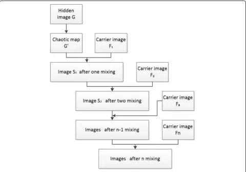
Assume that the image F is a pair of M × N digital im-ages, G′ needs to be hidden images, then a superim-posed mixed image S can be described as
S¼αFþð1−αÞG0 ð3Þ
α is adjustable mixing parameter, and F is carrier
image. S is an image sequence produced after a
super-position. According to Eq. (3), we know the 1−α
tends to 0, when mixing parameter α tends to 1, then the produced image sequence S=F. However, when the adjustable parameterαtends 0, the image sequence of superposition S will tend the hidden image G′. From the Eq. (3), we also know that when the value of the parameter α is closer to 1, the image G′ is hidden as much as possible. It is not easy to be detected, but it also increases the difficulty of the extraction.
Assume that the carrier images Fi(i= 1, 2,⋯,n) are different M × N digital images and the mixing parame-ters are αi∣αi∈[0, 1], i= 1, 2, ⋯, n. According to the
hybrid algorithm of image, firstly, we mix the image F1, G′, and α1 to get S1 =α1F1 + (1−α1)S1; secondly, we mix the image F2, G′, and α2 to get S2 =α2F2 + (1
−α2) G′, and so on. Finally, mix the images to get Sn =αnFn + (1−αn)Sn−1; Sn is called the digital image group which is a mixture of N images.
The mixed image satisfies the following relation:
S1ð Þ ¼t a1F1ð Þ þt ð1−a1Þx tð Þ S2ð Þ ¼t a2F2ð Þ þt ð1−a2ÞS1ð Þt
⋮
Snð Þ ¼t anFnð Þ þt ð1−anÞSn−1ð Þt 8
> > < > >
: ð
4Þ
so:
Sn¼αnFnþβnαn−1Fn−1þ⋯þβnβn−1⋯βn−iαn−iFn−i
þ⋯þβnβn−1⋯β2β1G 0
where βi= 1−αi, i= 1, 2, ⋯, n. When αitends to 1, the better the effect of watermark embedding, the worse the effect of watermark extraction. We use the logistic map to produce these iterative parameters. Selected param-eterμ′and initial valueα1.
αiþ1¼μ0αið1−αiÞ ð5Þ
According to Eq. (5), we can get a chaotic sequence
αi and use αi as the parameter sequence for each
image superposition and mixing. In order to avoid the correlation between the mixed images, the initial value α1 of the parameter μ′ in Eq. (5) cannot be the same as the parameter μ(t) and the initial value x(0) in Eq. (1).
Image encryption and its embedded process are shown in Fig.1.
4 The iterative learning control for image hidden with multi-blending
We use the image’s multiple hybrids embedding technol-ogy to embed image information into the time-varying pa-rameters of the digital image system and establish a mathematical model for the digital image system. The
Fig. 6Hidden image
image information is regarded as a finite time, and the it-erative learning identification method is applied to the image system. Variable parameters are estimated to achieve complete reproduction of image information.
We mark the initial image G asθ(t), then the encryp-tion image G′ as x(t) sequence. Carrier image group Fi(i= 1, 2,⋯,n) is ωiand the hybrid image Siisy(t); the system is described as
x tð þ1Þ ¼ f x tð ð Þ;θð Þt ;tÞ y1ð Þ ¼t h
1ðx tð Þ;tÞ y2ð Þ ¼t h2y1ð Þt ;t
⋯
ynð Þ ¼t hn yn−1ð Þt ;t
8 > > > > < > > > > :
ð6Þ
where t∈{0, 1, 2,⋯,N}, x(t)∈Rn, θ(t)∈R1, y1(t)∈R1, y(t)∈R1 are nonlinear function. f(x(t),θ(t),t) is the function of initial encryption image. The nonlinear function h1(x(t),t) represents an iterative mixed func-tion of the encrypted image and carrier image, and hn(yn−1(t),t) represents the mixed function of n iterations.
The iterative learning control system for estimating
θ(t) is:
xkðtþ1Þ ¼f xð kð Þt ;θkð Þt ;tÞ y1
kð Þ ¼t h1ðxkð Þt ;tÞ y2kð Þ ¼t h2y1kð Þt ;t
⋯
ynkð Þ ¼t hn yn−k 1ð Þt ;t
8 > > > > < > > > > :
ð7Þ
where k is iterative times and we use the same initial value. We suppose there exist f partial derivative Ak(t),
Bk(t) aboutx,θ,h1partial derivativeCk(t) aboutxandhi partial derivativeDki(t) abouty.
We use the D-type learning law:
θkð Þ ¼t satðϑkð Þt Þ
ϑkþ1ð Þ ¼t satðϑkð Þt Þ þL tð Þ h
ekðtþ1Þ−ekð Þt i (
ð8Þ
where sat(∙) is the saturation function,L(t) is the learning gain, andekðtÞ ¼yn−ynk.
Theorem 1 For the system (7) and learning law, if there exist
1
k −L tð ÞYn
i¼2Dkiðtþ1ÞCkðtþ1ÞBkð Þt k≤ρ<1 ð9Þ
then when k→∞, θ(t) converges to θk(t) interval {0, 1,⋯, N}.
Fig. 8Embedded carrier image and extracted hidden image
Proof
Remarkδxk(t) =xd(t)−xk(t),δθk(t) =θd(t)−θk(t)
δxkð Þ ¼t f xð dðt−1Þ;θdðt−1Þ;t−1Þ−f xð kðt−1Þ;θkðt−1Þ;t−1Þ þf xð dðt−1Þ;θkðt−1Þ;t−1Þ−f xð dðt−1Þ;θkðt−1Þ;t−1Þ
According to the differential mean value theorem, we have
f xð dðt−1Þ;θdðt−1Þ;t−1Þ−f xð kðt−1Þ;θkðt−1Þ;t−1Þ
¼Akðt−1Þδxkð Þt f xðdðt−1Þ;θdðt−1Þ;t−1Þ−f xð dðt−1Þ;θkðt−1Þ;t−1Þ
¼Bkðt−1Þδθkð Þtδxkð Þ ¼t Akðt−1Þδxkðt−1Þ þBkðt−1Þδθkðt−1Þ
ð10Þ
Taking the norm of Eq. (9)
δ
k xkð Þt ≤ctAkδxkð Þ þ0 k ct−A1cBkδθkð Þ þ0 k cAt−2cBkδθkð Þ1
þ
k ⋯þcBkδθkðt−1Þ
ð11Þ
Because the initial state is the same at each iteration,
δxk(0) = 0. The (10) can be written δ
k xkð Þt k≤ Xt−1
j¼0c t−j−1
A cBkδθkð Þkj ð12Þ
Multiplied by the two sidesc−λAt, yields
δxkð Þt
k kλ≤supXtj¼−1
0 cBc
t−j−1
A c−Aλtkδθkð Þjk
≤ cB cA cλA−1−1
ð13Þ
Supposec> maxfcA;1g, yields
δxkð Þt
k kλ≤ cB
cAðcλ−1−1Þ δθk t
ð Þ
k kλ ð14Þ
By (8), we have
δϑkþ1ð Þ ¼t δθkð Þt −L tð Þðekðtþ1Þ−ekð Þt Þ
¼δθkð Þt −L tð Þ ("
hn
yn−1ððtþ1Þ;tþ1
−hnyn−k 1ðtþ1Þ;tþ1 #
−
"
hnðyn−1ðð Þt ;tÞ
−hnyn−k 1ð Þt ;tÞ #)
ð15Þ
Remark
Akð Þ ¼t ∂
f xð kð Þt ;θkð Þt ;tÞ
∂xdð Þt
jxkð Þ ¼t ξkð Þt
whereξk(t) = (1−σ3)x(t) +σ3xk(k), 0 <σ3< 1 Bkð Þ ¼t ∂
f xð kð Þt ;θkð Þt ;tÞ
∂θkð Þt jθk t
ð Þ ¼ηkð Þt
whereηk(t) = (1−σ4)x(t) +σ4xk(k), 0 <σ4< 1
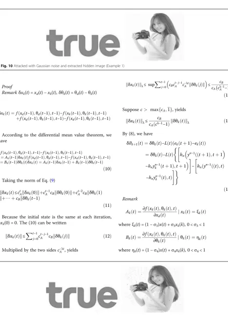
Fig. 10Attacked with Gaussian noise and extracted hidden image (Example 1)
DknðtÞ ¼∂hnðy∂y;tÞjy¼ξknðtÞ
whereξkn(t) = (1−σn)yn−1(t) +σnyn−1(t), 0 <σn< 1 hnðyn−1ððtþ1Þ;tþ1Þ−hn yn−k 1ðtþ1Þ;tþ1
¼Dknðtþ1Þðhn−1ðyn−2ððtþ1Þ;tþ1Þ−hn−1
yn−k 2ðtþ1Þ;tþ1
ð16Þ
hn yn−1ð Þt ;t
−hn yn−k 1ð Þt ;t
¼Dknð Þðt hn−1
yn−2ððtþ1Þ;tþ1Þ−hn−1
yn−k 2ð Þt ;t
ð17Þ
δϑkþ1ð Þ ¼t δθkð Þt −L tð Þ½ Qn
i¼2Dkiðtþ1ÞCkðtþ1ÞBkð Þt
f xð dð Þt ;θdð Þt ;tÞ−f xð kð Þt ;θkð Þt ;tÞ−
Yn
i¼2Dkið Þt Ckð Þt
δxkð Þt
ð18Þ
By definition ofAk(t) andBk(t), (18) can be written
δϑkþ1ð Þ ¼t 1−L tð Þ
Yn
i¼1Dkiðtþ1ÞCkðtþ1ÞBkð Þt
h i
δθkð Þt −L tð Þ Yn
i¼1Dkið Þt Ckð Þt−
Yn
i¼1Dkiðtþ1ÞCkðtþ1ÞAkð Þt
h i
δxkð Þt
ð19Þ
From Eq. (7), we have
δϑkþ1ð Þ ¼t ρδθkð Þ þt L Yn
i¼1Dkið Þt Ckð Þ−t Yn
i¼1Dkiðtþ1Þ
Ckðtþ1ÞAkð Þt
δxkð Þt
ð20Þ
Remark
MkðtÞ ¼L Q i¼1
n
DkiðtÞCkðtÞ−Q i¼1
n
Dkiðtþ1ÞCkðtþ1ÞAkðtÞ
So (19) can be written
δϑkþ1ð Þ ¼t ρδθkð Þ þt Mkð Þt δxkð Þt ð21Þ
SupposeMk(t)≤M, we takeλnorm of (21). δϑkþ1ð Þt
λ≤ρ δθk kð Þt kλþMkδxkð Þt kλ ð22Þ
Introducing (14) into (22), yields
δϑkþ1ð Þt
λ≤ρ δθk kð Þt kλþc McB Aðcλ−1−1Þ δθk
t
ð Þ
k kλ
ð23Þ
If there exist enoughλ, then lim
k→∞kδθkðtÞkλ¼0
The steps of using an iterative learning method to re-produce the hidden images are as follows:
1. We find the superimposed mixed imagey(t), and the initial estimateθ0(t) with the given arbitrary image sequence of multiple carrier wi(t) (i= 1,2,…,n), where
t∈{1, 2, ,N}.
2. Set initial statexk(0) =x0, substitutingθk(t) into the iterative learning control system, and obtain Sk(t) by solving.
3. Calculate the output error ek(t).
4. Using the iterative learning law to calculateθk+ 1(t). 5. The given error Jk¼ supt∈f0;1;2;⋯NgkδθkðtÞk, if
ek(t) < Jk, then the system will stop iteration; otherwise, setk=k+ 1, go to step 2).
The image information is hidden in time-varying par-ameter θk(t) obtained by the iterative learning method. A set of image sequences is known, and then the hid-den images are restored according to the pixel ratio of the image.
5 Results and discussions
For mixed images and restored hidden images, we can use the peak signal-to-noise ratio PSNR and normalized cross-correlation coefficient NC to measure the object-ive fidelity of the image. The peak signal-to-noise ratio of the original carrier image F and image S containing hidden information is measured.
PSNR is:
PSNR¼101g MN255
2
PM
i¼1
PN
j¼1ðFð Þi;j−Sð Þi;j Þ 2
!
ð24Þ
The peak signal-to-noise ratio PSNR is used as a measure of the objective fidelity of the image. The larger the value, the higher the fidelity of the image mixture.
Normalized cross correlation (NC) measures the de-gree of similarity between the extracted image and the original image. It is defined as:
Table 1Adding the Gaussian noise attack with Example 1
Gaussian noise VGN = 0.001 VGN = 0.01 VGN = 0.02
NC 0.9935 0.9781 0.9680
PSNR 25.673 24.823 22.081
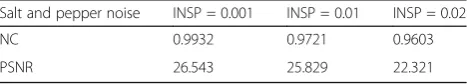
Table 2Adding the salt and pepper noise attack with Example 1
Salt and pepper noise INSP = 0.001 INSP = 0.01 INSP = 0.02
NC 0.9932 0.9721 0.9603
NC¼
PMM
iP¼1 x tð Þ ^x tð Þ MM i¼1 x tð Þ
2 ð25Þ
where x(t) and ^xðtÞ denote pixel value sequence of the original image and pixel value sequence of extracted image.
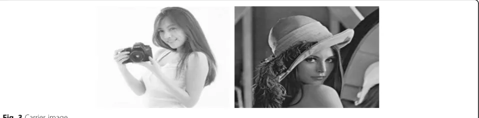
In this experiment, we use Camera (256*256) and Lena (256*256) as the two carrier images, and the binary image“true”(32*32) as the image to be hidden.
The state of the digital image embedding system is as follows:
xðtþ1Þ ¼ ðλþθðtÞÞxðtÞð1−xðtÞÞ y1ðtÞ ¼α1w1ðtÞ þ ð1−α1ÞxðtÞ
y2ðtÞ ¼α2w2ðtÞ þ ð1−α2Þy1ðtÞ
yðtÞ ¼y2ðtÞ 8
> > < > > :
Example 1. In the experiment, the hidden image
“true” is first embedded in the carrier image Lena. Then, the mixed image is embedded into the carrier image Camera again, and finally we obtain the mix-ture images. Taking λ= 3.568, the initial xk(0) = 0.5. Original image θ(t) is binary image, the carrier image w1(t) and w2(t) are two pixel points of the same gray image, and the images obtained after two times of superposition and mixing are y (t).
Takingλ= 3.568,α1= 0.52, according to the chaotic se-quence generated by the Eq. (5), {αi}, we choose the re-quired experimental parameter sequence {α1,α2}., the given learning gain is:
LkðtÞ ¼ðβ1β2ÞxkðtÞð1 1−xkðtÞÞ
whereβi= 1−αi,i= 1, 2
Figure 2 is the hidden image “true” used during the
experiment, and Fig. 3 is the carrier image Camera
and Lena. Firstly, the hidden image “true” needs to be embedded in the first carrier image Lena, and then the resulting mixed image is further embedded into the second carrier image Camera. Figure 4 is the final mixed image Camera and extracted hidden image using an iterative learning method. Experimental re-sults show that this method can completely recover hidden images.
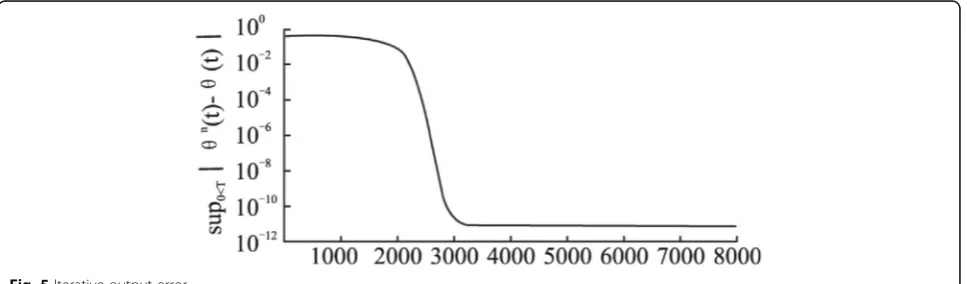
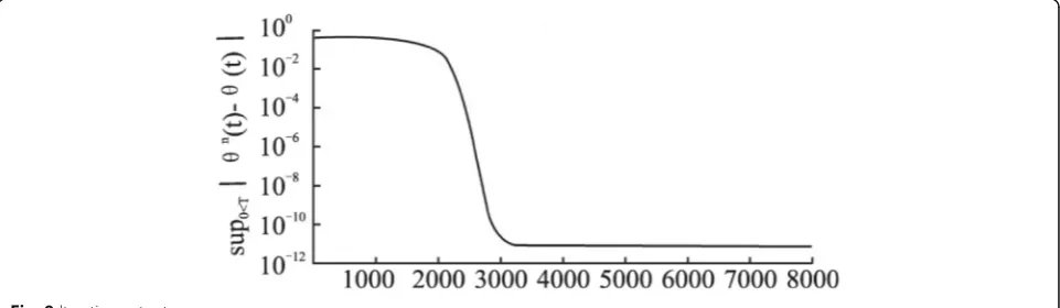
To verify the performance of the algorithm, we define the index function as
Jk¼ sup t∈f1;2;⋯;Ng
δθkð Þt
j j
We reconstruct the error convergence process of hidden image “true” by iterative learning algorithm. From Fig. 5, it can be seen that when the iterative times reach to 3000, the identified image and original image error has reached 10−12. The experimental re-sults show that the method effectively reconstructs the finite length information.
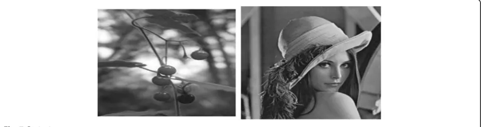
Example 2. In the experiment 2, the “wrong” is hid-den image. Cherry and Lena are carrier images, then we take the hidden image embeds into the carrier im-ages and obtain the mixture imim-ages finally. Taking λ= 4.256, the initial xk(0) = 0. The rest of the conditions are the same as the Example 1.
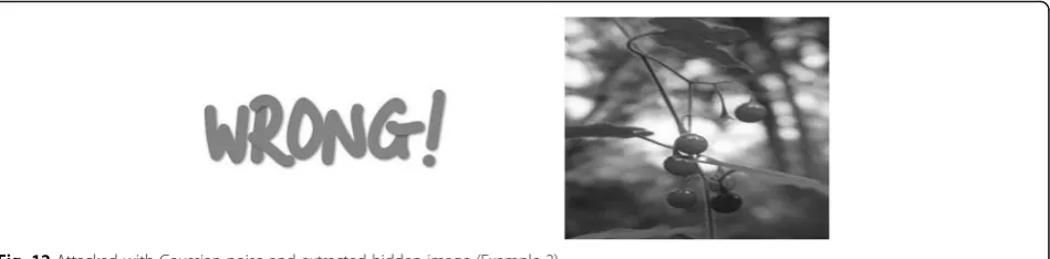
Fig. 12Attacked with Gaussian noise and extracted hidden image (Example 2)
By the chaotic sequence produced by Eq. (5), {αi}, the required experimental parameter sequences that we choose are {α1,α2} and the given learning gain is:
LkðtÞ ¼ðβ1β2ÞxkðtÞð1 1−xkðtÞÞ
whereβi= 1−αi,i= 1, 2
Figure6 is the hidden image “wrong”used during the experiment, and Cherry and Lena are the carrier images in Fig. 7. Firstly, we embed the “wrong” image into the Cherry and obtain a mixed image. Secondly, we embed the mixed image into the Lena image. Figure 8 is the final mixed image Cherry and extracting hidden image by the iterative learning way. Experimental results illus-trate that the way that we use can completely recon-struct the hidden image.
We use the same index function as experiment 1:
Jk¼ sup t∈f1;2;⋯;Ng
δθkð Þt
j j
We use the same algorithm to reconstruct the conver-gence process of hidden image“wrong.”We know the it-erative error has reached 10–14 with the iterative times reach to 3000 from Fig.9. The simulation shows the al-gorithm can effectively reconstruct the finite length information.
The anti-attack results of the test algorithm are as follows:
1. Anti-attack test adding Gauss noise and salt and pepper noise
Adding Gauss noise and salt and pepper noise to the mixed image, the Gauss noise variance VGN is 0.001, 0.01, and 0.02, respectively. Noise intensity of salt and pepper (INSP) is 0.001, 0.01, and 0.02.
Figures10and11show the mixed image and the
ex-tracted image after the attack. The similarity NC between the original image and the extracted image after the attack are shown in Table1. The peak signal-to-noise ratio PSNR of the original mixed image and the mixed image after the attack is shown in Table2.
2. Anti-attack test with compressed
The JPEG image compression method is a compres-sion attack for the mixed image. The smaller the com-pression factor Q, the higher the compression, that is, the greater the pixel loss. In Experiment 1 and Experi-ment 2, we separately select different compression fac-tors Qto extract the hidden images respectively. When Q= 10, the compression ratio is already very large. From Figs. 10, 11, 12, and 13, it can be seen that the “true” image proposed by the iterative learning identification method still has a high correlation NC (0.78) and better PSNR. It shows that the algorithm has better robustness for JPEG compression attack. The robustness of algorithms for JPEG compression attack are shown in (Tables3and4).
6 Conclusions
In this paper, we proposed the image extraction problem by using iterative learning algorithm. This method is to embed the hidden image into several different carrier images. Finally, the iterative learning is used to fully track the parameters of the image information, and the hidden image is reproduced. The parameters of the iterative learning law are updated with the change of time, which shows that the algorithm has better self-adaptability. Both experimental results show that when the mixed image with hidden information is attacked, the iterative learning recognition method can still recover the hidden image, and the ordinary reversible image solving method cannot restore the hidden image. The experimental data also proves the anti-attack of the algorithm.
Abbreviations
INSP:Noise intensity of salt and pepper; NC: Normalized cross correlation; PSNR: Peak signal to noise ratio; VGN: Gauss noise variance
Acknowledgements
The authors thank the editor and anonymous reviewers for their helpful comments and valuable suggestions.
Funding
The work was supported by the Hechi University Foundation (XJ2016ZD004), Hechi University Youth Teacher Foundation (XJ2017QN08), the Projection of Environment Master Foundation (2017HJA001, 2017HJB001), the important project of the New Century Teaching Reform Project in Guangxi (2010JGZ033), and Guangxi Youth teacher Foundation (2018KY0495).
Availability of data and materials
We can provide the data.
Authors’contributions
All authors contributed equally and significantly in writing this article. All authors read and approved the final manuscript. Yinghui Li is the corresponding author.
Authors’information
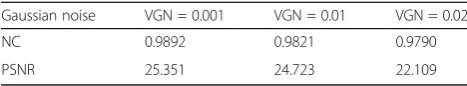
Yingjun Zhang was born in Xinjiang in 1984. He received the M.S. degree in control theory and control engineering from Guangxi Technology University in 2011. He is pursuing the Ph.D. in Air Force Engineering University. His research interests are in fault diagnosis control and iterative learning control. Table 3Adding the Gaussian noise attack with Example 2
Gaussian noise VGN = 0.001 VGN = 0.01 VGN = 0.02
NC 0.9892 0.9821 0.9790
PSNR 25.351 24.723 22.109
Table 4Adding the salt and pepper noise attack with Example 2
Salt and pepper noise INSP = 0.001 INSP = 0.01 INSP = 0.02
NC 0.9895 0.9801 0.9721
Yinghui Li (corresponding author) was born in Guangxi in 1966. She received the Ph.D. from Shanghai JiaoTong University. Now she is a professor in Air Force Engineering University. Her research interests include nonlinear control, motor control, and dynamics control.
Jianhuan Su was born in Guangxi in 1967. He received the M.S. from Chongqin University. Now he is a professor in Hechi University. His research interests include single process, nonlinear control.
Ethics approval and consent to participate
Approved.
Consent for publication
Approved.
Competing interests
The authors declare that they have no competing interests. And all authors have seen the manuscript and approved to submit to your journal. We confirm that the content of the manuscript has not been published or submitted for publication elsewhere.
Publisher’s Note
Springer Nature remains neutral with regard to jurisdictional claims in published maps and institutional affiliations.
Author details
1Aeronautics and Astronautics Engineering Institute, Air Force Engineering
University, Xi’an 710038, Shanxi Province, China.2School of Physics and Electrical Engineering, Hechi University Yizhou, No.42 Rd. Longjiang, Yizhou 546300, Guangxi, China.
Received: 13 July 2018 Accepted: 14 September 2018
References
1. E. Alpaydin,Introduction to Machine Learning(The MIT Press, London, 2010), p. 110 ISBN 978-0-262-01243-0. Retrieved 4 Feb 2017
2. Akhshani A, Mahmodi H, Akhavan A.A Novel Block Cipher Based on Hierarchy of One-Dimensional Composition Chaotic Maps[C]//. IEEE International Conference on Image Processing. IEEE, (Chicago, USA, 2007), pp. 1993-1996
3. Xie, Eric Yong, et al.On the cryptanalysis of Fridrich's chaotic image encryption scheme[J].Signal Processing.132(2), 150-154 (2017) 4. M.D. Swanson, Multimedia data-embedding and watermarking
technologies. Proc. IEEE86(6), 1064–1087 (1998)
5. J. Zhao, E. Koch, A generic digital watermarking model. Comput. Graph.
22(4), 397–403 (1998)
6. M.S. Fu, O.C. Au, Data hiding watermarking for halftone images. IEEE Trans. Image Process.11(4), 909–930 (2002)
7. W. Bender, D. Gruhl, Techniques for data hiding. IBM Syst. J35(4), 313–336 (1996)
8. C.H. Lee, Y.K. Lee, An adaptive digital image watermarking technique for copyright protection. IEEE Trans. Consum. Electron.45(4), 1005–1015 (1999) 9. N. Nikolaidis, I. Pitas, Robust image watermarking in the spatial domain.
Signal Process66(3), 385–403 (1998)
10. H.-p. Hu, L. Shuang-hong, Z.-x. Wang, A method for generating chaotic key stream. Chinese J Comput7(3), 408–414 (2004)
11. Liu R Z, Tan T N. Watermarking for digital images[C]//. International Conference on Signal Processing.2, 944-947 (2002)
12. M.A. Suhail, Digital watermarking-based DCT and JPEG model. IEEE Trans. Instrum. Meas.52(5), 1640–1647 (2003)
13. M. Urvoy, Perceptual DFT watermarking with improved detection and robustness to geometrical distortions. IEEE Trans. Inf. Forensics Secur.9(7), 1108–1119 (2014)
14. Y. Ishikawa, Optimization of size of pixel blocks for orthogonal transform in optical watermarking technique. J. Disp. Technol8(9), 505–510 (2012) 15. Y. Xu, S. Dong, B. Xuhui, Zero-error convergence of iterative learning control
using quantized error information. IMA J. Math. Control. Inf.34(3), 1061– 1077 (2016)
16. Y. Chen, X. Liao, Cryptanalysis on a modified Baptista-type cryptosystem with chaotic masking algorithm. Phys. Lett. A342(5–6), 389–396 (2005)
17. E.Y. Xie, C. Li, S. Yu, J. Lü, On the cryptanalysis of Fridrich’s chaotic image encryption scheme. Signal Process.132, 150–154 (2017)
18. A. Akhavan, A. Samsudin, A. Akhshani, Cryptanalysis of an improvement over an image encryption method based on total shuffling. Opt. Commun.
350, 77–82 (2015)
19. A. Akhavan, A. Samsudin, A. Akhshani, Cryptanalysis of an image encryption algorithm based on DNA encoding. Opt. Laser Technol95, 94–99 (2017) 20. M.S. Baptista, Cryptography with chaos. Phys. Lett. A240(1–2), 50–54 (1998) 21. S. Li, X. Zheng, Cryptanalysis of a chaotic image encryption method. 2002
Proc. IEEE Int. Symp. Circuits Syst. Proceedings (Cat. No.02CH37353). 2: II– 708–II–7112, 708–711 (2002)
22. G. Alvarez, S. Li, Some basic cryptographic requirements for chaos-based cryptosystems. Int. J. Bifurcation Chaos16(8), 2129–2151 (2006) 23. E. Solak, C. Çokal, O.T. Yildiz, T. Biyikoğlu, Cryptanalysis of Fridrich’s chaotic
image encryption. Int. J. Bifurcation Chaos20(5), 1405–1413 (2010) 24. Kwok H S, Tang W K S.A fast image encryption system based on chaotic
maps with finite precision representation[J]. Chaos Solitons & Fractals.32(4), 1518-1529 (2007)
25. C. Li, Cracking a hierarchical chaotic image encryption algorithm based on permutation. Signal Process.118, 203–210 (2016)
26. L. Kocarev, M. Sterjev, A. Fekete, G. Vattay, Public-key encryption with chaos. Chaos: an interdisciplinary. J. Nonlinear Sci.14(4), 1078–1082 (2004) 27. L. Kocarev, J. Makraduli, P. Amato, Public-key encryption based on Chebyshev
polynomials. Circuits Systems Signal Process24(5), 497–517 (2005) 28. A. Akhavan, A. Samsudin, A. Akhshani, A symmetric image encryption
scheme based on combination of nonlinear chaotic maps. J. Franklin Inst.
348(8), 1797–1813 (2011)
29. Y. Mao, G. Chen,Handbook of Geometric Computing(Springer, Heidelberg, 2005), pp. 231–265
30. S. Behnia, A. Akhshani, H. Mahmodi, A. Akhavan, A novel algorithm for image encryption based on mixture of chaotic maps. Chaos Solitons Fractals35(2), 408–419 (2008)
31. S. Behnia, A. Akhshani, H. Mahmodi, A. Akhavan, Chaotic cryptographic scheme based on composition maps. Int. J. Bifurcation Chaos.18(1), 251– 261 (2008)
32. N. Bourbakis, C. Alexopoulos, Picture data encryption using scan patterns. Pattern Recogn25(6), 567–581 (1992)
33. S. Behnia, A. Akhshani, S. Ahadpour, H. Mahmodi, A. Akhavan, A fast chaotic encryption scheme based on piecewise nonlinear chaotic maps. Phys. Lett. A366(4–5), 391–396 (2007)
34. M. Ghebleh, A. Kanso, A robust chaotic algorithm for digital image
steganography. Commun. Nonlinear Sci. Numer. Simul.19(6), 1898–1907 (2014) 35. Q. Liu, P.-y. Li, M.-c. Zhang, Y.-x. Sui, H.-j. Yang, A novel image encryption
algorithm based on chaos maps with Markov properties. Commun. Nonlinear Sci. Numer. Simul.20(2), 506–515 (2015)
36. S. Behnia, A. Akhshani, A. Akhavan, H. Mahmodi, Applications of tripled chaotic maps in cryptography. Chaos Solitons Fractals40(1), 505–519 (2009) 37. A. Kanso, M. Ghebleh, An efficient and robust image encryption
scheme for medical applications. Commun. Nonlinear Sci. Numer. Simul.
24(1–3), 98–116 (2015)
38. H.S. Kwok, W.K.S. Tang, A fast image encryption system based on chaotic maps with finite precision representation. Chaos Solitons Fractals32(4), 1518–1529 (2007)
39. A. Akhavan, H. Mahmodi, A. Akhshani, inComputer and Information Sciences