R E S E A R C H
Open Access
Py3plex toolkit for visualization and
analysis of multilayer networks
Blaž Škrlj
1,2*, Jan Kralj
2and Nada Lavraˇc
1,2*Correspondence:[email protected] 1Jožef Stefan International Postgraduate School, Jamova 39, 1000 Ljubljana, Slovenia 2Jožef Stefan Institute, Jamova 39, 1000 Ljubljana, Slovenia
Abstract
Complex networks are used as means for representing multimodal, real-life systems. With increasing amounts of data that lead to large multilayer networks consisting of different node and edge types, that can also be subject to temporal change, there is an increasing need for versatile visualization and analysis software. This work presents a lightweight Python library, Py3plex, which focuses on the visualization and analysis of multilayer networks. The library implements a set of simple graphical primitives supporting intra- as well as inter-layer visualization. It also supports many common operations on multilayer networks, such as aggregation, slicing, indexing, traversal, and more. The paper also focuses on how node embeddings can be used to speed up contemporary (multilayer) layout computation. The library’s functionality is showcased on both real and synthetic networks.
Keywords: Multilayer networks, Network visualization, Complex systems, Network embedding
Introduction
Analysis and visualization of complex networks offers novel opportunities to study intractable systems, such as protein interaction networks, transportation networks or social networks (Boccaletti et al. 2014; Wang et al. 2015; Pavlopoulos et al. 2008). As this vibrant research field offers novel tools at an increasing pace, development of freely available, scalable software resources is becoming a relevant research direction. Despite many existing tools for analysis and visualization of homogeneous networks, i.e. networks with only a single node type and non-annotated edges, tools that consider multilayer networks—also referred to as heterogeneous networks—are an active research area. In multilayer networks, many different types of annotations are taken into account, includ-ing relation-labeled edges and multiple node types. Such networks are considered, for example, when multiple layers of biological information (e.g., protein-protein, gene-gene interactions etc.) are available and need to be taken into account when studying diseases. We consider networks as multilayer when they contain at least two types of nodes or at least two types of edges.
This work is inspired by previous studies on multilayer networks formalized by Kiela et al. (2014). The paper first presents Py3plex, a Python library for analysis and visual-ization of heterogeneous (and homogeneous) networks. The visualvisual-ization suite simpli-fies displaying of multilayered networks and network communities as well as network
embeddings (Grover and Leskovec 2016). Py3plex also implements a state-of-the-art procedure for converting heterogeneous networks to homogeneous networks (Kralj et al. 2018), a set of subroutines for partition enrichment (i.e. the process of learning qualitative explanations relating individual partitions, e.g., communities) using expert-curated domain knowledge Škrlj et al. (2018,2019), and offers intuitive visualization of network-topological properties, such as the community structure.
In this paper, we also demonstrate the performance of embedding based network lay-out, where state-of-the-art network embedding algorithms—i.e., algorithms which map a given network to a predefined vector space—are used to obtain node coordinates in two dimensions. We show that this method is notably faster on larger networks, and can serve as a relevant improvement of contemporary force-directed layout computation. Finally, we explore how multiplex dynamic social networks can be visualized using the presented visualization technique. Such networks consist of the same set of nodes pro-jected across different contexts. For example, behavior of users can be monitored across the social media they participate in (e.g., Twitter, Facebook etc.). We conclude with a dis-cussion regarding both positive and negative aspects of the presented library along with suggestions for the further work.
This paper significantly extends the work on multilayer network visualization and analysis presented in our previous conference publication (Škrlj et al.2019). First, the related work section (“Related work” section) has been extended by including tools Pajek (Batagelj and Mrvar2001) and Tulip (Auber2004; Auber et al.2017) that inspired the creation of Py3plex. Next, we extended the description of the library’s features (“Key features” section).
We discuss that—apart from simple statistical analysis—the library also offers the func-tionality to learn from networks using some of the recently introduced machine learning approaches. Further, we explore in more detail the functionality related to community enrichment, as it offers the functionality to explain a given network’s partitioning using symbolic learning. Next, we added a section which explores how network embeddings can be used to construct network layout (“Embedding-based network layout” section). In this section, we first discuss relevant machine learning methodology and how it relates to two distinct steps in the layout construction. We next demonstrate how the presented layout compares to efficient Barnes-Hut-based minimization. As a demonstration of novel func-tionality, we added an example where a multiplex dynamic social network is visualized (see “Experimental evaluation” section). Finally, we extended the discussion and conclu-sions (“Conclusions and further work” section), where we discuss some of the current limitations, and the existing uses of the library.
Related work
This section presents the state-of-the-art network analysis libraries, relevant to the devel-opment of Py3plex. The most common approaches to network analysis can be split into two groups: GUI-based solutions and API-based solutions.
for better visualization capabilities. Similarly, Pajek (Batagelj and Mrvar2001) is used to analyse simple graphs, and was shown to scale well to large social networks. These solu-tions are mostly used in the final step of a network analysis project, where pre-computed node properties are used as part of the input. The tools are constantly updated with novel functionality, offering many graph analysis algorithms out-of-the-box.
The API-based solutions, which provide programmatic access from popular languages (such as Python, R, JavaScript, C++), are preferred when the entire network analysis and visualization is performed in the same environment. The NetworkX library (Hagberg et al.2008) is prevalent for the Python environment, while the igraph library (Nepusz and Csárdi2006) is commonly used among the R users. C, and C++ alternatives include SNAP (Leskovec and Sosiˇc2016), Boost Graph Library (BGL) (The Boost Graph Library
2002), and Tulip (Auber2004; Auber et al.2017). Compared to GUI-based analysis, API-based approaches result in a series of high-level function calls, which generate the desired output. Such approaches are commonly used for analysis when either the considered networks are large or the number of networks under consideration is high.
The above approaches focus on homogeneous networks consisting of single node (and edge) types. However, recent advances in multilayer network analysis have proven that the additional information associated with node and edge type provides insights regard-ing network structure and dynamics. Multilayer networks can be represented as higher order tensors (De Domenico et al.2013), encoding inter- as well as intra-layer connec-tions of varying intensity. In this paper, we focus on state-of-the-art implementaconnec-tions of this formalism, their functionality, and some of their drawbacks. The currently used libraries for visualization and analysis of multilayer networks include (1) libraries for the Python environment that include Pymnet1(Kivelä et al.2014) and MultinetX2(Amato et al.2017), as well as (2) a library for the R environment Muxviz3(De Domenico et al.2015). Detailed analysis of these approaches is presented in “Comparison of multilayer network libraries” section, where they are compared to the presented Py3plex library.
Py3plex library architecture
This section explains the presented Py3plex library’s architecture, followed by the description of individual components and subroutines.
Module organization
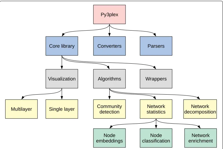
A high-level organization of the Py3plex library is shown in Fig.1. The library includes methods for parsing and converting graphs from and to various formats, while the core library includes three modules:
• The visualization moduleconsists of different subroutines used for network visualization of multilayer and single layer networks. Detailed description of the in-house developed visualization is given in “Py3plex multilayer network visualization” section.
• The wrappers moduleAs many procedures are given as standalone executables, Py3plex offers a set of wrapper subroutines, useful for calling external state-of-the-art algorithms, for example, highly optimized network embedding routines (Grover and
Fig. 1The Py3plex library architecture. The library is organized in hierarchical manner—a set of core data structures (blue) is used in algorithms for visualization and analysis of multilayer networks
Leskovec2016) as well as the InfoMap community detection algorithm (Rosvall et al.
2009). The methods offer easy access to multiplex community detection capabilities of Infomap, as well as community computation directly on the supra-adjacency matrix of a given network.
• The algorithms moduleincludes implementations of many commonly used algorithms, such as Louvain community detection (Blondel et al.2008), node ranking, network statistics, the recently introduced network topology enrichment (Škrlj et al.
2018), and network node classification and network embeddings.
All the modules are built in an extensible manner, allowing for new routines to be easily added. As Py3plex is built on top of the NetworkX (Hagberg et al.2008), network opera-tions can include any of the methods primarily designed for homogeneous networks. This functionality provides flexibility when implementing novel multilayer network analysis algorithms.
Key features
As Py3plex consists of multiple building blocks, we next describe key building blocks comprising the library. The set of data structures underlying all aforementioned modules offers intuitive access to manipulation, creation, and visualization of multilayer networks. Additionally, users of the library can use this core set of functionalities to implement their own algorithms. Other modules comprising Py3plex also build on top of the “multilayer network” object, a data structure we introduce for easier manipulation and consistency throughout the library.
outputs a visualization of choice. Detailed formulation of the supported visualizations is given in the following sections.
A substantial portion of Py3plex’s functionality is devoted to analysis of multilayer networks. Here, functionality such as network aggregation, centrality computation, and similar, offers straightforward analysis of the network’s properties. This part of the library also includes some of the state-of-the-art approaches for network decomposition and enrichments described in the following section.
Comparison of multilayer network libraries
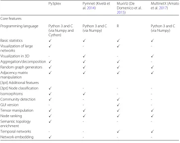
In this section, we compare the functionality of different multilayer network analysis and visualization libraries. Where relevant, we emphasize the novelties Py3plex offers and how they compare to existing alternatives4. Each library offers some functionality that is not available in other libraries, hence no library is exhaustive. We evaluate different aspects of functionality, ranging from their computational efficiency to the number of var-ious analysis functions provided. Table1presents the comparison of multilayer network analysis and visualization libraries, of which functionality is discussed in this section.
To ensure sufficient speed of execution, Pymnet (Kivelä et al.2014), Py3plex and Multi-netX (Amato et al.2017) include subroutine implementations in C (via Cython), but also Numpy (Walt et al.2011) and Scipy (Jones et al.2001) libraries for optimized lin-ear algebra-based computation. The R-based MuxViz (De Domenico et al.2015) uses the Octave library for efficient array-based operations.
Table 1Comparison of multilayer network analysis and visualization libraries
Py3plex Pymnet (Kivelä et
al.2014)
MuxViz (De Domenico et al. 2015)
MultinetX (Amato et al.2017)
Core features
Programming language Python 3 and C (via Numpy and Cython)
Python 3 and C (via Numpy)
R Python 3 and C
(via Numpy)
Basic statistics
Visualization of large
networks
-
-Visualization in 3D - -
Aggregation/decomposition
-Random graph generators
Adjacency matrix manipulation
[3pt] Additional features
[3pt] Node classification - -
-Isomorphisms -
-Community detection -
-GUI version - -
-Tensor manipulation
Node ranking
Semantic topology
enrichment
- -
-Temporal networks - -
Network embedding - -
In terms of visualization, all packages compared, include at least some form of net-work visualization. Apart from 2D layouts, The MuxViz and Pymnet libraries also support 3D layouts. As discussed in “Py3plex multilayer network visualization” section, Py3plex offers a new approach to multilayer network visualization, whereas Multi-netX, for example, is capable of displaying the supra-adjacency matrix (De Domenico et al. 2013) of the network. The multitude of different multilayer network visual-ization applications indicates that no single type of visualvisual-ization is optimal for a given task, as each visualization is optimal for a particular range of network size and density.
Apart from MultinetX, all other libraries compared above include different meth-ods for network aggregation and decomposition. A similar compendium of func-tionality is offered by Pymnet and MuxViz. All packages offer intuitive access to a network’s supra-adjacency matrix, and hence provide many opportunities for imple-mentation of computationally efficient multilayer network analysis algorithms. How-ever, Py3plex also leverages full functionality of the recently developed HINMINE (Kralj et al. 2018) methodology for heterogeneous network decomposition and net-work node classification. As standard aggregation schemes (De Domenico et al.2015) yield a homogeneous network, for example, by summing over edges in individual lay-ers, HINMINE-based aggregation is based on frequency of relation-annotated directed paths (of length two) between the target node type. Compared to standard aggrega-tion, HINMINE is thus suitable for situations where domain knowledge was used for annotating the network edges. Additionally, Py3plex also includes basic aggregation sub-routines, as well as supports classification using Personalized PageRank-based feature vectors is also supported (Kralj et al.2018). An interested reader can find the details in AppendixA.
All of the libraries listed above include methods for obtaining quick insights into a net-work’s structure. The Pymnet and Py3plex are currently the only libraries supporting different isomorphism algorithms for evaluating network similarity.
In terms of other functionalities, we observe the following. MuxViz also supports GUI-based analysis solutions, as well as API-GUI-based ones.Once installed, it can be executed locally within the browser as standalone software.
We observe Pymnet offers one of the most intuitive API interfaces for manipulation of tensor representations of multilayer networks, such as slicing, indexing etc. In com-parison, MultinetX and MuxViz offer similar functionality, whereas Py3plex operates on attribute-rich list-based representations of a network and is not necessarily suitable for all multilayer slicing tasks.
Aside from network analysis and visualization capabilities, Py3plex is the only library which also supports various forms of learning from multilayer networks. It provides the methodology for semantic enrichment of complex networks. The main objective in this emerging field is to associate previously known domain knowledge with topological structures of a network. For example, the functional characterization of a network’s com-munities can only be assessed using curated domain knowledge. We refer to the use of such knowledge to understand network-topological properties as network enrichment.
1 Partition detection. The network is partitioned into separate subnetworks, which commonly represent some form of functional similarity.
2 Enrichment. Individual communities are compared to the remainder of the network by using domain knowledge in the form of ontologies. Should a given ontology term (concept) be over- or under-represented in a considered
community, the community shall be considered enriched with respect to this term.
The end result of such analysis are thus community-term pairs, sorted by e.g., term sig-nificance. Currently, Py3plex is the only library that supports both rule-based enrichment as well as standard Fisher’s exact test-based enrichment, both introduced as part of the CBSSD methodology.
The current implementation of Py3plex contains wrapper routines for widely used net-work embedding algorithms, such as Node2vec and similar (Grover and Leskovec2016). Such functionality is currently not offered in any other libraries.
Overall, Py3plex offers novel algorithms for understanding network structure, an intu-itive interface for manipulation of multilayer networks as well as network decomposition and aggregation. However, the primary features of the current version of Py3plex are pri-marily network visualization and spatially efficient network manipulation (linear in terms of nodes and edges). This functionality offers additional state-of-the-art performance, not observed in the other libraries. Below, we first present the proposed network visualization (“Py3plex multilayer network visualization” section), followed by embedding-based node layout computation (“Embedding-based network layout” section), and finally on empirical evaluation of the proposed approaches on a set of artificial random multilayer networks, as well as real world biological and social networks (“Experimental evaluation” section).
Py3plex multilayer network visualization
One of the key contributions of this paper is a novel method for visualization of multi-layer networks. In this section, we showcase the proposed visualization method and its implementation. Next, we evaluate the method’s performance on a series of random net-works, where we subsequently compare the results with Pymnet’s network visualization capabilities.
Visualization methodology and implementation
The proposed set of visualization techniques aims to address the issue of visualizing mul-tilayer networks. The implementation of the presented layout algorithm operates in three main steps described below.
algorithm (based on Barnes-Hutn-body minimization), which was transpiled from Python to C, is used as the default option during visualization (Jacomy et al.2014). Throughout the work, we refer to such layouts as spring layout plots.
Multilayer network drawing. In the second step, nodes are drawn along a diagonal line based on their type (i.e. layer they belong to). This is achieved by calculating the actual coordinates of each point by separating each consecutive layer from the pre-ceding layer by exactly a single coordinate unit on both axes. The result is that, for a node in thei-th layer, where we calculated coordinates(x,y)in step 1, we now update the coordinates to(x+i,y+i). As nodes in different layers are now separated by at least one coordinate unit, each subnetwork corresponding to different node type is drawn in a separate region with no overlap between different layers. Each layer includes a network with its own local organization, independent of the inter-layer connections.
Inter-layer edge drawing. The final step involves drawing of inter-layer edges, which are represented as arces connecting different nodes. One of the main problems we faced during the implementation of this step was edge positioning and parameteri-zation, as there are many different ways of drawing an arc between two nodes. We considered three possible scenarios in terms of inter-layer edge drawing:
1 The edges are only on the upper part of the layer diagonal; 2 The edges are only on the bottom part of the layer diagonal; 3 The edges are on both sides of the diagonal projection.
An inter-layer edge between nodesn1andn2of the network (represented by points
(x1,y1)and(x2,y2), respectively) is drawn as follows. First, an artificially introduced point
(x3,y3)is calculated by taking the midpoint between(x1,y1)and(x2,y2)and scaling its
ycoordinate by a factor ofτ (a parameter of the method). Scaling theycoordinate by a fixed amount (τ) instead of shifting it ensures that each edge is, in effect, shifted up by a different value, allowing all edges to be visible in the final image. Changing the value of parameterτ offers simple manipulation of inter-layer edges as follows:
1 whenτ >1, the arc will be located above the diagonal;
2 whenτ =1, the arc will be a line between the two nodes (a third point onf(x)); 3 whenτ <1, the arc will be located below the diagonal.
Oncen1,n2andn3are obtained, pointsn1andn2are connected by a parabolic arc that
passes through all three points. Even though the current implementation constructs inter-layer edges using interpolation over three points, Py3plex supports adding an arbitrary number of intermediary points, in which case cubic arc interpolation is used to produce the line between n1andn2. In our experiments, however, we show that even a single
intermediary point allows for clear visualization.
We further propose a heuristic for automatically determining an arc’s position, i.e. whether an arc should be located above or below the diagonal. We achieve this as follows. Given n1 and n2 as defined in the previous paragraph, the arc is located
above the diagonal if and only if int(n3) > n3, where int(n3) represents the
inte-ger representation of the coordinates of n3. Integer-based rounding works, as layers
appear incomprehensible, natural logarithms are applied to node representations— filled circles based on individual node degrees—which simplifies visualization of denser networks.
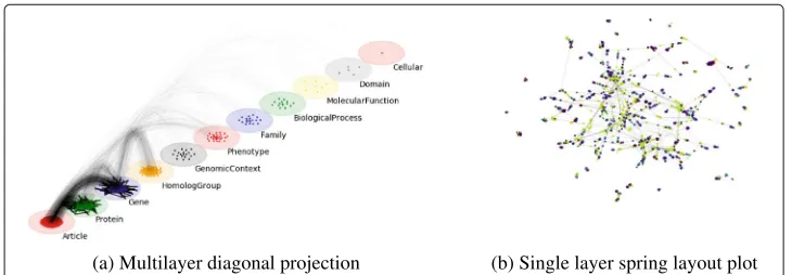
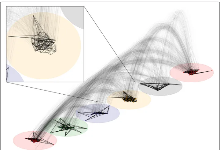
Py3plex can easily visualize more than ten layers with tens of thousands of nodes. Com-pared to existing solutions, diagonal projection of multiple layers enables visualization using standard layout algorithms, with additional specification of inter-layer edges. An example visualization using the presented Py3plex library is shown in Fig. 2, with an alternative visualization using a single layer force-directed layout of the whole network is included for comparison.
Strengths and potential drawbacks
In this section, we discuss the strengths and weaknesses of the proposed visualization. We begin by describing the strengths and continue with the discussion of the cognitive load and other potential drawbacks.
Strengths
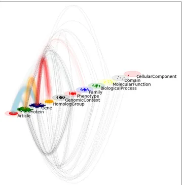
Many aspects of the visualization presented in this paper can be customized to empha-size either the node or layer properties. For example, in Fig.3we colored differently the inter-layer edges corresponding to specific relations. Additionally, such edges can be plot-ted either on the upper or the lower side of the diagonal containing networks, making it possible for the user to emphasize only the selected inter-layer edges. The height, types of lines, colors and transparency can be fine-tuned to the user’s preferences. The colors of intra-layer edges and nodes can also be customized—for example, special nodes or sets of nodes can be colored to emphasize the intra-layer structure.
Potential drawbacks
In this section, we also discuss some of the drawbacks the presented approach intro-duces, especially when considering larger networks. One of the main problems with such complex visualizations is the amount of overlapping edges, which was shown to be prob-lematic for the user experience by Purchase (1997). We split the following discussion into two main parts: intra-layer overdrawing and inter-layer overdrawing.
Fig. 3A customized Py3plex visualization. Here, the blue inter-layer edges correspond torefers torelation, orange ones tocodes forand red tobelongs torelation
Intra-layer edge overdrawing. Non-planar, real-world networks are impossible to draw without some edge overlap. The problem with drawing networks within layers is thus inherent to all other libraries which visualize such network. Py3plex tackles this issue by enhancing transparency of edges based on density, edge threshold-ing, as well as controlling edge widths. Further, node sizes also take up substantial amounts of layout space, thus need to be adapted accordingly. Even though the space in which individual intra-layer networks are drawn is smaller than the whole canvas, the Force Atlas 2 algorithm which is used for intra-layer layout computation, dis-perses the nodes based on their connectivity patterns. This way, it partially separates the densely connected clusters (some arc overlap is reduced this way). To preserve topological properties of intra-layer networks, some overlap (e.g., within functional clusters) is inevitable.
layers on the upper and the lower part of the main diagonal, some of the edge over-lap can be reduced by redistributing the edges accordingly across the empty regions of the canvas. Such positioning can be automaticaly determined by Py3plex. Next, heights of individual arcs can be manually configured, enabling definition of cus-tom, less overlapping groups of arcs. While presented solutions do not entirely solve the problem, we believe that for non-planar graphs (especially in 2D), if the user knows what aspect to emphasize, the proposed solution can provide sensible visual-izations. While separating the layers may incur more overall edge overdrawing, we believe that this cost is outweighed by the benefits (i.e. added visual clarity offered by visually separated layers) of our visualization.
Finally, we discuss how intra- as well as inter-layer edges contribute to understanding of the plots. Should the number of inter-layer edges increase in layers that are very close together, such setting is prone to cognitive overload and can be addressed by specifying a different layer order. Very sparse networks with many layers are also harder to visualize using the presented visualization, as with many layers, information regarding connectivity can become harder to comprehend—the inter-layer edges can span across larger regions of canvas and are harder to follow.
Cognitive load
In this section we discuss the potential implications of the presented methodology with respect to cognitive load, as this aspect of visualization can be critical in determining the usability of a given visualization method. This section follows guidelines from Huang et al. (2009), who investigated how complex networks remain understandable to a non-expert human observer. Via a variety of cognitive tasks (such as triangle counting), Huang et al. showed that networks with only tens of nodes and hundreds of edges can already pose a problem when it comes to their interpretation and understanding. While the work by Huang et al. is not focused on multilayer networks, visualization properties they recognize as relevant are also applicable when visualizing multilayer networks.
Huang et al. (2009) identify several key factors of cognitive load presented by a given network visualization. The factors that are most relevant for the following discussion regarding cognitive load of Py3plex plots are the following:
Domain complexity. Not all domains are equally complex. Huang et al. point out that visualizations of biological networks should differ from the ones used for displaying social networks. Py3plex is adapted in line with these findings. The layer-level diagonal visualization introduced in this work offers intuitive segmentation of e.g., biological information (e.g., DNA, RNA, protein etc.); however, such levels are not necessarily present in social networks. In order to address this issue, Py3plex offers functionality to aggregate layers, which can be adapted to specific use-cases.
Visual complexity. Visualizations can have varying degrees of complexity. Here, aspects such as edge or node overlaps and the number of different elements visu-alized need to be considered. The complexity of the visualizations obtained using Py3plex can be high, as it displays multiple layers along with inter- and intra-layer edges. We refer the reader to “Potential drawbacks” section for detailed discussion of the visualization aspects which influence the final output the most.
Interactivity
Because one of the output options supported by Py3plex is a Matplotlib canvas (Hunter
2007), the resulting visualizations can easily be:
• Zoomed-into. A square region of the visualization is selected and zoomed-into. This functionality offers e.g., a way to emphasize only certain layers of interest.
• Stretched. The interactive viewer offers simple functionality for adapting the shape of the resulting visualization, offering fine-tuning with respect to e.g., overlapping text.
• Animated. Matplotlib offers animation functionality, making possible the construction of e.g., dynamic visualizations, consisting of multiple (e.g.,
time-dependent) frames. An example of such an animation is available online in .gif format5.
Embedding-based network layout
Visualization of large networks commonly results in long computation times and incom-prehensible layouts. Recent advancements in the field of machine learning on graphs can be leveraged to facilitate the process of network visualization. Even though embedding-based data visualization is becoming commonplace in contemporary machine learning, such techniques span back to Harel and Koren (2002), who initially investigated how network embeddings can be used for visualization. They use principal component anal-ysis (PCA) as the main embedding mechanism. Even though PCA can offer valuable insights when projecting the data into orthogonal space of lower dimension, it does not necessarily maintain all network-topological properties which represent key parts of the considered network. The initially considered network embedding (PCA) does not take into account higher-order node neighborhoods, missing out on e.g., densely connected parts of networks that can only be accessible when considering longer random walks.
This section is structured as follows. First, we describe the role of network embed-ding algorithms in a standard machine learning setting. Next, we show how methods for non-linear dimensionality reduction can be combined with scalable node embeddings for network layout construction. Finally, we present a simple benchmark of the presented layout algorithm compared with a generic, force-directed layout.
Network embedding
Recent advancements in learning from complex networks commonly consist of two main steps: network embedding and learning. Recent approaches for embedding construction include DeepWalk (Perozzi et al.2014), Node2vec (Grover and Leskovec2016), Struc2vec (Ribeiro et al.2017), and similar approaches, all of which attempt to capture node infor-mation and encode it in the form ofd-dimensional vectors. In this work we are interested
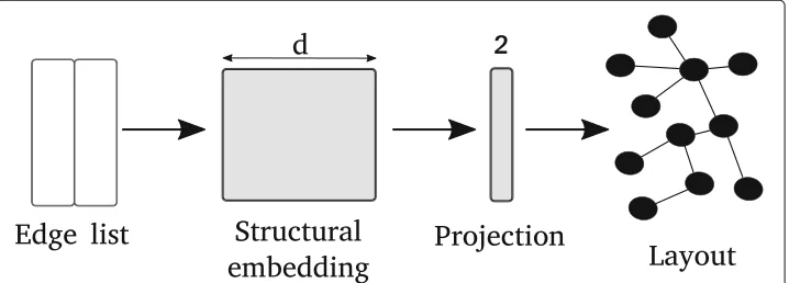
in the embedding phase of the these algorithms, as well as the use of resulting node embeddings as the first step in the presented layout calculation algorithm. The feature matrix (table) can be used with less additional preprocessing compared to sophisticated relational nature of a graph. The presented visualization approach first constructs such an embedding, and subsequently projects it to a two-dimensional vector space; this space of(x,y)pairs represents initial node coordinates. Schematic representation of this idea is shown in Fig.4.
We next describe some of the key steps of node2vec, as recently given in (Kralj et al.
2019). We believe understanding of how node2vec operates shall offer the reader intu-ition as to why use the selected embedding method as a building block of the proposed visualization.
Network embedding using node2vec
A recently developed approach to vectorizing network nodes is the node2vec algorithm (Grover and Leskovec2016), which uses the random walks to calculate features that express similarities between pairs of nodes.
The node2vec algorithm takes as input a network ofnnodes, represented as a graph
G=(V,E)whereV is the set of network nodes andEis the set of connections, or edges, in the network. The algorithm returns a matrixf ∈R|V|×dwith a pre-defined number of columnsd. Matrixf is interpreted as a collection ofd-dimensional feature vectors with the i-th row of the matrix corresponding to the feature vector of thei-th node in the network. We writef(u)to mean the row of matrixf, corresponding to nodeu. The goal of the algorithm is to construct feature vectorsf(u)in such a way that the feature vectors of all nodes that share a certain neighborhood will be similar. Matrixf is calculated as follows:
E(G)=arg Max
f∈R|V|×d
u∈V ⎛ ⎝−log
v∈V
ef(u)·f(v)
+
ni∈NS(u)
f(ni)·f(u) ⎞
⎠ (1)
whereN(u)denotes the network neighborhood of nodeugiven asampling strategy, and
Ethe embedding constructor (node2vec in this case). In the above expression the inner sum calculates the similarities between a node and all nodes in its neighborhood. This
sum is large if the feature vectors of nodes in the same neighborhood are collinear, how-ever it also increases if feature vectors of nodes have a large norm. The first value of each summand decreases when the norms of feature vectors increase, thereby penalizing collections of feature vectors with large norms.
Expression (1) has a probabilistic interpretation which models a process of randomly selecting nodes from the network. The probabilityP(n|u) of noden following nodeu
in the selection process is proportional toef(n)·f(u). Assuming that selecting one node is
independent from selecting any other node, we can calculate the probability of selecting all nodes from a given setAasP(A|u)= n∈AP(n|u), and Eq.1can then be rewritten as follows:
E(G)=arg Max
f∈R|V|×d
u∈V
logP(NS(u)|f(u))
. (2)
TermNS(u)in Eqs. (1) and (2) denotes the neighborhood ofugiven a sampling strategy
Sand is calculated by simulating a random walker traversing the network starting at node
u. The transition probabilities for traversing from noden1 to noden2depends on the
noden0the walker visited before noden1, making the process of traversing the network
a second order random walk. The unnormalized transition probabilities are set using two parameters,pandq, and are equal to:
P(n2|previous step moved from noden0ton1)= ⎧ ⎪ ⎨ ⎪ ⎩ 1
p ifn2=n0
1 ifn2can be reached fromn1 1
q otherwise
.
Parameterspandqare referred to as thereturnparameter and thein-out parameter, respectively. A low value of the return parameterpmeans that the random walker is more likely to backtrack its steps, meaning the random walk will be closer to a breadth first search. On the other hand, a low value of the parameterqencourages the walker to move away from the starting node and the random walk resembles a depth first search of the network. To calculate the maximizing vectorf, a set of random walks of limited size is simulated starting from each node in the network to generate several samples of the set
NS(u).
The function maximizing expression (1) is calculated using stochastic gradient descent. The value of (1) is estimated at each generated sampling of the neighborhoodsNS(u)for
all nodes in the network to discover the vectorf that maximizes the expression for the simulated neighborhood set.
Extensions to multilayer networks
Reducing embedding dimensionality using t-SNE
Note that even though the nodes of a network can be embedded in 2 dimensional space directly, the obtained representations are normally not representative of the network’s structure. IfE(G)represents the network embedding function, we introduce an additional operation,P(E(G)), i.e. a projection of the obtained network embedding (see previous section) to a 2-dimensional, real-valued vector space. Embedding-based graph drawing was previously proven to scale to very large networks (Hachul and Jünger2006), thus we believe similar ideas implemented with more recent approaches could offer similarly good performance on large multilayer networks with many layers.
In the experiments shown in the following sections, we use t-SNE projections (Maaten and Hinton2008) for obtaining the final set of node coordinates. The t-SNE algorithm taks as input a set of high dimensional vectors and projects them to a low-dimensional vector space while maintaining (as much as possible) the similarities between the vec-tors. For use in data visualization, the low-dimensional space has dimension 2 or 3. The algorithm works in two steps.
1 Similarities between pairs of input vectors (in our case, thed -dimensional node embeddings) are calculated.
2 Low-dimensional vectors are calculated such that the vector-pair-similarities of the low dimensional vectors re-create the original similarities as closely as possible.
Similarities between input vectors{x1,. . .,xn} are modeled as follows. Letxi andxj
denote two points in the inputd-dimensional embedding. The similarity between data pointxjandxiis modeled as the probability thatxiwould pickxjas its neighbor if
neigh-bors were picked in proportion to their probability density under a Gaussian centered at
xiand is calculated as follows:
pij=
e
−||xi−xj||2/2σi2
g=he
−||xg−xh||2/2σi2
,
whereσiis the variance of the Gaussian, centered on data pointxi. In t-SNE,σiis
deter-mined so that theperplexityof the Gaussian equals a fixed value, specified by the user. The desired perplexity parameter can be interpreted as the number of neighbors of each data point. Frompi|j, the joint probabilitypijis calculated aspij= pj|i2n+pi|j.
In finding the low-dimensional representation{y1,. . .,yn}, t-SNE models similarities
between pairs of representation vectors using the Cauchy distribution, calculated as follows:
qij=
1+ ||yi−yj||2−1
g=h
1+ ||yg−yh||2 −1.
Using this model, t-SNE uses stochastic gradient descend to minimize the Kullback-Leibler divergence (Kullback and Kullback-Leibler1951) between the original probabilitiespijand
the new probabilitiesqij. We refer the interested reader to the original paper (Maaten and
Hinton2008) for technical details of this optimization.
Final formulation
two fundamentally different mappings. First,Eattempts to capture a given node’s neigh-bourhood information, whilstPattempts to construct a low-dimensional embedding by preserving the input’s dimension (distances between input feature vectors).
The mappingsEandP are applied sequentially to obtain coordinate tuplestxy ∈ R2,
wheretxy can already serve as the coordinates for plotting individual nodes, or can be
used as the initialization of the force-directed layout. The presented algorithm can thus be described in three simple steps:
1 Network embedding intod -dimensional vector space.
2 Projection ofd -dimensional embeddings into two dimensions. 3 (Optional) few iterations of distance minimization.
For the experimental evaluation discussed in the next section we used node2vec for the network embedding part, and t-SNE for projections. Note that the idea discussed in this section is both embedding, as well as projection-agnostic—arbitrary embedding algo-rithm’s output can be projected to two dimensions using an arbitrary projection method. We recognize as relevant related work the body of literature focusing on node embedding learning, summarized in (Goyal and Ferrara2018), a survey in which node2vec proved to be one of the best performing algorithms. Similarly, the recently introduced Embedding Projector (Smilkov et al.2016) offers visualization of embeddings projected via PCA or other non-linear projections.
Experimental evaluation
In the following sections, we discuss the performance of Py3plex with respect to visual-ization, as well as analysis tasks. We begin by comparing the proposed embedding-based layout to some of the contemporary layout algorithms. Next, we demonstrate the scal-ability of the library and conclude with an analysis of a dynamic multiplex social network.
Experiment one: benchmark of layout computation time
We next present a simple benchmark, where we tested the speed of the presented method in comparison with the Force Atlas 2 algorithm (FA2) (which uses Barnes-Hut approxi-mation for the n-body problem for faster minimization). We used the FA2 algorithm as it is widely used in software such as Gephi (Bastian et al.2009), representing a relevant baseline for this task.
and 400,000 edges. We computed layouts for each network five times, and averaged the computation times.
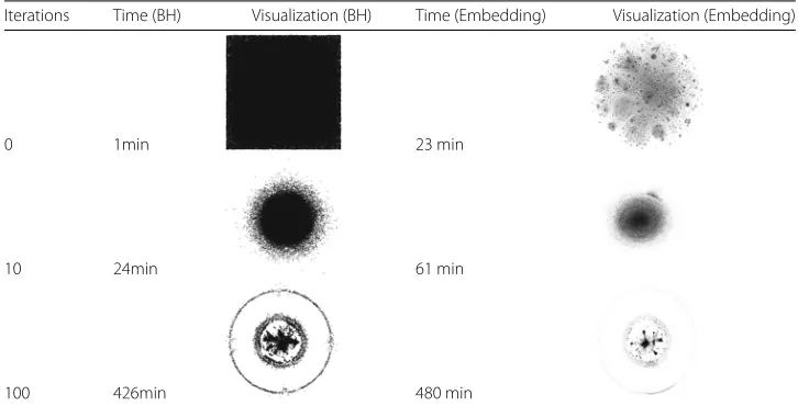
The obtained benchmark times along with computed layouts are summarized in Table2. It can be observed that the embedding based layout looks notably different to any of the force-directed ones. After many rounds of minimization, the embedding based lay-out starts to resemble the force-directed one. We believe this experiment demonstrates the power of using network embeddings for qualitative analysis. We additionally dis-cuss the obtained results in “Conclusions and further work” section. We continue with a benchmark study, where we compare the visualization time of Py3plex, compared with Pymnet, an alternative Python based library for visualization of such networks.
Experiment two: overall performance
In this section we first present the result of comparing visualization times of Py3plex and Pymnet libraries. Next we discuss a practical case study where we visualize a multiplex dynamic social network. Multiplex networks are comprised of the same set of nodes pro-jected across layers. Here, no physical inter-layer edges are commonly present, as they correspond tois arelation.
We present the results for the times needed to obtain a visualization of networks of different complexities; here, we compare Py3plex to Pymnet library. Even though Pym-net does not support the diagonal projection and Py3plex does not support the default 3D linear projections, both methods are useful for visualization of different aspects of multilayer networks.
The main aim of this section is to demonstrate that Py3plex offers better support for visualization of larger networks.
The experimental setting for this task was designed as follows. Random multilayer Erd˝os-Rényi (ER) networks were generated using the Pymnet (Kivelä et al.2014) library. We used this network model purely for its simplicity and control over the node and edge space. While ER networks do not exhibit such real-world properties as, for example, Stochastic Block Models (Holland et al.1983), we believe the larger ER networks con-sidered exhibit enough complexity for comparisons to be meaningful for the concon-sidered
Table 2Comparison of force directed layout with the presented embedding based layout
Iterations Time (BH) Visualization (BH) Time (Embedding) Visualization (Embedding)
0 1min 23 min
10 24min 61 min
100 426min 480 min
comparisons — in this section, we are only interested in comparing the computation time needed to visualize the networks. As the computation and visualization times are mostly dependent on the numbers of nodes and edges, if Py3plex outperforms Pymnet on these networks, we also expect it to outperform Pymnet on other networks of comparable size. Such random networks are parameterized using parameterNcorresponding to the total number of nodes, parameterLcorresponding to the number of layers, and parameterp
corresponding to the re-wiring probability. We generated the networks in the following parameter ranges:
p∈ {0.05, 0.1, 0.2, 0.3},
N∈ {5, 10, 20, 50, 80, 100},
L∈ {1, 2, 3, 4, 5, 6, 7, 8, 9, 10}.
Once generated, the time needed for visualization was recorded. We compared visu-alization times of Pymnet and Py3plex, as the remaining Python-based alternative, MultinetX, does not support drawing of coupled edges.
We show the final results of our experiment in the form of box plots, where|N| or
|E|is plotted on thex-axis and the time needed is plotted on they-axis (Figs.5and6). Networks with more than 100 nodes were not considered for this benchmark, as it took Pymnet more than two hours for visualization. Nonetheless, Py3plex was able to visu-alize a network with|N| = 4,000 and|E| = 18,600 under two hours, even though the obtained network is not necessarily useful for visualization purposes. The machine used for benchmark testing was an off-the-shelf Lenovo y510p laptop.
Visualization of dynamic multiplex networks
Real-world multilayer or multiplex networks are commonly subject to either edge or node dynamics; for example, friendships form over time, or biological phenotypes emerge and disappear (Secrier et al.2012). Here, the number of e.g., edges can be subject to notable
Fig. 6Time consumed to produced the visualization. Time with respect to the number of nodes is shown in (a), and time with respect to the number of edges in (b)
change, hence the temporal component of a given network can not be neglected. In this section we showcase some of Py3plex’s rather simple extensions to dynamic networks. A natural representation for a dynamic network is some form of video output, where indi-vidual e.g., time windows or slices are used as frames. We present Py3plex’s functionality for production of such frames.
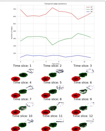
We consider a dynamic multiplex social network initially introduced in Omodei et al. (2015). Here, the same set of users is observed in terms of retweets, mentions and com-ments. We represented the network by considering eachtype of interactionas a separate layer, as the users remain the same. The network consists of 392,000 users, we consider more than 100,000 time points, each representing an event (edge) between the users. The edges represent either retweets, mentions or comments.
Visualization preparation
As the users in separate layers are the same, we do not plot any inter-layer edges, as in the presented visualization they do not contain any added value and only result in cognitive overload. Next, we compute layouts for individual nodes as follows. We first create a sim-pler, homogeneous network consisting of all users. There, we compute the layout for each node. We use the same layout for each layer, hence, for example, a node’s position in e.g.,
theretweetlayer directly corresponds to the one in e.g.,mentionslayer.
We take into account the network dynamics (temporal links) by considering time slices of size 12,000. Although there exist more intricate methods for taking into account the temporal information, we believe the presented visualization serves the demonstration purpose, as it can easily be extended to e.g., a moving window scenario. For clarity, we do not display isolated nodes.
Visualization result
The resulting visualization is shown in Fig. 7. The considered time granularity (1000 points) yields re-tweet and mention networks (red and green) with constant activity. The response network (blue) is subject to the highest variability in terms of link quantity. At e.g., slices 3, 10 and 22 the network is subject to high activity — we believe this indicates the spread of viral news. Other slices, such as for example 8 and 9 indicate there are also periods, when only a few mentions appear.
Conclusions and further work
We have developed and implemented Py3plex, a network analysis and visualiza-tion library focused on multilayer networks. In addivisualiza-tion to most of the funcvisualiza-tional- functional-ity offered by other state-of-the-art libraries, Py3plex introduces a novel visualiza-tion, suitable for larger multilayer networks, as to our knowledge, there currently do not exist any methods that can visualize networks composed of thousands of nodes along with their intra- as well as inter-layer organization. Py3plex is suitable for the development of algorithms, as it offers fast lookup and indexing routines, which scale to networks consisting of multiple layers with hundreds of thousands of edges.
One of the new concepts introduced in this paper is a novel multilayer net-work visualization layout. Py3plex plots intra-layer connections separately to the inter-layer ones, yielding more comprehensive visualizations. We belive the presented diagonal projection could also be extended into an additional dimension (orthogo-nal), hence offering more efficient space consumption. The presented library cur-rently only includes primitive tools for animating multilayer networks—here, the temporal component is split into small slices, which are animated (network snap-shots are merged into a single animation). We believe this aspect of Py3plex could be further improved, as many real-world multilayer networks also have a dynamic component.
Another novelty of this work is embedding based visualization. We believe the exper-iments conducted serve as a proof of concept, yet we believe many other embedding algorithms could also be used to improve the layout’s quality. Furthermore, the recently introduced UMAP algorithm (McInnes et al. 2018) could also be used instead of t-SNE, making the layout computation even more scalable. We believe this embedding could be especially useful in situations where larger networks with distinct topolog-ical structure are considered. Even though we demonstrated the embedding based layout on a biological network we believe it could serve as a viable visualization alter-native to visualize other types of networks, such as for example the transportation vnetworks.
In this work, we compared the visualization capabilities of Py3plex to these of the Pymnet library. Even though we demonstrated that Py3plex layout scales bet-ter, Pymnet’s 3D visualization is better suited for small demonstrative purposes, where the key idea of a studied system needs to be conveyed as clearly as possi-ble. We believe that the two libraries are in this sense complementary, as we found Py3plex to be the preferrable tool used for visualization of actual, larger multilayer networks.
In terms of scalability, we attempted to re-implement some of the common bot-tlenecks, such as the layout computation, aggregation, and indexing using effi-cient vectorized operations. However, we have yet to improve the traversal algo-rithms, as they are not the key focus of this work. We will re-implement random graph generation and crawling first in C, and eventually on GPUs for maximum performance.
entanglement (Renoust et al.2014), which was constructed using only the data structures offered by Py3plex. By offering fast prototyping, this library can serve to exchange the ideas related to multilayer network analysis.
One of the main drawbacks of Py3plex visualizations is the cognitive load. While the user can currently observe high-level organization of a multilayer network, it can be hard to interpret the structure of individual layers and their contributions to the structure of the whole network. Even though Py3plex can plot directly to an interactive canvas, we believe this issue represents an interesting research direction and will be addressed in follow up work.
As the Py3plex analysis suite is by no means exhaustive, further work includes the implementation of network dynamics analysis methods as well as the more effi-cient, GPU-based random samplers. Py3plex aims to bridge the gap between machine learning approaches and complex networks, and it does not yet include extensive tensor manipulation, unfolding, and construction routines offered in the Pymnet library.
Appendix A: Network decomposition functions
In this section, we give an overview of the heterogeneous network decomposition functions introduced in HINMINE (Kralj et al.2018), supported by Py3plex.
Given a heuristic functionf, a weightwof an edge between the two nodesuandvis computed as follows:
Let Bdenote the set of all nodes of the base type. We use the following notations:
f(t,d)denotes the number of times a termtappears in the documentdandDdenotes the corpus (a set of documents). We assume that the documents in the set are labeled, each document belonging to a class cfrom a set of all classesC. We use the notation
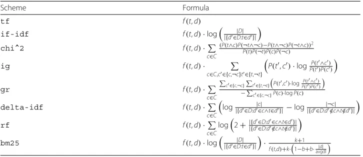
t ∈ dto describe that a termtappears in document d. Where used, the termP(t)is the probability that a randomly selected document contains the termt, andP(c)is the probability that a randomly selected document belongs to classc. We use|d|to denote the length (in words) of a document, and avgdl denotes the average document length in the corpus. All weight functions (heuristics) supported by Py3plex are summarized in Table3.
Table 3Term weighing schemes, taken from (Kralj et al.2018), tested for decomposition of heterogeneous networks and their corresponding formulas
Scheme Formula
tf f(t,d)
if-idf f(t,d)·log|{d∈|DD:t|∈d}|
chi^2 f(t,d)·
c∈C
(P(t∧c)P(¬t∧¬c)−P(t∧¬c)P(¬t∧c))2 P(t)P(¬t)P(c)P(¬c)
ig f(t,d)·
c∈C,c∈{c,¬c}t∈{t,¬t}
P(t,c)·logPP((tt)∧P(cc))
gr f(t,d)·
c∈C
c∈{c,¬c}t∈{t,¬t}
P(t,c)·logPP((tt∧)P(cc))
−c∈{c,¬c}P(c)·logP(c)
delta-idf f(t,d)·
c∈C
log|{d∈D:d|c∈|c∧t∈d}|−log|{d∈D:d|¬∈/cc|∧t∈/d}|
rf f(t,d)·
c∈C
log2+|{|{dd∈∈DD::dd∈∈/cc∧∧tt∈∈/dd}|}|
bm25 f(t,d)·log|{d∈|DD:t|∈d}|
· k+1 f(t,d)+k·1−b+b·|d|
Acknowledgements
We would like to thank to Lucija Luetiˇc for proofreading the manuscript, which notably improved the work’s quality. The work of the first author was funded by the Slovenian Research Agency through a young researcher grant. The work of other authors was supported by the Slovenian Research Agency (ARRS) core research programmeKnowledge
Technologies(P2-0103) and ARRS funded research projectSemantic Data Mining for Linked Open Data(financed under the ERC Complementary Scheme, N2-0078). The work was supported also by European Union’s Horizon 2020 research and innovation programme under grant agreement No 825153, project EMBEDDIA (Cross-Lingual Embeddings for Less-Represented Languages in European News Media).
Authors’ contributions
The authors’ contributions are as follows. BŠ and JK implemented the library and conducted the experiments. BŠ, JK and NL designed the experiments and conducted theoretical overviews and analysis. All authors read and approved the final manuscript.
Availability of data and materials
The Py3plex library as well as the datasets used in this paper are freely accessible at web sitehttps://github.com/SkBlaz/ Py3plex, where many working examples of the Py3plex functionality are also offered.
Competing interests
The authors declare that they have no competing interests.
Received: 9 March 2019 Accepted: 30 August 2019
References
Amato R, Kouvaris NE, San Miguel M, Díaz-Guilera A (2017) Opinion competition dynamics on multiplex networks. New J Phys 19(12)
Auber D, Archambault D, Bourqui R, Delest M, Dubois J, Lambert A, Mary P, Mathiaut M, Mélançon G, Pinaud B, et al. (2017) TULIP 5. Springer
Auber D (2004). In: Jünger M, Mutzel P. (eds). Tulip — A Huge Graph Visualization Framework. Springer, Berlin. pp 105–126 Bastian M, Heymann S, Jacomy M (2009) Gephi: an open source software for exploring and manipulating networks. In:
Third International AAAI Conference on Weblogs and Social Media
Batagelj V, Mrvar A (2001) Pajek—analysis and visualization of large networks. In: International Symposium on Graph Drawing. Springer. pp 477–478
Blondel VD, Guillaume J-L, Lambiotte R, Lefebvre E (2008) Fast unfolding of communities in large networks. J Stat Mech Theory Exp 2008(10):10008
Boccaletti S, Bianconi G, Criado R, del Genio CI, Gómez-Gardeñes J, Romance M, Sendiña-Nadal I, Wang Z, Zanin M (2014) The structure and dynamics of multilayer networks. Phys Rep 544(1):1–122
De Domenico M, Nicosia V, Arenas A, Latora V (2015) Structural reducibility of multilayer networks. Nat Commun 6:6864 De Domenico M, Porter MA, Arenas A (2015) MuxViz: A tool for multilayer analysis and visualization of networks. J
Complex Netw 3(2):159–176
De Domenico M, Solé-Ribalta A, Cozzo E, Kivelä M, Moreno Y, Porter MA, Gómez S, Arenas A (2013) Mathematical formulation of multilayer networks. Phys Rev X 3(4).https://doi.org/10.1103/physrevx.3.041022
Goyal P, Ferrara E (2018) Graph embedding techniques, applications, and performance: A survey. Knowl-Based Syst 151:78–94
Grover A, Leskovec J (2016) Node2vec: Scalable feature learning for networks. In: Proceedings of the 22Nd ACM SIGKDD International Conference on Knowledge Discovery and Data Mining, KDD ’16. ACM, New York. pp 855–864 Hachul S, Jünger M (2006) An experimental comparison of fast algorithms for drawing general large graphs. In: Healy P,
Nikolov NS (eds). Graph Drawing. Springer, Berlin, Heidelberg. pp 235–250
Hagberg A, Swart P, S Chult D (2008) Exploring network structure, dynamics, and function using NetworkX. In: Proceedings of the 7th Python in Science Conference (SciPy)
Harel D, Koren Y (2002) Graph drawing by high-dimensional embedding. In: International Symposium on Graph Drawing. Springer. pp 207–219
Holland PW, Laskey KB, Leinhardt S (1983) Stochastic blockmodels: First steps. Soc Networks 5(2):109–137
Huang W, Eades P, Hong S-H (2009) Measuring effectiveness of graph visualizations: A cognitive load perspective. Inf Vis 8(3):139–152
Hunter JD (2007) Matplotlib: A 2d graphics environment. Comput Sci Eng 9(3):90
Jacomy M, Venturini T, Heymann S, Bastian M (2014) ForceAtlas2, A continuous graph algorithm for handy network visualization designed for the Gephi software. PloS ONE 9(6):98679
Jones E, Oliphant T, Peterson P, et al (2001) SciPy: Open source scientific tools for Python
Kivelä M, Arenas A, Barthelemy M, Gleeson JP, Moreno Y, Porter MA (2014) Multilayer networks. J Complex Netw 2(3):203–271
Kullback S, Leibler RA (1951) On information and sufficiency. Ann Math Stat 22(1):79–86
Kralj J, Robnik-Šikonja M, Lavraˇc N (2018) HINMINE: Heterogeneous Information Network Mining with Information Retrieval Heuristics. J Intell Inf Syst 50(1):29–61
Kralj J, Robnik-Sikonja M, Lavrac N (2019) Netsdm: Semantic data mining with network analysis. J Mach Learn Res 20(32):1–50
Leskovec J, Sosiˇc R (2016) Snap: A general-purpose network analysis and graph-mining library. ACM Trans Intell Syst Technol 8(1):1–1120
McGee F, Ghoniem M, Melançon G, Otjacques B, Pinaud B (2019) The state of the art in multilayer network visualization. Comput Graph Forum 0(0).https://doi.org/10.1111/cgf.13610
McInnes L, Healy J, Melville J (2018) Umap: Uniform manifold approximation and projection for dimension reduction. arXiv preprint arXiv:1802.03426
Nepusz G, Csárdi G (2006) The igraph software package for complex network research. Complex Syst 1695(5):1–9 Omodei E, De Domenico MD, Arenas A (2015) Characterizing interactions in online social networks during exceptional
events. Front Phys 3:59
Orchard S, Ammari M, Aranda B, Breuza L, Briganti L, Broackes-Carter F, Campbell NH, Chavali G, Chen C, Del-Toro N, et al (2013) The mintact project—intact as a common curation platform for 11 molecular interaction databases. Nucleic Acids Res 42(D1):358–363
Pavlopoulos GA, O’Donoghue SI, Satagopam VP, Soldatos TG, Pafilis E, Schneider R (2008) Arena3d: visualization of biological networks in 3d. BMC Syst Biol 2(1):104
Perozzi B, Al-Rfou R, Skiena S (2014) Deepwalk: Online learning of social representations. In: Proceedings of the 20th ACM SIGKDD International Conference on Knowledge Discovery and Data Mining, KDD ’14. ACM, New York. pp 701–710 Purchase H (1997) Which aesthetic has the greatest effect on human understanding? In: International Symposium on
Graph Drawing. Springer. pp 248–261
Renoust B, Melançon G, Viaud M-L (2014). In: Missaoui R, Sarr I (eds). Entanglement in Multiplex Networks: Understanding Group Cohesion in Homophily Networks. Springer, Cham. pp 89–117
Ribeiro LFR, Saverese PHP, Figueiredo DR (2017) Struc2vec: Learning node representations from structural identity. In: Proceedings of the 23rd ACM SIGKDD International Conference on Knowledge Discovery and Data Mining, KDD ’17. ACM, New York. pp 385–394
Rosvall M, Axelsson D, Bergstrom CT (2009) The map equation. Eur Phys J Spec Top 178(1):13–23
Secrier M, Pavlopoulos GA, Aerts J, Schneider R (2012) Arena3d: visualizing time-driven phenotypic differences in biological systems. BMC Bioinformatics 13(1):45
Shannon P (2003) Cytoscape: A software environment for integrated models of biomolecular interaction networks. Genome Res 13(11):2498–2504
Škrlj B, Kralj J, Lavraˇc N (2019) Cbssd: community-based semantic subgroup discovery. J Intell Inf Syst.https://doi.org/10. 1007/s10844-019-00545-0
Škrlj B, Kralj J, Vavpetiˇc A, Lavraˇc N (2018) Community-based semantic subgroup discovery. In: Appice A, Loglisci C, Manco G, Masciari E, Ras ZW (eds). New Frontiers in Mining Complex Patterns. Springer, Cham. pp 182–196 Škrlj B, Kralj J, Lavraˇc N (2019) Py3plex: A library for scalable multilayer network analysis and visualization. In: Aiello LM,
Cherifi C, Cherifi H, Lambiotte R, Lió P, Rocha LM (eds). Complex Networks and Their Applications VII. Springer, Cham. pp 757–768
Smilkov D, Thorat N, Nicholson C, Reif E, Viégas FB, Wattenberg M (2016) Embedding projector: Interactive visualization and interpretation of embeddings. arXiv preprint arXiv:1611.05469
The Boost Graph Library (2002) User Guide and Reference Manual. Addison-Wesley Longman Publishing Co., Inc., Boston Walt Svd, Colbert SC, Varoquaux G (2011) The numpy array: a structure for efficient numerical computation. Comput Sci
Eng 13(2):22–30
Wang Z, Wang L, Szolnoki A, Perc M (2015) Evolutionary games on multilayer networks: a colloquium. Eur Phys J B 88(5):124
Zitnik M, Leskovec J (2017) Predicting multicellular function through multi-layer tissue networks. Bioinformatics 33(14):190–198
Publisher’s Note