[NORMAL] Fast implementation of pattern mining algorithms with time stamp uncertainties and temporal constraints

Fast implementation of pattern mining

algorithms with time stamp uncertainties

and temporal constraints

Sofya S. Titarenko

_{, Valeriy N. Titarenko}

_{, Georgios Aivaliotis}

_{and Jan Palczewski}

Abstract

Pattern mining is a powerful tool for analysing big datasets. Temporal datasets include time as an additional parameter. This leads to complexity in algorithmic formulation, and it can be challenging to process such data quickly and efficiently. In addition, errors or uncertainty can exist in the timestamps of data, for example in manually recorded health data. Sometimes we wish to find patterns only within a certain temporal range. In some cases real-time processing and decision-making may be desirable. All these issues increase algorithmic complexity, processing times and storage requirements. In addition, it may not be possible to store or process confidential data on public clusters or the cloud that can be accessed by many people. Hence it is desirable to optimise algorithms for standalone systems. In this paper we present an integrated approach which can be used to write efficient codes for pattern mining problems. The approach includes: (1) cleaning datasets with removal of infrequent events, (2) presenting a new scheme for time-series data storage, (3) exploiting the presence of prior information about a dataset when available, (4) utilising vectorisation and multicore parallelisation. We present two new algorithms, FARPAM (FAst Robust PAttern Mining) and FARPAMp (FARPAM with prior information about prior uncertainty, allowing faster searching). The algorithms are applicable to a wide range of temporal datasets. They implement a new formulation of the pattern searching function which reproduces and extends existing algorithms (such as SPAM and RobustSPAM), and allows for significantly faster calcula-tion. The algorithms also include an option of temporal restrictions in patterns, which is available neither in SPAM nor in RobustSPAM. The searching algorithm is designed to be flexible for further possible extensions. The algorithms are coded in C++, and are highly optimised and parallelised for a modern standalone multicore workstation, thus avoiding security issues connected with transfers of confidential data onto clusters. FARPAM has been successfully tested on a publicly available weather dataset and on a confidential adult social care dataset, reproducing results obtained by previous algo-rithms in both cases. It has been profiled against the widely used SPAM algorithm (for sequential pattern mining) and RobustSPAM (developed for datasets with errors in time points). The algorithm outperforms SPAM by up to 20 times and RobustSPAM by up to 6000 times. In both cases the new algorithm has better scalability.

Keywords: Pattern mining, Temporal data, Uncertainty, Optimisation, OpenMP

Open Access

© The Author(s) 2019. This article is distributed under the terms of the Creative Commons Attribution 4.0 International License (http://creat iveco mmons .org/licen ses/by/4.0/), which permits unrestricted use, distribution, and reproduction in any medium, provided you give appropriate credit to the original author(s) and the source, provide a link to the Creative Commons license, and indicate if changes were made.

METHODOLOGY

Introduction

Many datasets are produced in science and technology these days. Thus there is demand to efficiently extract useful information from these data and be able to predict certain events in the future. This may help a person, organisation or society to optimise their time and resources. Statistical methods can provide solutions in many cases. But when the quantity of data is too large, they may become too slow to be used in practical appli-cations. In this case data mining methods are used. Data mining includes many fields, such as clustering, classification, outlier analysis and frequent pattern mining. As data-sets become ever larger and new computing architectures emerge, researchers need to adapt existing algorithms to be used in a more efficient way.

A particular problem arises with datasets related to personal data such as health records [1, 2]. Great care in processing of sensitive data is imperative. In some cases, when use of a network is unavoidable, a combination of isolating the network and data analysis of previous cyber-attacks can be a good solution [3]. While modern remote supercomputers allow rapid solution of problems, their use may be prohibited where data confidentiality is paramount. Therefore it is important to develop software utilising all the available resources of a standalone (and not necessarily high-end) workstation. To achieve that, two main issues should be addressed: (1) efficient methods of database storage (see, for example, [4]) and (2) algorithm optimisation.

In this paper we focus on the problem of frequent pattern mining, which was first for-mulated in the early 1990s [5, 6]. It includes several classes of mining problems applied to sequential or temporal patterns, frequent itemset mining, and association rules. Min-ing through sequential datasets and itemsets, the correspondMin-ing problem of association rules, are relatively straightforward to implement. Such problems have been well studied and include algorithms developed for serial implementation (sequential pattern min-ing (SPADE, SPAM, FreeSpan, PrefixSpan) [7–10], constraint-based sequential pattern mining (CloSpan, Bide) [11, 12] and mining for frequent itemsets and for association rules [5, 13]). Most of the serial algorithms mentioned above have been modified to run on high performance computers. For example, pSPADE [14] is a parallelised version of SPADE with the use of a shared memory interface, and PrefixSpan has been parallelised using MPI instructions [15]. In other cases, new parallel algorithms have been proposed, for example using hybrid OpenMP-MPI [16], and parallel sequential pattern mining applied to so-called massive trajectory data [17]. For more examples of pattern mining algorithms and a list of platforms for which they have been adapted see [18–22].

Particular problems in pattern mining arise with temporal data, which are widely col-lected for various purposes in social, health, consumer, environmental, and medical areas, communications, and financial monitoring [2, 23–32]. These data include time as a parameter, either as a set of discrete time points or, in more sophisticated problems, timestamps. Timestamps could include either instantaneous events, such as temperature measurements, or events which happen over a period of time.

candidate pattern. Temporal reasoning may help to optimise performance and reduce storage requirements [25]. An example of a method for discovering frequent tempo-ral interval arrangements is presented in [33], and mining for association rules in [34]. Unfortunately, these algorithms are not publicly available. The second approach allows to apply sequential pattern mining, or time series pattern mining techniques (for exam-ple SPAM). This approach has the advantages of using less storage space and being easier to implement, e.g. [34–37]. Another approach to mining through timestamped events is relevance weight pattern mining [38]. This has been applied to building an activity detection model, based on assigning relevance weights to the recorded activities.

It is often desirable to put additional constraints on patterns to be found. For exam-ple, if a pattern is met more frequently than a predefined threshold it is called frequent. Another example is considering patterns which took place in the last n years, and have good predictivity [2]. Other examples of possible constraints include item constraints,

model-based constraints, length or temporal length constraints. For example, an abnor-mal blood pressure measurement can be associated with a stroke that took place in the following week but it might be hard to associate it with a stroke taking place a decade later. Examples of constrained pattern mining can be found in [2, 35, 39–44].

In time-series datasets and streamed data the time of the recorded event can often contain an error. This may happen due to faults in sensors, errors in signal sampling, etc. The use of standard algorithms designed for error-free data may lead to incorrect results, therefore an appropriate probabilistic model as well as suitable pattern mining algorithm should be used. A sliding window algorithm has been proposed in [45]. In [29, 46] a model assigns a certain probabilities to the events.

There also can be uncertainty with regards to the time stamps of temporal data, and hence the sequence of events. For example, suppose we have two events A and B which are likely to happen during time intervals [t_As,t_Ae] and [ts

B,tBe] . If these intervals overlap, it means that there could be a probability of event A happening before event B as well as event B happening before event A. If this possibility is not taken into account a min-ing algorithm will mine this record only for one type of pattern. This will lead to incor-rect estimates of how frequent the patterns AB and BA are in the dataset. For example, the algorithm RobustSpam [37] takes into account the possibility of inaccuracies in the way timestamps are recorded. This approach is focused on using time points instead of intervals and fitting probabilistic models for the errors in the time stamps around these time points. Intervals were represented as a start and end points with the possibility of different errors around those points. RobustSpam also allows for deliberate introduction of uncertainty to protect patient confidentiality. Other examples of mining datasets with uncertainties can be found in [47–49].

and RobustSPAM), and also allows significantly faster calculation. The algorithms also include the option of temporal restrictions in patterns, which is included neither in SPAM nor in RobustSPAM. In practice, uncertainty intervals for event time-stamps are estimated using field expertise and are, in general, different for different events. The algorithm FARPAM covers such a general case. However, in some cases there is prior information allowing us to reduce the number of possible pairwise relations between uncertainty intervals. For instance, we may know that uncertainty intervals for all events are identical. In this case the searching function can be further optimised resulting in faster computing times. This is implemented in the algorithm FARPAMp. Both algorithms include a full range of optimisation measures (removing infrequent events, a new way of efficiently storing datasets, using binary ID lists and multithreading). The algorithms are coded in C++, and are

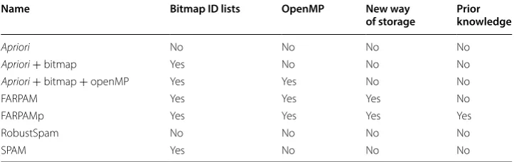
highly optimised and parallelised for a modern standalone multicore workstation, thus avoiding security issues with transfer of confidential data onto a cluster. They are profiled for applications to (1) itemsets using the existing and highly optimised SPAM code, (2) time-series recorded with errors in timestamps using RobustSPAM. We show that they are both faster and better scalable than SPAM and RobustSPAM. Table  1 presents a summary of the algorithms we have developed (FARPAM and FARPAMp), their intermediate versions (Apriori, Apriori+bitmap and Apriori+bitmap+openMP ) and the methods we used for profiling and verifying

outputs (RobustSPAM and SPAM). Table 2 shows the levels of optimisation used in the algorithms (fully described in “Steps in constructing and optimising FARPAM” section). All algorithms presented in the table produce identical outputs (the list of frequent patterns found for a given level of support, and the frequency and ID

Table 1 Algorithms tested in the paper

Name Language Source Algorithm

Apriori C++ Present paper PM with uncertainty intervals

and temporal length restric-tion

Apriori+bitmap

Apriori+bitmap+openMP

FARPAM FARPAMp

RobustSpam Java [37] PM with uncertainty intervals

SPAM Java [8] SPAM

Table 2 Optimisation details of the tested algorithms

Name Bitmap ID lists OpenMP New way

of storage Prior knowledge

Apriori No No No No

Apriori+bitmap Yes No No No

Apriori+bitmap+openMP Yes Yes No No

FARPAM Yes Yes Yes No

FARPAMp Yes Yes Yes Yes

RobustSpam No No No No

of entries where they have been found) for the same problems. The algorithms are applied to a confidential social care dataset and to a publicly accessible meteorological dataset.

Methodology

Definitions and notations

Suppose we have m unique items and denote them as ij , j=1,. . .,m . According to [6] an itemset is a non-empty set of items and a sequence is an ordered list of item-sets. We may denote an itemset I by (i1,i2,. . .,in) , where ij is an item, and a sequence

S by s1,s2,. . .,sk , where sj is an itemset. If a sequence consists of n itemsets we call

it sequential pattern of lengthn or n-pattern. It is possible that the same itemset may appear several times in a pattern, e.g. s1,s2,s1,s3,s1,s1 . Note that the order of items

within an itemset is not important while the order of itemsets matters and sequences s1,s2,s1,s3,s1,s1 and s1,s1,s1,s1,s3,s2 are different.

A database D is formed of several records (sets of sequences). Each record is

allowed to have a different number of sequences. All these records can be enumer-ated as ρk , k=1,. . .,r . For the k-th record of D we can check if a given pattern p is

a subpattern of ρk . In such a way we may count the number of records containing the given pattern p. This number divided by the total number of records in the data-base is called the support for the pattern p. By a frequent pattern we mean a pattern whose support is not less than a given threshold σ (minimum support). Our problem

is to find all possible frequent patterns in the database D.

In this paper we consider datasets consisting of events rather than items or sequences of itemsets. Each event is a triple {e,ts,te} , where e is a coded item, [ts,te] is an interval during which the event is equally probable to occur (uncertainty interval).

Let a customer regularly buy grocery in a supermarket. Each transaction contains a set of purchased items and represents a single row in the dataset. If the exact time of purchase is not relevant we can apply a standard sequential pattern algorithm like SPAM to search for frequent patterns. However, in some problems the time relation between the transactions can be important.

A sequence ej1_,ej2_{,. . .,e}js of s events from database _D is called ordered if

An ordered sequence ej1_,ej2_{,. . .,e}js of s events from _D is called a pattern of length s or s-pattern if

In the case of no uncertainty, the size of interval [ts,j tej] is reduced to 0. Therefore tsj=tej ≡tj and pattern can be defined as an ordered sequence of events ej1,ej2,. . .,ejs .

If the exact time tj is not important we can sort the events in each row (see Definition 1) and apply traditional SPAM. FARPAM and FARPAMp suggested in this work are also applicable.

(1) ∀i=1,. . .,s tji

s ≤tsji+1

(2)

∀i=2,. . .,s τ ≡ sup k=1,...,i−1

Sequential patterns

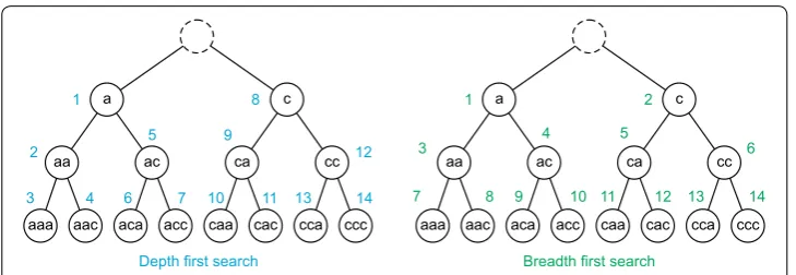
There are two main groups of sequential pattern mining algorithms: breadth first search (BFS) and depth first search (DFS). They come from methods used in artificial intelligence, e.g. [50], and depend on how a search tree is constructed. To explain the difference we consider an example in Fig. 1.

BFS methods suppose that all frequent patterns of a given length k are known, includ-ing where k=0 . We then search for (k+1)-patterns and once all those frequent pat-terns are found we search for (k+2)-patterns, and so on until all frequent patterns have been found. Classical examples of BFS methods can be Apriori-like algorithms first sug-gested in [5, 6] and based on ideas from the so-called Apriori Principle [51]: “All non-empty subsets of a frequent itemset must also be frequent”. BFS-like algorithms generate all k-patterns in each k-th iteration and move to the next k+1 step only after exploring

the entire k-th search space. This idea was later extended for the frequent itemset algo-rithm in [52–54] and for the case of constrained itemsets, in [55–57].

DFS methods, in contrast, construct the search tree by finding all frequent extensions of the current pattern before exploring other frequent patterns at the same level of the search tree, i.e. of the same length. The first DFS-like algorithm was suggested by intro-ducing the FP-grow method [13]. Subsequently, several improvements have been devel-oped, for example vertical representation of the database, or introduction of so called “TID-array” to link frequent itemsets to arrays of transaction IDs [58, 59]. In applica-tion to sequential pattern mining problems similar ideas were suggested in SPADE [7], SPAM [8], FreeSpan [9] and PrefixSpan [10]. Generally DFS methods are more difficult to parallelise.

The main disadvantage of BFS methods is related to memory usage, as a user needs to store all frequent k-patterns if any (k+1)-pattern is to be found. While memory require-ments for DFS algorithms can be less demanding compared to BFS, we may still need to store data related to all previous patterns, which can be challenging, especially when patterns are long. In this paper we only consider BFS methods.

Temporal data

It is often important to know not only the fact that an event ej took place but also the time tj at which it happened. We talk about a time series database when a sequence of events

{ej} is ordered according to their times tj . Temporal data may also have an interval-based c

a

aa ac ca cc

aac

aaa aca acc caa cac cca ccc

1

2

3 4 5

6 7 8

9

10 11

12

13 14

c a

aa ac ca cc

aac

aaa aca acc caa cac cca ccc

2 1

3 4 5 6

7 8 9 10 11 12 13 14

Depth first search Breadth first search

structure when an event happens between start ts and end te time points. Naturally, there

may be other types of temporal datasets, for example continuous functions of time. There are several ways to convert those functions into temporal datasets.

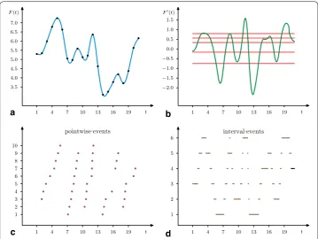
The following conversion procedure was used to generate events for the weather data-set (see “Evaluation” section for a full description). Suppose a variable F from the data-base can be written as a function F(t) of time. If the function is known at discrete time points only, e.g. as shown in Fig. 2a, we can use various interpolation techniques such as cubic spline interpolation. Let there be n time points ti , i=1,. . .,n , with known values

of F(t). We may use a cubic spline approximation _F(t)ˆ _{of F(t) given by functions Fi(t) for} each t∈ [ti,ti+1] , i=1,. . .,n−1:

As the values of F(t) are known at ti , we get Fˆi(ti)=F(ti) and Fiˆ(ti+1)=F(ti+1) ,

i=1,. . .,n−1 . We also require F(t)ˆ to have its first and second derivatives continuous at ti , i=1,. . .,n−2 : Fˆ_i′(xi+1)= ˆFi+′ 1(xi+1) , Fˆi′′(xi+1)= ˆFi′′+1(xi+1) . To have a unique solution we also put the following condition at the endpoints _Fˆ′′

1(x1)= ˆFn′′−1(xn)=0 .

Solving the system of linear equations we find the approximation _Fˆ_{(t) everywhere on} [t1,tn].

It is often necessary to preprocess the original data by some procedure. For instance, each patient may have their unique normal/abnormal values depending on their gender, age, or race. Therefore the original function should be scaled in order to get meaningful functions across many patients. In other cases we may use some values derived from the

(3)

ˆ

Fi(t)≡ai(t−ti)3+bi(t−ti)2+ci(t−ti)+di.

3.5 4.0 4.5 5.0 5.5 6.0 6.5 7.0

1 4 7 10 13 16 19 t 1 4 7 10 13 16 19 t

1 4 7 10 13 16 19 t 1 4 7 10 13 16 19 t

F(t)

−2.0 −1.5 −1.0 −0.5 0.0 0.5 1.0 1.5 F(t)

1 2 3 4 5 6 7 8 9 10

1 2 3 4 5 6

a _b

c _d

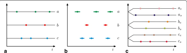
Fig. 2 Conversion of the continuous function F(t) into a time series of pointwise or interval based events. a Interpolation from a set of time points, b a derived function F′_{(t) with a set of levels important for the}

original function. As an illustration, we may measure wind speed at several locations. Clearly, some locations may be very windy, there can be strong seasonal variations and each place has its own wind rose showing how wind speed and direction are usually dis-tributed. So a normalisation procedure should be applied to the data, in order to know if wind speed has normal or extreme values for the chosen place and season. If we process temperature records, then it may be better to consider the first derivative F′(t) rather than absolute values F(t), see Fig. 2b. Now we need to convert the derived function into a set of temporal events, which can be done by introducing specific level values for the derived function [60]. We find time points when F′(t) intersects the given levels and take into account if the function is decreasing or increasing at those time points. Thus for 5 levels shown in Fig. 2b we get 2·5=10 events (5 for decreasing and 5 for increas-ing values) in Fig. 2c. On the other hand, we may also have interval based events when the function is between two levels (or above the highest/below the lowest levels), see 5+1=6 events in Fig. 2d.

Interval pattern mining problems can be challenging and take up a lot of time and data storage resources to solve, as various relations between any two time intervals should be considered. A simplified approach is to convert any interval-based event ej taking place within an interval [tsj,tej] into two events {esj,tsj} and {eje,tej} , where the superscripts s and e denote synthetic events corresponding to the beginning and end of the interval for event ej _{. In this way we should solve a the problem of pointwise time series events, see} exam-ples in [34–37]. A required sequential or time series pattern mining algorithm can be applied afterwards.

Uncertainty in data

There may be cases when we are not sure when a given event took place. For example, some health related measurements concerning a patient may be taken several times per day, while other procedures like CT/MRI/ultrasound can be performed less frequently due to their potential health hazards, costs or availability. The time taken to process and record results processing results may also differ, meaning that they may not be recorded in the order the actual measurements took place. Finally, there may simply be errors in transcribing manually collected data. All these issues introduce time uncertainty into the record. In the case of weather data some weather stations may have older equip-ment and report only daily values. These daily values allow us to roughly estimate when a given event took place, e.g. gale force winds started at 9 p.m., however there will be some uncertainty in our estimation, e.g. 3 h. Therefore we are given an approximate time tj with some uncertainty βj≥0 , so we are sure the event took place between ts and j tej

time points where tsj ≡tj−βj and tej ≡tj+βj . Parameter βj is allowed to be zero when

we know precisely when an event took place. Examples of databases with uncertainties can be found in [29, 37, 47].

Steps in constructing and optimising FARPAM

approach is based on a number of algorithmic advances (bitmap ID-lists, a special way of database representation, etc.) as well as multi-thread processing. To the best of our knowledge there is currently no parallelised algorithm that takes into account complex-ity introduced by uncertainty in datasets and temporal length restrictions on patterns.

We test our algorithms on two datasets: a weather dataset and an adult social care dataset. In the application to the adult social care dataset, we may want to look for fre-quent patterns where events happen over a certain period of time (for example, a few years). This restriction may help to reduce the number of frequent patterns used for the future classification or predictive models.

This section shows in details the modification steps we apply to the Apriori algorithm to achieve the final highly optimised FARPAM and FARPAMp. “Apriori principle” sec-tion describes the main principles of the Apriori algorithm (Algorithm 1). “Binary vec-tors” section shows modifications needed in order to achieve first-step optimisation. “Sorting frequent patterns” section talks about the way to accelerate the searching func-tion by sorting found frequent patterns. The implementafunc-tion of “ordering” the array of frequent s-patterns is described in “Forming a list of candidate patterns” section (Algo-rithm 2), its parallel implementation is shown on Fig. 4 and discussed in “ Multithread-ing” section. “Events with uncertainty intervals” section explains our approach to storing data and demonstrates how it works if applied to the datasets with uncertainty intervals. This is a universal method and can be applied to any dataset. Algorithms 4 and 5 present the method for searching for patterns in a dataset recorded in the our new format. This can be especially efficient for datasets with many repeated events. “Data with the same uncertainty for alike events” section shows how prior information can be used for fur-ther optimisation (implemented in FARPAMp). The searching function algorithm is pro-vided in Algorithms 6. “Time restriction” section explains how time restriction is put on a frequent pattern (Algorithm 7). The time restriction condition is implemented in both FARPAM and FARPAMp.

Apriori principle

For a standard Apriori-like approach each (s−1)-pattern p is extended by one event e, so a new candidate s-pattern p,e is formed (see for example [5]). Then for each record in the database D we check if the given s-pattern is a subpattern of the record. See

Algo-rithm 1 as an example algorithm to find frequent patterns. One can see that to find new patterns of length s we need to consider ns−1·n1 combinations, and for each combina-tion, all r records from database D should be considered. This can be time-consuming, so

we want to use the Apriori Principle in order to reduce the number of checks. Suppose a candidate s-pattern is a sequence ej1_,ej2_{,. . .,e}js . This pattern can be a subpattern of a given i-th record only when all its subpatterns are also subpatterns of the i-th record. By removing one event from the pattern ej1_,ej2_{,. . .,e}js we may form s subpatterns of length (s−1) , i.e. ej2_,ej3_{,. . .,e}js , _ej1_,ej3_{,. . .,e}js , _�ej1_,ej2_,ej4_{,. . .,e}js_{�,. . .,�e}j1_,ej2_,ej3_{,. . .,e}js−1_� . According to the Apriori Principle all these (s−1)-patterns must be subpatterns of the

input : A databaseD

input : A setFs−1of(s−1)-patterns,ns−1patterns in total input : A setF1of1-patterns,n1patterns in total

input : The minimum supportσ

output: A setFsofs-patterns,nspatterns in total setFsto the empty set;

ns←0;

foreachpatternpfromFs−1do foreachelementefromF1do

newCandidatePattern p, e;

κ←findSupport(newCandidatePattern, D); if κ≥σthen

addnewCandidatePatterntoFs;

ns←ns+ 1; end

end end

Algorithm 1:Apriori algorithm for breadth first search

Binary vectors

In order to use the Apriori principle we introduce a binary vector v of length r for each pattern p. An i-th element of this vector is 1 when the pattern p is a subpattern of the i-th record, otherwise vi=0 . Suppose a new candidate s-pattern p is given. By

pk , k=1,. . .,s we denote all its s subpatterns of length (s−1) and the corresponding

binary vectors are vk . If p is a subpattern of an m-th record of database D , then all

elements pm_k must be 1. Therefore we form a candidate binary vector v˜ such that ˜

vm_=vm

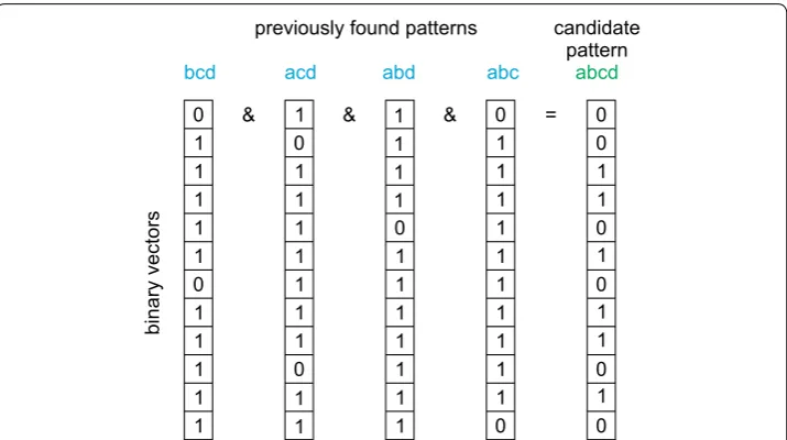
1 ∧vm2 ∧. . .vms where ∧ is the binary AND operator, see Fig. 3 for an example.

If the number of non-zero elements of vector v˜ is less than the minimum support σ ,

then the candidate pattern p will not be a frequent one. However, if the number of non-zero elements of v˜ is greater or equal to σ , then we need to check all records

correspond-ing to v˜m=1 . For example, pattern b,a,c,d,a,b,d,c contains subpatterns b,c,d , a,c,d , a,b,d and a,b,c , i.e. b_,a,c_,d_,a,b,d,c , _b,a_,c_,d_,a,b,d,c , _b,a_,c,d,a,b_,d_,c

and b,a_,c,d,a,b_,d_,c , however it does not contain pattern _a,b,c,d.

previously found patterns

bcd acd abd abc

0 & & & =

1 0 0 0 0 0 0 0 1 1 1 1 1 1 1 1 1 1 1 1 1 1 1 1 1 1 1 1 1 1 1 1 1 1 1 1 1 1 1 1 1 1 1 1 1 1 1 1 1 1 1 1 1 1 0 0 0 0 0 sr otc ev yr ani b candidate pattern abcd

Suppose we have N candidate records, i.e. records with v˜m=1 . We start processing them and count the number µ of records where p is not a subpattern of the record. Once 1−µ/N< σ , then there is no need to check the remaining records as the total number

of records with p as a subpattern will be less than σN and the candidate pattern p is not a

frequent one. Otherwise, after checking all the records we form the new binary vector v. For numerical implementation it is important to remember that a logical variable usu-ally requires at least 1 byte (8 bits) of memory. The use of logical variables for the vector

v will require 8 times more memory than is really needed. Therefore for a given number

r of records we can always assume that r is divisible by 32, otherwise we may create extra empty records to fulfil this assumption. So we can store a binary vector v in an r/32 long vector of 32-bit numbers. If m=32·M+i , where 0≤i<32 , then the element vm _is the i-th bit of the M-th 32-bit element in a storage system (we use C/C++ notations where the first element of a vector is stored at the 0-th position in memory). Then a bitwise AND operator can be applied to the corresponding M-th elements of vectors

v1,. . .,vs . The use of bitwise operators for 32-bit numbers instead of a logical operator

for 8-bit variables helps us not only to reduce the size of memory for data storage but also allows a CPU to issue 32 times less instructions. This idea resembles the bitmap ID list storage idea, first proposed in [8], and can be easily extrapolated to the case of sequential pattern mining.

If the number of records is large, then further steps for optimisation can be used. For instance, so called SIMD intrinsics (Single Instruction for Multiple Data) can be called when the same bitwise AND operator can be applied to an 128-, 256- or 512-bit number in one instruction

thus possibly saving processing time by up to a further 4, 8 or 16 times depending on the CPU type. However, in many cases there may be no need for low level optimisation as modern C/Fortran compilers may optimise a code themselves if they are aware of the number r of records for each vector v and the alignment of the vector in global memory.

Sorting frequent patterns

Suppose we have constructed the set F_s−1 of frequent patterns and a new candidate pat-tern p of length s is formed. By pk , k=1,. . .,s we denote subpatterns of p such that

pk is a pattern p without the k-th element. To apply the procedure described above we

need to find the corresponding binary vectors for all s subpatterns p_k . If at least one of the subpatterns does not belong to F_s−1 the candidate pattern p does not belong to Fs . It may happen that in a real application the number of patterns in F_s−1 is relatively large, i.e. thousands or millions of patterns. Therefore we need a smarter approach to finding the position of pk within the set Fs−1.

We aim to order patterns in Fs using lexicographical ordering. If _s=1 , then all pat-terns can be ordered according to the index of each event, i.e. ei <ej if i<j . For s>1 two different patterns p= �ei1,ei2,. . .,eis� and q= �ej1,ej2,. . .,ejs_� can also be ordered.

(4)

_mm_and_si128 (__m128i a, __m128i b),

_mm256_and_si256 (__m256i a, __m256i b),

We denote p<q if there is a number m≥1 such that eik _=ejk _{for k=1,. . .,m−1} and eim_<ejm (or in an equivalent manner _i

m<jm ). Suppose all patterns in the origi-nal sets F₁ and F_s−1 are ordered in Algorithm 1. Then the search for a pattern p in F_s−1 can be significantly accelerated if bisection-type algorithms are used. Other types of searching algorithms which can also be used are described in [61].

Multithreading

Modern CPUs offer the possibility to run on several threads at a time in parallel. To adapt the above algorithm to this situation, we propose two steps to find a new set Fs of frequent s-patterns. Firstly we generate possible candidate patterns and corre-sponding binary vectors as shown in Fig. 3. Secondly we check if a given candidate pattern is really a frequent pattern. The reason for splitting the original algorithm is to allow all threads to have a roughly uniform load for the search and checking steps. It may happen that some events occur more often than others, therefore a new candi-date p,e formed from a “more frequent” pattern p (with higher support values) may have a greater chance to be also a frequent pattern compared to a “less-frequent” pat-tern p (with values close the minimum support σ).

The simplest way to achieve multithreading is to give each thread a pattern p

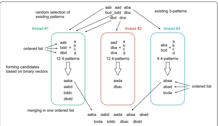
from F_s−1 and allow it to form all various combinations _p,e where e is a frequent 1-pattern from F₁ . Once a thread has processed all these possible patterns p,e , then a new (s−1)-pattern p is taken from the ordered set F_s−1 (see an example in Fig. 4 and details in Algorithm 2). As result each thread forms an ordered subset of Fs of candidate patterns. Due to parallel jobs we cannot put the candidate patterns in one set as this set may not be the ordered one. However, merging the resulting subsets into one can be done easily after all the threads finish their jobs because the subsets are ordered (see Algorithm 3).

aab aad aba bcd bdd dba dbd dca

existing 3-patterns

thread #1 thread #2 thread #3

random selection of existing patterns

forming candidates based on binary vectors

ordered list

ordered list

aaba aabd aada abaa abad

bddc dbac dbdd

bcda aab

bdd dbd

a b c d ×

12 4-patterns

aaba aabd bddc dbdd

aad dba dca

a b c d ×

12 4-patterns

aada dbac

aba bcd

a b c d ×

8 4-patterns

abaa abad bcda

merging in one ordered list

Once the final set of candidate patterns has been formed, the process of checking if a given pattern is a frequent one is straightforward to parallelise by giving each thread one or several patterns from the set of candidate patterns.

Events with uncertainty intervals

Suppose that each event is equally likely to happen in time interval [ts,te] , where ts and te are start and end points of the interval respectively. Thus each record becomes a list

of triples {ek,t_sk,t_ek} (in the interests of brevity we denote them as Ek ). We may say that a list {ek,t_sk,t_ek} , k=1,. . .,n forms an interval based sequence if there are n time points tk _{∈ [t}k

s,tek] such that tk ≤tk+1 , k=1,. . .,n−1. If there are two triples Ek ≡ {ek_,tk

s,tek} and Em≡ {em,tsm,tem} , we may order these

events:

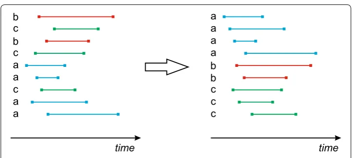
For our algorithms (FARPAM and FARPAMp) we decided to reorder all records accord-ing to the above definition. An example of such reorderaccord-ing is shown in Fig. 5. So 9 triples

can be reordered to form {a, 14.3, 18.4}_<{a, 14.9, 20.6}_<{a, 15.5, 17.6}_<{a, 16.5, 24.0} <{b, 15.6, 23.4}_<{b, 16.4, 20.8}_<{c, 15.2, 20.3}_<{c, 15.9, 19.4}_<{c, 17.2, 21.9}. For the implementation of the algorithm we store the following data for each record:

1. A total number of different events n (for the above example we have three different events ej , i.e. a, b and c);

2. A list of ordered events or their indexes, i.e. (a, b, c) or (1, 2, 3);

3. An array of start times, i.e. (14.3, 14.9, 15.5, 16.5, 15.6, 16.4, 15.2, 15.9, 17.2); 4. An array of end times, i.e. (18.4, 20.6, 17.6, 24.0, 23.4, 20.8, 20.3, 19.4, 21.9);

(5) Ek <Em if





ek <em,

ek _=em_andtk s <tsm,

ek =emandt_sk =t_smandt_ek <t_em.

(6)

{b, 15.6, 23.4},{c, 17.2, 21.9},{b, 16.4, 20.8},{c, 15.2, 20.3},{a, 14.3, 18.4}, {a, 15.5, 17.6},{c, 15.9, 19.4},{a, 14.9, 20.6},{a, 16.5, 24.0}

a

a

a

a

b

b

c

c

c

time

time

a

a

a

a

b

b

c

c

c

5. An (n+1)-array ξk of indexes to know what elements of start/end times are related to a given event (in our case it is ξ =(1, 5, 7, 10) ; so times for the second event

(which is b) are from ξ2=5 and till ξ3−1=7−1=6).

Data with the same uncertainty for alike events

Suppose a given pattern contains nalike events (events, which are coded by the same symbol or number) and a given record has m entries (for example, in Fig. 5 shows 4 events a, 3 events c and 2 events b). The procedure above requires us to check n per-mutations of m, i.e. m!/(m−n)! . For long records with many entries of same elements this can be very time-consuming. However, for some problems we may have extra prior information about time intervals. Suppose that for each event e any two time intervals [t_si,t_ei] and [ts,j tej] related to this event are ordered in the following way:

For example if alike events have the same uncertainty β , then we know for sure an event

takes place in the interval [˜ti_−β,˜ti_{+β] , so if we set t}i

s≡ ˜ti−β and tei ≡ ˜ti+β , then any two alike events can be reordered so to fulfil statement (7).

Assumption (7) leads to the fact that only permutations with tsj>ts for i j>i should be considered. Suppose we considered only ordered time intervals (i.e. satisfying 7) and have tried and failed to find a pattern in a record. If we permute any two entries of the alike event, then τ [as defined in (2)] for the new combination will be greater for some elements than τ found for the original combination and the requirement for τ ≤tej may

not be true.

In the case of ordered events we need to check m!/((m−n)!n!) patterns, i.e. the num-ber of n combinations from a set of m elements. Thus we need to process n! times less patterns compared to a general case. The procedure is shown in Algorithm 6.

Time restriction

For some practical problems it is important to not only find a given pattern for each client but also to be sure that all these events took place within a given time interval. This may help to exclude distant events which are not related to each other. If we set a time restriction interval T , then a list {ek,t_sk,t_ek} , k=1,. . .,n forms an interval based sequence with time restriction T if there are n time points tk ∈ [t_sk,t_ek] such that tk _≤tk+1 _{, k=1,. . .,n−1 and t}n_−t1_{≤T . Only small modifications of general} and ordered events in Algorithms 5 and 6 are required, see for instance Algorithm 7 for ordered events.

Main algorithms used in FARPAM Forming a list of candidate patterns

Let there be a database with n1 records. Suppose on a previous (s−1)-step we have found r frequent patterns of length (s−1) . We keep these frequent patterns in

r×(s−1)-matrix allPreviousPatterns. In fact this 2D matrix is stored as a 1D array by concatenating neighbouring rows of the matrix.

(7)

input :r: number of(s−1)-patterns found on the previous step input :n: number of frequent events

input :σ: minimum support

input : allPreviousPatterns: an array storing all(s₋1)-patterns

input : tempPattern: ans×(s−1)-matrix to store(s−1)-subpatterns of a temporary pattern for the given thread

input : indexOfPreviousPatterns: ans-array to store position of(s−1)-subpatterns input : binPrevious: an array with all binary vectors found on the previous step input : binTemp: a temporary array to store binary vectors for the given thread output:q: number of candidate patterns found for the given thread

output: binCandidate: an array with all new binary vectors found for the given thread output: candPattern: an array with candidate patterns found for the given thread q←0;

forifrom1tordo

/* all numbers from 1 to r are distributed between all threads */

/* Prefilling tempPattern array */

copyi-th(s−1)-array from allPreviousPatterns to the last row of tempPattern; forkfrom1tos−1do

copy1, . . . , k−1, k+ 1, . . . s−1elements of the last row of tempPattern to1, . . . s−2 elements ofk-th row respectively;

end

/* by the above procedure we have filled in all elements of tempPattern matrix except last in row elements for the top s−1 rows */ forjfrom1tondo

/* considering all frequent events */

set all last in row elements (for the top (s-1) rows) of tempPattern toj; formfrom 1 tosdo

indexOfPreviousPatterns[m]← position ofm-th row of tempPattern within allPreviousPatterns;

if indexOfPreviousPatterns[m] = 0then

/ * d e r e d i s n o c e b o t t n e m e l e t n e u q e r f t x e n e h t * /

breakm-loop and go thej-loop; end

end

copyindexOfPreviousPatterns[1]-th binary vector from binPrevious to binTemp; formfrom2tosdo

binTemp← bitwise AND for binTemp andindexOfPreviousPatterns[m]-th binary vector from binPrevious;

nb←numberOfNonZeroBits(binTemp); if nb< σrthen

breakm-loop and go thej-loop; end

end end

/* The new candidate pattern is found */

q←q+ 1;

save the last row of tempPattern as theq-th pattern of candPattern; save binTemp toq-th vector of binCandidate;

end

Algorithm 2:Forming a list of candidate patterns (parallel implementation)

For each pattern we keep a binary vector of length n1 , so each for each i-th record the corresponding element of the binary vector is 1 when the given pattern is present in the record, otherwise we set it to 0. In order to exploit SIMD features of modern processors it is better to assume that the number n1 of records is divisible by 32. We may always do so by adding extra (empty) records in the database. If we denote n32=n1/32 , then each binary vector can be stored as an n32-vector of 32-bit unsigned integer numbers. We place all binary vectors for r patterns in an array binPrevious of 32-bit unsigned integer numbers. The size of the array is n32×r.

frequent. Therefore we create a template s×(s−1)-matrix with each row consisting of elements of those (s−1)-subpatterns. In this matrix only the last element of first (s−1) rows are changed when we vary the extra event.

Once the template matrix is filled in for a given extra event, we check if all rows of the matrix are among the frequent patterns found on the previous step. If at least one of the patterns is missed, then the new s-pattern cannot be frequent and we should take another extra element and reiterate the procedure. In case of all rows of the matrix to be frequent, we find the corresponding binary vectors in binPrevious array. Those

s binary vectors are logically multiplied and the new binary vector for the candidate

s-pattern is formed. By counting the number of non-zero elements of the new binary vector we check if it is more or equal to σr where σ is the minimum support. Otherwise

the candidate pattern cannot be frequent.

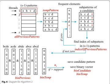
If there are several threads available, then all r patterns from the previous steps can be processed concurrently, e.g. with parallel for loop from OpenMP. The algorithm and its example diagram are presented in Fig. 6 and Algorithm 2.

We store (s−1)-subpatterns to form a candidate pattern in s×(s−1)×t-matrix tempPattern, where t is the number of threads. Every subpattern of a candidate can be described by its position in allPreviousPatterns. We store these positions in matrix indexOfPreviousPatterns. The size of matrix is t×s . When calculating

the binary vector for a candidate we store it in binTemp. The size of it is n32 . After doing all the steps in Algorithm 2 we store the binary vector of a candidate and the candidate pattern itself in matrices binCandidate and candPattern. The size of binCandi-date is n32×100, 000 . Size of candPattern is (s−1)×100, 000 . We chose 100, 000 as an upper limit of maximum number of candidates (can be changed if it is needed).

1 2 r threads (s-1)-patterns a b c d ... ... ... ... ... ... frequent elements a b c d

a b c db c a

a b a c

subpatterns of a candidate

find index of subpattern b c d

d d

a b c db c a

a b a c b c d

d d e in (s-1)-patterns ore zfi

if not zero

bcde acde abde abce abcd

0 0 1 1 1 1 0 1 1 1 0 0 1 1 1 0 1 1 1 0 1 0 0 1 1 1 0 0 1 1 1 1 0 0 0 & & & &

if > support

save candidate pattern save binary vector

e ee

e allPreviousPatterns tempPattern indexOfPreviousPatterns binPrevious binTemp 0 0 1 0 1 0 0 n_b binCandidate binTemp

Merging candidate patterns

Suppose that n OpenMP threads are used and m frequent candidate s-patterns are found. Each thread stores all candidate patterns it has found in its own block of mem-ory. In principle, the corresponding binary vectors can be stored in a common block of memory thus avoiding extra data copying. In our algorithm we prefer to store all pat-terns as a lexicographically ordered list. This type of storage allows us to check in a faster way if a given pattern belongs to the list. Otherwise one needs to check all patterns in the list when searching for (s−1)-patterns. As each thread processes (s−1)-patterns from the ordered list by concatenating with single events also from the lexicographically ordered list of 1-patterns, then the candidate patterns found by this thread will also form a lexicographically ordered list of s-patterns. Thus we just need to merge n ordered lists found by n threads.

input :s: size of patterns

input :n: number of arrays ofs-patterns input :vk: thek-th ordered array ofs-patterns input :qk: size ofvk

input :Ψ: a large integer number (more than the number of frequent events) output:w: output ordered array ofs-patterns

output:m: size of the output array m←0;

forkfrom1tondo

m←m+qk;ηk←1; /* index of the current pattern in the k-array */ end

forpfrom1tomdo µ←0;

forifrom1tosdo

ui_{←Ψ; /* set all elements of the ‘‘smallest’’ pattern to the largest} number */

end

forjfrom1tondo ifηj> qjthen

/* all elements from the j-th array have been considered; we should

consider the next array */

continue; end

isBetter←true;

β←the pointer to theqj-th pattern of thej-th array; forlfrom1tosdo

ifβl_{> u}l_then

isBetter←false;

break; end

ifβl_{< u}l_thenbreak; end

ifisBetter = falsethencontinue;

µ←j;

forlfrom1tosdo ul_←βl_; end end

adduto the arrayw; ηµ←ηµ+ 1; end

We define an array of frequent patterns found by a single OpenMP k-th thread as vk and the corresponding size of the array as qk . Algorithm 3 shows how found frequent patterns are merged into output array ω of frequent s-patterns (all resultant patterns

become sorted).

The total number of candidate patterns is m=n

k=1qk . For each n list of ordered patterns we store the index of the smallest pattern (not yet merged to the final list), we denote it as η_k and set to 1 initially.

We introduce a working s-vector u. For each new ordered s-pattern to be found from the given n lists we initially set all elements of u to (a number larger than the number

of events). Then for each n lists we consider smallest patterns not yet merged, i.e. ηk-th

pattern for the k-th list. By comparing the working vector u with corresponding n small-est patterns we find the index µ of the smallest of them. Then we put the found pattern to the merged list and increment ηµ by 1.

Note that due to the process of formation of candidate patterns each n lists of patterns does not have any common s-patterns with the other n−1 lists. This allows us to slightly

reduce the number of checks compared to a general case of merging patterns with pos-sibly common patterns.

Checking if a subpattern belongs to a record (initialisation step)

The Algorithm 4 shows the initialisation part of a searching function (used in FARPAM). Each event is defined as a triple of event index, start and end times. Suppose a record consists of m events. All those events can be sorted according to rule (5). Therefore we get n distinctive events ( n≤m ) and two m-arrays for the start/end times of the events.

input :p: the givens-pattern

input :n: number of distinctive events in a record input :q: an array of the distinctive events

input :ξk_{: an array of start positions for all events related toq}k_event input :ts/te: an array of start/end times for each event

output: true/false: true if the given pattern is found forifrom1tosdo

τ←false;

forjfrom1tondo if pi_=qj _{thencontinue;} τ←true;

vFirst[i]←ξj_{;vLast[i]←ξ}j+1_−1;

/* start/end positions of data related to pi _{event in the given record */} break;

end

if τ= falsethenreturnfalse;

end

/* setting the start position for each event */

forifrom1tosdo

vCurrent[i]←vFirst[i]; end

/* finding the index of same previous/next events if they exist, otherwise 0 */ forifrom1tosdo

previousIndex[i] = 0;

nextIndex[i] = 0; end

forifrom2tosdo

forjfromi−1to1by−1do if vFirst[i] = vFirst[j]then

previousIndex[i] =j;nextIndex[j] =i; break;

end end end

/* in case of several same events we need to adjust start positions */ forifrom2tosdo

if previousIndex[i] = 0thencontinue;

vCurrent[i] = vCurrent[previousIndex[i]] + 1;

if vCurrent[i]>vEnd[i]thenreturnfalse; end

Algorithm 4: Checking if a given pattern is a subpattern for a given record (initialisation step)

We aim to consider all possible combinations of events. For the event pi we keep its position within the record as an index vCurrent[i] which can have values between vFirst[i] and vLast[i]. It is clear that in case of two same events pi and pj they

cannot point to the same event in the record. Therefore we want to avoid cases when two positions vCurrent[i] and vCurrent[j] are the same. Therefore in the example above we cannot set vCurrent = {1,3,3,6,3} as the second, third and

fifth events point to the third element. Thus for the initialisation step in this algorithm for each element we first find previous/next alike elements previousIndex and nextIndex if they exist and reset current values based on values of previous elements. It is clear that the index vCurrent[i] should not exceed the index of the last alike element. The algorithm takes into account cases when there are more alike events in a given pattern than in a record (and returns false).

• Initial values: {7, 8, 9}.

• Now we increment the third element by one and get {7, 8, 10} , this element is greater than vLast[3]=9 , so we set {7, 9, 7} . The first and the last elements are the same, so we set {7, 9, 8}.

• By incrementing the third element by one we get {7, 9, 9}, so by cor-recting out-of-range and identical values we get this procedure {7, 9, 9} → {7, 9, 10} → {7, 10, 7} → {8, 7, 7} → {8, 7, 8} → {8, 7, 9}.

• In a similar way {8, 7, 10} → {8, 8, 7} → {8, 9, 7}_.

• {8, 9, 8} → {8, 9, 9} → {8, 9, 10} → {8, 10, 7} → {9, 7, 7} → {9, 7, 8}. • And the final vector {9, 7, 9} → {9, 7, 10} → {9, 8, 7}.

So we have to check 3!/(3−3)! =3!/0! =6/1=6 patterns.

Of course, checking all m!/(m−n)! is the worst case scenario and is not always the case (since all our events are rearranged according to rule 5). However, pattern cacc in the record

will require to check all the possible combinations, starting from vCurrent= {2, 1, 3, 4} , and ending with vCurrent= {4, 1, 3, 2} as a solution.

Checking if a subpattern belongs to a record (iteration step)

For the second (iteration) step we suppose a valid combination of vCurrent[i] is given, i.e. vCurrent[i] =vCurrent[j] for any i =j (for example, vCurrent= {1, 1, 1} is not valid while vCurrent= {1, 3, 2} is). Let us have a record with Ei ≡ {ei,t_si,t_si} and Ej≡ {ej,tsj,ts}j , and want to check if pattern (ei,ej) can be a sub-pattern in the record. We need that ti≤tj where ti∈ [t_si,t_ei] and tj∈ [tsj,tej] . This may

happen only if ti s≤t

j

e . The minimum possible value of ti _{is then ts and} i _tj _{may vary from} max(t_si,tsj) to tej . So if we introduce τ =ts1 for the first element in the pattern, then we

should check that for each following element of the pattern τ ≤tej and re-define τ as

max(τ,tsj) . If we succeed to fulfil these requirements for a given s-vector of indexes vCurrent[i], then the subpattern is found, otherwise we need to check the next per-mitted combination of indexes vCurrent[i], see Algorithm 5.

repeat

τ←vStartTime[vCurrent[1]];J←0;

forifrom2tosdo

I←vCurrent[i];

if τ >vTimeEnd[I]then

J←I; break; end

τ←max(τ,vStartTime[I]);

end

if J= 0thenreturntrue;

is←vFirst[J];ie←vLast[J];

/* create a list of previous alike events */

u←previousIndex[J];numberOfPreviousEvents←0;

whileu >0do

poistionOfPrevious[numberOfPreviousEvents]←vCurrent[u];

numberOfPreviousEvents←numberOfPreviousEvents + 1;

u←previousIndex[u];

end

N←1;

repeat

b= false;

vCurrent[J]←vCurrent[J] + 1;

if vCurrent[J]> iethen

if previousIndex[J] = 0thenreturnfalse;

J←previousIndex[J];N←N+ 1;b←true;

else

forifromNtonumberOfPreviousEventsdo

if vCurrent[J] = positionOfPrevious[i]then

b←true; break; end

end end untilb= false;

u←previousIndex[J];

N←1;

positionOfPrevious[1]←vCurrent[J];

whileu >0do

positionOfPrevious[N]←vCurrent[u];

N←N+ 1;u←positionOfPrevious[iu];

end

u←nextIndex[J];

whileu >1do

vCurrent[u]←is;

repeat

b←false;

forifrom1toNdo

if vCurrent[u] = poistionOfPrevious[i]then

vCurrent[u]←vCurrent[u] + 1;b←true;

break; end end untilb= false;

positionOfPrevious[N]←vCurrent[u];

N←N+ 1;u←nextIndex[u];

end untiltrue; returnfalse;

Algorithm 5: Checking if a given pattern is a subpattern for a given record (iteration step)

Ordered events

/* finding the index of the same previous event if it exists, otherwise 0 */ forifrom1tosdo

previousIndex[i]←0;

end

forifrom2tosdo

forjfromi−1to1by−1do

if vCurrent[i] = vCurrent[j]then

previousIndex[i]←j; break;

end end end

τ←vTimeStart[vCurrent[1]];

forifrom2tosdo

b←false;

if previousIndex[i]>0thenvCurrent[i]←vCurrent[previousIndex[i]] + 1;

repeat

J←vCurrent[i];

if vTimeEnd[J]≥τ then

τ←max(τ,vTimeStart[J]);

b←true; break; end

vCurrent[i]←vCurrent[i] + 1;

if vCurrent[i]≤vLast[i]thenbreak;

untilb = true; end

returntrue;

Algorithm 6: Checking if a given pattern is a subpattern for a given record (iteration step) for ordered events

whilevCurrent[1]≤vLast[1]do τ1= vTimeStart[vCurrent[1]]; τ2= vTimeEnd[vCurrent[1]]; forifrom2tosdo

vCurrent[i]←vFirst[i]; end

forifrom2tosdo b←false;

if previousIndex[i]>0thenvCurrent[k]←vCurrent[previousIndex[i]] + 1; whilevCurrent[i]≤vLast[i]do

J←vCurrent[i];

if vTimeEnd[J]> τ1then τ1←max(τ1,vStartTime[J]); τ2←min(τ2,vEndTime[J]); t←true;

break; end

vCurrent[i]←vCurrent[i] + 1; end

if τ1> τ2+ ∆Tthenbreak; if b= falsethenreturnfalse; if i=sthenreturntrue; end

vCurrent[1]←vCurrent[1] + 1; end

returnfalse;

Algorithm 7: Checking if a given pattern is a subpattern for a given record (iteration step) for ordered events with time restriction

Evaluation

Adult social care database

The database consists of approximately 100,000 adult social care records over a period of 15 years (also used in [37]). The records cannot be processed outside the secure facilities of Leeds Institute for Data Analytics (LIDA) at the University of Leeds. After removing records with fewer than three events and selecting people within a certain age range the dataset was reduced to ≈25, 000 records. All the events have been cate-gorised and coded, where each code (event label) represents one of the following four event types: a referral to adult social care, an assessment, a service (including reable-ment activity) or a review. Referral event codes are composed of three parts: source (who made the referral)—2 categories; reason (why the service is needed)—12 catego-ries and outcome (decision for assessment)—15 categocatego-ries. The assessment activity is coded using only one variable; eligibility with 16 categories. The service activity is coded with 116 categories and the review activity with 17 categories. The final num-ber of unique codes (unique existing combinations of categories for all codes) is 301.

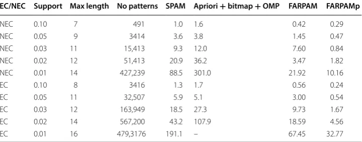
We consider an event of interest to be the use of a form of intensive, high cost care provision, a permanent residential or nursing placement, called for simplicity “Expen-sive Care” (EC in short), with the alternative event being called “Non Expen“Expen-sive Care” (NEC), which we use to split the clients into two groups: EC, with 6128 clients with 111,736 events in total and 252 unique events and NEC, with 18,518 clients, 286,201 total number of events, 258 unique events). It is clear that the average number of events per client in the EC group is much higher and we expect that the two groups will provide an interesting test bed for the performance of our algorithms. The out-put from our algorithm can be further used for risk stratification (see [37] for initial results using RobustSpam).

Each event is an interval that is represented with a starting time point and ending time point (together with the event label as discussed in “Methodology” section, see Fig. 7), the length of the interval varies and is even reduced to single points on some occasions. We allow an uncertainty β on the time stamp of the starting and

ending point events. β could depend on the type of event (for example, services

could be recorded with better accuracy than referrals) although here we consider uniform uncertainty. In principle, a frequent pattern mining algorithm can use prior information as in (7). However, in order to illustrate how prior information

t

a _b t _c t

a a

as ae

b b

bs be

c c

cs ce

can improve performance we apply both the general and ordered versions of the algorithm to this dataset (Algorithms FARPAM and FARPAMp correspondingly).

Weather dataset

To see how performance of the proposed algorithm may depend on various hardware parameters we decided to use a publicly available dataset. The European Commission provides access to weather data via Agri4Cast Resources Portal of the Joint Research Centre (http://agri4 cast.jrc.ec.europ a.eu). Gridded Agro-Meteorological database con-tains meteorological parameters from weather stations interpolated on a 25 ×25 km

grid. Meteorological data are available on a daily basis from 1975 to the last calendar year completed, covering the EU Member States, neighbouring European countries, and the Mediterranean countries. The following variables can be accessed:

• Maximum/minimum/mean temperature, • Mean daily wind speed at 10 m(m/s),

• Vapour pressure (hPa),

• Sum of precipitation (mm/day),

• Potential evaporation from a free water/crop canopy/moist bare soil surface (mm/ day),

• Total global radiation ( kJ/m2/day), • Snow depth.

We chose a mean daily temperature to generate patterns according to the procedure described in “Temporal data” section and shown in Fig. 2. As temperature has sea-sonal variation we consider its first derivative T′(t) . Suppose that for each grid point where data were interpolated from weather stations we have chosen nlevel levels Tj′ ,

j=0,. . .,nlevel−1 . Then j-th event happens at a time τk when T′(τk)=Tj and ′ T′′(τk)≥0

while (j+n_level)-th even happens if T′(τ_k)=Tj and ′ T′′(τ_k) <0 . So for each grid point

we have a sequence 2nlevel events. We chose Tj′ values in such a way, so T′(t)≤Tj′ for

(j+1)tmax/nlevel , j=0,. . .,nlevel−1 , time where tmax is the total period of time the given

variable is known (we used 20 years). Note that each grid point has its own values for T_j′. The weather data allows us to form various datasets. If we choose places in a rela-tively small region (one country like the UK), then we should expect a high level of correlation between temperature rise and fall for neighbouring places, thus we expect to have a lot of patterns even for large values of minimum support, e.g. σ =0.99 . On the other hand, temperature variations in the Mediterranean and Baltic countries may often behave independently. At the same time we may also control the length of patterns we aim to find. Each record corresponds to events that took place within a given time period. It is clear that during a 5-day period we get fewer events compared to a 25-day period. In this way we may control the maximum length of patterns for the given minimum support level.

Hardware

Two workstations were used to get performance results:

• WS4. CPU: Intel Core i7-4790 (codename Skylake, 4 cores, processor base frequency 3.6 GHz), RAM: 16 GB, operating system: 64-bit Windows 8.1. This workstation is a part of LIDA of University of Leeds where the private social care records can be pro-cessed.

• WS6. CPU: Intel Core i7-3930K (codename Sandy Bridge E, 6 cores, processor base frequency 3.2 GHz), RAM: 32 GB, operating system: 64-bit Windows 10. This work-station was used to process the weather dataset.

All codes were compiled with an Intel C++ compiler (part of Intel Parallel Studio XE

2016), in release mode, with maximum optimisation (favour speed, /O2 flag). For multi-threaded versions of the codes, OpenMP was used.

Results

We evaluate the efficiency of the proposed optimisation by comparing results with other existing algorithms where possible as well as by varying some parameters of the problems.

Sequential pattern mining

If the uncertainty parameter β is set to zero (and with the assumption that for each

record no two events happen at the same time), then the problem becomes a classical sequential pattern mining problem. Therefore we are able to compare results and per-formance of our optimised algorithms with other publicly available sequential pattern mining algorithms. We decided to use a SPAM code from SPMF (http://www.phili ppe-fourn ier-viger .com/spmf/, an open-source data mining library written in Java, [62]). This is considered to be one of the most efficient codes for sequential pattern mining prob-lems and according to [8] it outperforms such algorithms as SPADE and PrefixSpan. Our codes are written in C and compiled with an Intel C compiler. Of course, it is not fully correct to compare codes written in different languages, however our aim is simply to provide the reader with an idea of possible improvements. It is likely that direct conver-sion (without any optimisation) of a Java code to C or Fortran languages will provide a user with shorter run times (both implementations should have similar dependence on parameters of a problem, e.g. number of patterns or minimum support). In order to give a more realistic comparison for the C code we have implemented a naive version of the

Apriori-like algorithm with bitmaps similar to the method in [8].

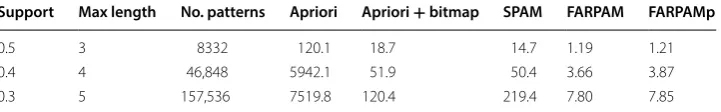
Table 3 Run times (in seconds) for algorithms with zero uncertainty β=0 for the weather

dataset (L3-D3-T14) measured over 14 places in the UK

Support Max length No. patterns Apriori Apriori+bitmap SPAM FARPAM FARPAMp

0.5 3 8332 120.1 18.7 14.7 1.19 1.21

0.4 4 46,848 5942.1 51.9 50.4 3.66 3.87