Open Access
Research article
Preparation of name and address data for record linkage
using hidden Markov models
Tim Churches*
1
, Peter Christen
2
, Kim Lim
1
and Justin Xi Zhu
2
Address: 1Centre for Epidemiology and Research, Public Health Division, New South Wales Department of Health, Locked Mail Bag 961, North
Sydney 2059, Australia and 2Department of Computer Science, Australian National University, Canberra, Australia
Email: Tim Churches* - [email protected]; Peter Christen - [email protected]; Kim Lim - [email protected]; Justin Xi Zhu - [email protected]
* Corresponding author †Equal contributors
Abstract
Background: Record linkage refers to the process of joining records that relate to the same entity or event in one or more data collections. In the absence of a shared, unique key, record linkage involves the comparison of ensembles of partially-identifying, non-unique data items between pairs of records. Data items with variable formats, such as names and addresses, need to be transformed and normalised in order to validly carry out these comparisons. Traditionally, deterministic rule-based data processing systems have been used to carry out this pre-processing, which is commonly referred to as "standardisation". This paper describes an alternative approach to standardisation, using a combination of lexicon-based tokenisation and probabilistic hidden Markov models (HMMs).
Methods: HMMs were trained to standardise typical Australian name and address data drawn from a range of health data collections. The accuracy of the results was compared to that produced by rule-based systems.
Results: Training of HMMs was found to be quick and did not require any specialised skills. For addresses, HMMs produced equal or better standardisation accuracy than a widely-used rule-based system. However, acccuracy was worse when used with simpler name data. Possible reasons for this poorer performance are discussed.
Conclusion: Lexicon-based tokenisation and HMMs provide a viable and effort-effective alternative to rule-based systems for pre-processing more complex variably formatted data such as addresses. Further work is required to improve the performance of this approach with simpler data such as names. Software which implements the methods described in this paper is freely available under an open source license for other researchers to use and improve.
Background
IntroductionRecord linkage refers to the process of joining records that relate to the same entity or event in one or more data col-lections [1]. The entity is often a person, in which case record linkage may be used for tasks such as building a
longitudinal health record [2], or relating genotypic infor-mation to phenotypic inforinfor-mation [3,4]. In other settings, the aim may be to link several sources of information about the same event, such as police, accident investiga-tion, ambulance, emergency department and hospital ad-mitted patient records which all relate to the same motor Published: 13 December 2002
BMC Medical Informatics and Decision Making 2002, 2:9
Received: 29 October 2002 Accepted: 13 December 2002
This article is available from: http://www.biomedcentral.com/1472-6947/2/9
vehicle accident [5]. Record linkage (originally known as "medical record linkage") is now widely used in research – in October 2002, a search of the biomedical literature via PubMed for "medical record linkage" as a Medical Subject Heading returned over 1,300 references [6].
The process of record linkage is trivial where the records that relate to the same entity or event all share a common, unique key or identifier – an SQL "equijoin" operation, or its equivalent in other data management environments, can be used to link records. However, often there is no unique key which is shared by all the data collections which need to be linked, particularly when these data col-lections are administered by separate organisations, possi-bly operated for quite different purposes in disparate subject domains.
In these settings, more specialised record linkage tech-niques need to be used. These techtech-niques can be broadly divided into two groups: deterministic, or rule-based tech-niques, and probabilistic techniques. A full description of these techniques is beyond the scope of this paper. A number of recent reviews of this topic are available [7,8]. However, all of these techniques rely on an element-wise comparison between pairs of records each comprising an ensemble of non-unique, partially identifying personal (or event) attributes. These attributes commonly include name, residential address, date of birth (or age at a partic-ular date), sex (or gender), marital status, and country of birth.
For example, consider the fictitious personally-identified records in Table 1.
The evident variability in the formatting and encoding of these records is quite typical of data collections which have been assembled from multiple sources. This variabil-ity tends to frustrate naive attempts at automated linkage of these records. To a human, it is obvious that records 0 and 2 represent the same person. It is quite likely, but not certain, that records 1 and 3 also represent the same per-son. The status of record 4 with respect to records 0 and 2 is far less clear – could this be Gwendolynne's spouse, Eve-lyn, or is this Gwendolynne with her sex and age wrongly recorded?
Regardless of the method used to automate such deci-sions, it is clear that transformation of the source data into a normalised form is required before valid and reliable comparisons between pairs of records can be made. Such transformation and normalisation is usually called "data standardisation" in the medical record literature, and "da-ta cleaning" or "da"da-ta scrubbing" in the computer science literature. We will refer to the process as "standardisation" henceforth, which should not be confused with the
epide-miological technique of "age-sex standardisation" of inci-dence or prevalence rates.
Standardisation of scalar attributes such as height or weight involves transformation of all quantities into a common set of units, such as from British imperial to SI units. Categorical attributes such as sex are usually trans-formed to a common set of representations through sim-ple look-up tables or mapping of various encodings – for example, both "Female" and "2" might be mapped to "F" and "male and "1" to "M" in order to provide a consistent encoding of the sex attribute for each record. Such trans-formations do not present a major challenge. However, standardisation of attributes which are recorded in highly variable formats, such as names or residential addresses, is far less straightforward, and it is with this task that this pa-per is concerned.
This standardisation task can itself be decomposed into two steps: segmentation of the data into specific, atomic data elements; and the transformation of these atomic el-ements into their canonical forms. In some cases, a third step, the imputation of missing or blank data items, and a fourth step, the enhancement of the original data with known alternatives, may also be required.
Some examples of the first two steps will make this clearer. Table 2 shows the segmented and transformed forms of the name, address and sex attributes of the illustrative records introduced in Table 1.
Once the original data have been segmented and stand-ardised in this way, further enhancement of the data is possible. For example, missing postal codes and territories can be automatically filled in from reference tables, and alternate, canonical forms of names can be added where informal, anglicised or other known variations are found, such as "Angie" (Angela, Angelique) or "Lyn" (Evelyn, Lyndon).
Related work
The most common approach for name and address stand-ardisation is the manual specification of parsing and transformation rules. A well-known example of this ap-proach in biomedical research is AutoStan, which was the companion product to the widely-used AutoMatch proba-bilistic record linkage software [10].
AutoStan first parses the input string into individual words, and each word is then mapped to a token of a par-ticular class. The choice of class is determined by the pres-ence of that word in user-supplied, class-specific lexicons (look-up tables), or by the type of characters found in the word (such as all numeric, alphanumeric or alphabetical). An ordered set of regular expression-like patterns is then evaluated against this sequence of class tokens. If a class token sequence matches a pattern, a corresponding set of actions for that pattern is performed. These actions might include dynamically changing the class of one or more
to-kens, removing particular tokens from the class token se-quence, or modifying the value of the word associated with that token. The remaining patterns are then evaluat-ed against the now modifievaluat-ed class token sequence – in other words, the pattern matcher is re-entrant, and the ac-tions associated with more than one pattern may act on any given token sequence. When the evolving token se-quence for a particular record has been tested against all the available patterns, the words in the input string are output into specific fields corresponding to the final class of the tokens associated with each word.
Such approaches necessarily require both an initial and an ongoing investment in rule programming by skilled staff. In order to mitigate this requirement for skilled program-ming, some investigators have recently described systems which automatically induce rules for information
extrac-Table 1: Some illustrative, fictitious, personally-identified records
Record Number Name Sex Street address Locality Age in years
0 Gwen Palfree F Flat 17 23–25 Knitting
Street
West Wishbone 2987 New South Wales
42
1 Angie Tantivitiyapitak F Wat Paknam Saint George Ave
Old Putney NSW 2345
27
2 Gwendolynne Palfrey 2 17/23 Knitting St Wishbone West NSW 2987
42
3 Tontiveetiyapitak, Angela
Female C/- Paknam Monas-tery, 245 St George St
Putney 2345 28
4 Palfrey, Lyn 1 Corner of Knitting
and Cro
chet Streets, Wish-bone New Sth Wales
43
Note: The "bleeding" of street address data into the locality column in record 4 is deliberate, and typical of real-life data captured by information systems with fixed-length data fields.
Table 2: Segmented and transformed versions of the records from Table 1
Data element Record 0 Record 1 Record 2 Record 3 Record 4
Given names gwen angie gwendolynne angela lyn
Surnames palfree tantivitiyapitak palfrey tontiveetiyapitak palfrey
Sex female female female female male
Institution names paknam paknam
Institution types monastery monastery
Unit types flat
Unit identifiers 17 17
Wayfare numbers 23,25 23 245
Wayfare names knitting saint george knitting saint george knitting, crochet
Wayfare types street avenue street street street
Wayfare qualifier corner
Locality name wishbone putney wishbone putney wishbone
Locality qualifiers west old west
Territories nsw nsw nsw nsw
tion from unstructured text. These include Whisk [11], No-dose [12] and Rapier [13].
Probabilistic methods are an alternative to these deter-ministic approaches. Statistical models, particularly hid-den Markov models, have been used extensively in the computer science fields of speech recognition and natural language processing to help solve problems such as word-sense disambiguation and part-of-speech tagging [14]. More recently, hidden Markov and related models have been applied to the problem of extracting structured infor-mation from unstructured text [15–20].
This paper describes an implementation of lexicon-based tokenisation with hidden Markov models for name and address standardisation – an approach strongly influ-enced by the work of Borkar et al. [20]. This implementa-tion is part of a free, open source [21] record linkage package known as Febrl (Freely extensible biomedical record linkage) [22]. Febrl is written in the free, open source, object-oriented programming language Python
[23]. Other aspects of the Febrl project will be described in subsequent papers.
Cleaning and tokenisation
The following steps are used to clean and tokenise the raw name or address input string. Firstly, all letters are convert-ed to lower case. Various sub-strings in the input string, such as " c/- " or " c.of " are then converted to their canon-ical form, such as "care_of ", based on a user-specified and domain-specific substitution table. Similarly, punctuation marks are regularised – for example, all forms of quota-tion marks are converted to single character (a vertical bar). The cleaned string is then split into a vector of words, using white space and punctuation marks as delimiters.
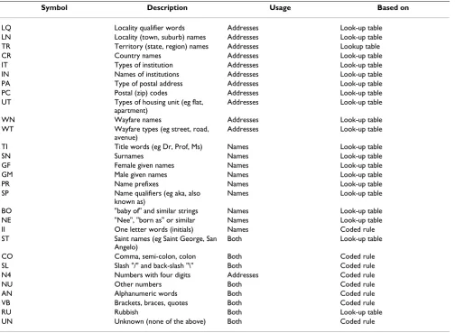
Using look-up tables and some hard-coded rules, the words in this input vector are assigned one or more to-kens, to which we will refer as "observation symbols" henceforth. The hard-coded rules include, for example, the assignment of the AN (alphanumeric) observation symbol to all words which are a mixture of alphabetic and numeric characters. However, the majority of observation symbols are assigned by searching for words, or sub-se-quences of words, in various look-up tables. A list of the observation symbols currently supported by the Febrl
package is given in Table 3. For example, one of the look-up tables may be a list of locality names. If a word (or con-tiguous group of words) is found in the locality table, then the LN (locality name) observation symbol is assigned to that word (or group). This look-up uses a "greedy" match-ing algorithm. For example, the wayfare name look-up ta-ble might contain a record for "macquarie", the locality qualifier look-up table might contain a record for "fields" and the locality name look-up table might contain a
record for "macquarie fields". If the first word in the input vector is "macquarie" and the second word is "fields", these first two words will be coalesced (into "macquarie_fields") and will be assigned an LN (locality name) observation symbol, rather than the first word be-ing assigned a WN (wayfare name) symbol and the sec-ond field an LQ (locality qualifier) symbol.
Such lexicon-based tokenisation allows readily-available lists of postal codes, locality names, states and territories, as typically published by postal authorities or government gazetteers, to be leveraged to provide the probabilistic model used in the next stage with the maximum number of "hints" about the semantic content of the input string. Note that these probabilistic models are able to cope with situations in which incorrect observation symbols are as-signed to particular words in the input string – the only re-quirement is that the symbols are assigned in a consistent fashion. For example, the input string "17 macquarie fields road, northmead nsw 2345" might be tokenised as "NU-LN-WT-LN-TR-PC" (number-locality name-wayfare type-locality name-territory-postal code). The first LN symbol is wrong in this context because "macquarie fields" is a wayfare name, not a locality name. The hidden Markov models described in the next section are readily able to accommodate such incorrect tokenisation.
Hidden Markov models
A hidden Markov model (HMM) is a probabilistic finite state machine comprising a set of observable facts or ob-servation symbols (also known as output symbols), a fi-nite set of discrete, unobserved (hidden) states, a matrix of transition probabilities between those hidden states, and a matrix of the probabilities with which each hidden state emits an observation symbol [24]. This "emission matrix" is sometimes also called the "observation matrix".
Training data are representative samples of the input records which have been tokenised into sequences of ob-servation symbols as described above, and then tagged with the hidden state which the trainer thought was most likely to have been responsible for emitting each observa-tion symbol. Maximum likelihood estimates (MLEs) are derived for the HMM transition and emission probability matrices by accumulating frequency counts for each type of state transition and observation symbol from the train-ing records. The probability of maktrain-ing the transition from state i to state j is the number of transitions from state i to state j in the training data divided by the total number of transitions from state i to a subsequent state. Similarly, the probability of observing symbol k given an underlying (hidden) state j is the number of times, in the training da-ta, that symbol k was emitted by state j divided by the total number of symbol emissions by state j. Because of the use of frequency-based MLEs, it is important that the records in the training data set are reasonably representative of the
data sets to be standardised. However, as reported below, the HMMs appear to be quite robust with respect to the training set used and quite general with respect to the data sources with which they can be used. As a result, it is quite feasible to add training records which are archetypes of unusual name or address patterns, without compromising the performance of the HMMs on more typical source records.
The trained HMM can then be used to determine which sequence of hidden states was most likely to have emitted the observed sequence of symbols. In an ergodic (fully connected) HMM, in which each state can be reached from every other state, if there are N states and T observa-tions symbols in a given sequence, then there are NT
dif-ferent paths through the model. Even with quite simple models and input sequences, it is computationally infea-sible to evaluate the probability of every path to find the most likely one. Fortunately, the Viterbi algorithm [25]
Table 3: Observation symbols currently supported by the Febrl package
Symbol Description Usage Based on
LQ Locality qualifier words Addresses Look-up table
LN Locality (town, suburb) names Addresses Look-up table
TR Territory (state, region) names Addresses Lookup table
CR Country names Addresses Look-up table
IT Types of institution Addresses Look-up table
IN Names of institutions Addresses Look-up table
PA Type of postal address Addresses Look-up table
PC Postal (zip) codes Addresses Look-up table
UT Types of housing unit (eg flat, apartment)
Addresses Look-up table
WN Wayfare names Addresses Look-up table
WT Wayfare types (eg street, road, avenue)
Addresses Look-up table
TI Title words (eg Dr, Prof, Ms) Names Look-up table
SN Surnames Names Look-up table
GF Female given names Names Look-up table
GM Male given names Names Look-up table
PR Name prefixes Names Look-up table
SP Name qualifiers (eg aka, also
known as)
Names Look-up table
BO "baby of" and similar strings Names Look-up table
NE "Nee", "born as" or similar Names Look-up table
II One letter words (initials) Names Coded rule
ST Saint names (eg Saint George, San Angelo)
Both Look-up table
CO Comma, semi-colon, colon Both Coded rule
SL Slash "/" and back-slash "\" Both Coded rule
N4 Numbers with four digits Addresses Coded rule
NU Other numbers Both Coded rule
AN Alphanumeric words Both Coded rule
VB Brackets, braces, quotes Both Coded rule
RU Rubbish Both Look-up table
provides an efficient method for pruning the number of probability calculations needed to find the most likely path through the model.
Once found, the most likely path through the HMM can then be used to associate each word in the original input string with a hidden state, and this information is then used to segment the input string into atomic data ele-ments like those illustrated in Table 2. This approach can also be used with names or other variably-formatted text, using different sets of hidden states, observation symbols, transition and output matrices.
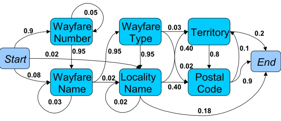
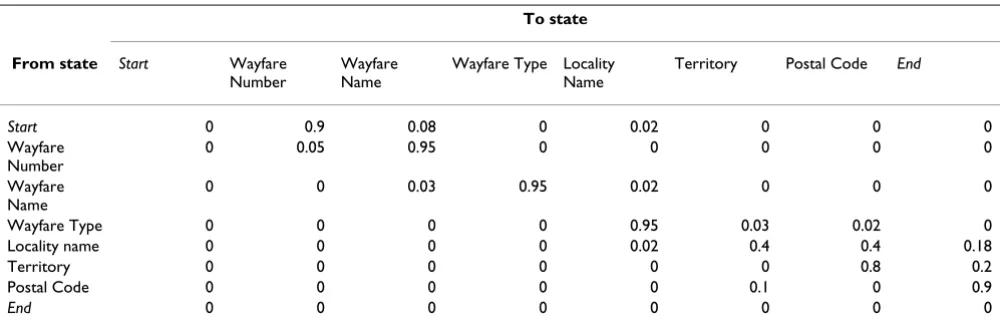
Figure 1 shows a simplified HMM for addresses with eight states. The start and end states are both virtual states as they do not emit any observation symbols. The probabil-ities of transition from one state to another are shown by the arrows (transitions with zero probabilities are omitted for the sake of clarity). The illustrative transition and emission probability matrices for this model are shown in Tables 4 and 5.
Notice that the probabilities in each row of the transition matrix and in each column of the emission matrix add up to one. Also notice that none of the probabilities in the emission matrix are zero. In practice, it is common for some combinations of state and observations symbol not to appear in the training data, resulting in a maximum
likelihood estimate of zero for that element of the emis-sion matrix. Such zero probabilities can cause problems when the model is presented with new data, so smoothing techniques are used to assign small probabilities (in this case 0.01) to all unencountered observation symbols for all states. Traditionally Laplace smoothing is used [26], but Borkar et al. have also described the use of absolute discounting as an alternative when there are a large number of distinct observation symbols [20]. The Febrl
package offers both types of smoothing.
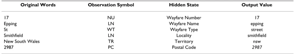
Now consider an example address: "17 Epping St Smith-field New South Wales 2987". This would first be cleaned and tokenised as follows.
['17', 'epping', 'street', 'smithfield', 'nsw', '2987' ]
['NU', 'LN', 'WT', 'LN', 'TR', 'PC' ]
Note that Epping is a suburb of the city of Sydney in the state of New South Wales, Australia, hence the word "ep-ping" in the input string is assigned an LN (locality name) observation symbol even though to a human observer it is clearly a wayfare name in this context. This does not mat-ter because we are ultimately not inmat-terested in the types of the observed symbols but rather in the underlying hidden states which were most likely to have generated them.
Figure 1
Graph of a simplified, illustrative HMM for addresses with eight states Rectangular nodes denote hidden states. Numbers indicate the probabilities of transitions between states, represented by the edges (arrowed lines). Transitions with zero probability are not shown in the interests of clarity.
Start
End
Wayfare
Number
Wayfare
Name
Wayfare
Type
Locality
Name
Territory
Postal
Code
0.9
0.08
0.02
0.05
0.03
0.02
0.95
0.95
0.03
0.02
0.40
0.02
0.40
0.18
0.8
0.2
Even in this very simple model there are 86 = 262,144
pos-sible combinations of hidden states which could have generated this observed sequence of symbols – such as the following sequence of states (with the corresponding ob-servation symbols in brackets):
Start -> Wayfare Name (NU) -> Locality Name (LN) -> Postal Code (WT) > Territory (LN) > Postal Code (TR) -> Territory (PC) -->End
Common sense tells us that this sequence of hidden states is a very unlikely explanation for the observed symbols. From our HMM, the probability of this sequence is indeed rather small (emission probabilities are underlined):
0.08 × 0.01 × 0.02 × 0.8 × 0.4 × 0.01 × 0.1 × 0.01 × 0.8 × 0.01 × 0.1 × 0.01 × 0.2 = 8.19 × 10⁻¹⁷
The following sequence of hidden states is a more plausi-ble explanation for the observed symbols:
Start -> Wayfare Number (NU) -> Wayfare Name (LN) -> Wayfare Type (WT) -> Locality (LN) -> Territory (TR) -> Postal Code (PC) ->End
In fact, according to our simple HMM, this sequence has the greatest probability of all 262,144 possible combina-tions of hidden states and observation symbols and is therefore the most likely explanation for the input se-quence of observation symbols:
0.9 × 0.9 × 0.95 × 0.1 × 0.95 × 0.92 × 0.95 × 0.8 × 0.4 × 0.94 × 0.8 × 0.85 × 0.9 = 1.18 × 10⁻²
It is then a simple matter to use this information to seg-ment the cleaned version of the input string into address elements and output them, as shown in Table 6.
Table 4: Transition probability matrix for simplified, illustrative model
To state
From state Start Wayfare Number
Wayfare Name
Wayfare Type Locality Name
Territory Postal Code End
Start 0 0.9 0.08 0 0.02 0 0 0
Wayfare Number
0 0.05 0.95 0 0 0 0 0
Wayfare Name
0 0 0.03 0.95 0.02 0 0 0
Wayfare Type 0 0 0 0 0.95 0.03 0.02 0
Locality name 0 0 0 0 0.02 0.4 0.4 0.18
Territory 0 0 0 0 0 0 0.8 0.2
Postal Code 0 0 0 0 0 0.1 0 0.9
End 0 0 0 0 0 0 0 0
Table cells contain probabilities of transition from the state listed at the left of each row to the state identified at the top of each column.
Table 5: Emission probability matrix for a simplified, illustrative model
State
Observation Symbol
Start Wayfare
Number
Wayfare Name
Wayfare Type Locality Name
Territory Postal Code End
NU - 0.9 0.01 0.01 0.01 0.01 0.1
-WN - 0.01 0.5 0.01 0.1 0.01 0.01
-WT - 0.01 0.01 0.92 0.01 0.01 0.01
-LN - 0.01 0.1 0.01 0.8 0.01 0.01
-TR - 0.01 0.07 0.01 0.01 0.94 0.01
-PC - 0.04 0.01 0.01 0.01 0.01 0.85
-UN - 0.02 0.31 0.03 0.06 0.01 0.01
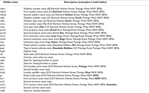
Further details of the way in which HMMs are implement-ed in the Febrl package are available in the associated doc-umentation [22]. The hidden states used in the name and address HMMs are shown in Tables 7 and 8 respectively. These hidden states, and the observation symbols listed Table 3, were derived heuristically from AutoStan tokens and rules developed previously by two of the authors (TC and KL) for use with Australian names and residential ad-dresses. Figures 2 and 3 show directed graphs of these models. Currently, the observation symbols and hidden states are "hard coded" into the Febrl software package, al-though they can be altered by editing the freely available source code. Future versions of the package will use "soft-coded" observation symbols and hidden states, allowing users in other countries to adapt the HMMs for other types of name and address information, or indeed for quite dif-ferent information extraction tasks, without the need for Python programming skills.
Methods
We evaluated the performance of the approach described above with typical Australian residential address data us-ing two data sources.
The first source was a set of approximately 1 million ad-dresses taken from uncorrected electronic copies of death certificates as completed by medical practitioners and cor-oners in the state of New South Wales (NSW) in the years 1988 to 2002. The majority of these data were entered from hand-written death certificate forms. The informa-tion systems into which the data were entered underwent a number of changes during this period.
The second data set was a random sample of 1,000 records of residential addresses drawn from the NSW Inpatient Statistics Collection for the years 1993 to 2001 [27]. This collection contains abstracts for every admission to a pub-lic- or private-sector acute care hospital in NSW. Most of the data were extracted from a variety of computerised hospital information systems, with a small proportion en-tered from paper forms.
Accuracy measurements for name standardisation were conducted using a subset of the NSW Midwives Data Col-lection (MDC) [28]. This subset contained 962,776 records for women who had given birth in New South Wales, Australia, over a ten year period (1990–2000). Most of these data was entered from hand-written forms, although some of the data for the latter years were extract-ed directly from computerisextract-ed obstetric information sys-tems.
Access to these data sets for the purpose of this project was approved by the Australian National University Human Research Ethics Committee and by the relevant data cus-todians within the NSW Department of Health. The data sets used in this project were held on secure computing fa-cilities at the Australian National University and the NSW Department of Health head offices. In order to minimise the invasion of privacy which is necessarily associated with almost all research use of identified data, the medical and health status details were removed from the files used in this project. Thus, for this project the investigators had access to files of names and addresses, but not to any of the medical or other details for the individuals identified in those files, other than the fact that they had died or had given birth.
Address standardisation
Training of HMMs for residential address standardisation was performed by a process of iterative refinement.
An initial hidden Markov model (HMM) was trained us-ing 100 randomly selected death certificate (DC) records. Annotating these records with state and observation sym-bol information took less than one person-hour. The re-sulting model was used to process 1,100 randomly chosen DC records. These records then became a second-stage training set, with each record already annotated with states and observation symbols derived from the initial model. This annotation was manually checked and cor-rected where necessary, which took about 5 person-hours. An HMM derived from this second training set was then used to standardise 50,000 randomly chosen DC records,
Table 6: Example address elements output by a simplified, illustrative model
Original Words Observation Symbol Hidden State Output Value
17 NU Wayfare Number 17
Epping LN Wayfare Name epping
St WT Wayfare Type street
Smithfield LN Locality smithfield
New South Wales TR Territory nsw
and records with unusual patterns of observation symbols (with a frequency of six or less) were examined, corrected and added to the training set if the results produced by the second-stage HMM were incorrect. A new HMM was then derived from this augmented training set and the process repeated a further three times, resulting in the addition of approximately 250 "atypical" training records (bringing the total number of training records to 1,450). The HMM which emerged from this process, designated HMM1, was
used to standardise 1,000 randomly chosen DC test records and the accuracy of the standardisation was as-sessed. Laplace smoothing used in this and all subsequent address standardisation evaluations. Approximately ten hour person-hours of training time was required to reach this point.
HMM1 was then used to standardise 1,000 randomly cho-sen Inpatient Statistics Collection (ISC) test records, and
Figure 2
Graph of the name standardisation HMM evaluated in this study Rectangular nodes denote hidden states. Numbers indicate the probabilities of transitions between states, represented by the edges (arrowed lines). States which were not used and transitions which had a zero probability in the evaluation have been suppressed in the interests of clarity. Prepared with the Graphviz tool http://www.research.att.com/sw/tools/graphviz/.
Start
Given Name 1
0.996
Prefix 1
0.004
Given Name 2
0.104104
Given Name
Hyphen
0.01001
Alt Given
Name 1
0.01001
Surname 1
0.871872
0.004004
0.017094
0.008547
0.957265
0.017094
1.0
1.0
Surname 2
0.222222
Surname
Hyphen
0.777778
1.0
0.3
Table 7: Hidden states for name standardisation currently supported by the Febrl package
Hidden State Description
titl Title (Mr, Ms, Dr etc) state
baby State for baby of, son of or daughter of
knwn State for known as
andor State for and or or
gname1 First given name state
gname2 Second given name state
ghyph Given name hyphen state
gopbr Given name opening bracket or quote state
gclbr Given name closing bracket or quote state
agname1 First alternative given name state
agname2 Second alternative given name state
coma State for commas, semi-colons etc
sname1 First surname state
sname2 Second surname state
shyph Surname hyphen state
sopbr Surname opening bracket or quote state
sclbr Surname closing bracket or quote state
asname1 First alternative surname state
asname2 Second alternative surname state
pref1 First name prefix state
pref2 Second name prefix state
rubb State for residual elements
Table 8: Hidden states for address standardisation currently supported by the Febrl package
Hidden state Description (examples in bold italics)
wfnu Wayfare number state (23 Sherlock Holmes Street, Potingu West NSW 2876) wfna1 First wayfare name state (23 Sherlock Holmes Street, Potingu West NSW 2876) wfna2 Second wayfare name state (23 Sherlock Holmes Street, Potingu West NSW 2876) wfql Wayfare qualifier state (23 Sherlock Holmes Street South, Potingu West NSW 2876) wfty Wayfare type state (23 Sherlock Holmes Street, Potingu West NSW 2876)
unnu Unit number state (Flat 5 23 Sherlock Holmes Street, Potingu West NSW 2876) unty Unit type state (Flat 5 23 Sherlock Holmes Street, Potingu West NSW 2876) prna1 First property name state (Emoh Ruo, Patonga Road, Potingu West NSW 2876) prna2 Second property name state (Emoh Ruo, Patonga Road, Potingu West NSW 2876) inna1 First institution name state (Lost Dogs Home, Patonga Road, Potingu West NSW 2876) inna2 Second institution name state (Lost Dogs Home, Patonga Road, Potingu West NSW 2876) inty Institution type (Lost Dogs Home, Patonga Road, Potingu West NSW 2876)
panu Postal address number state (Roadside Mailbox 234, Patonga Road, Potingu West NSW 2876) paty Type of postal address state (Roadside Mailbox 234, Patonga Road, Potingu West NSW 2876)
hyph Hyphen state
sla Slash state (5/23 Sherlock Holmes Street, Potingu West NSW 2876) coma Comma, semi-colon etc state
opbr State for opening bracket or quote clbr State for closing bracket or quote
loc1 First locality name state (5/23 Sherlock Holmes Street, Potingu West NSW 2876) loc2 Second locality name state
locql Locality qualifier state (5/23 Sherlock Holmes Street, Potingu West NSW 2876) pc Postal code state (5/23 Sherlock Holmes Street, Potingu West NSW 2876) ter1 First territory name state (5/23 Sherlock Holmes Street, Potingu West NSW 2876) ter2 Second territory name state
cntr1 First country name state (5/23 Sherlock Holmes Street, Potingu West NSW 2876, Australia) cntr2 Second country name state
the accuracy assessed. In other words, an HMM trained us-ing one data source (DC) was used to standardise address-es from a different data source (ISC) without any retraining of the HMM.
An additional 1,000 randomly chosen address training records derived from the Midwives Data Collection (MDC) were then added to the 1,450 training records scribed above, and this larger training set was used to de-rive HMM2. HMM2 was then used to re-standardise the
same sets of randomly chosen test records described in the first and second steps above, and the results were assessed.
A further 60 training records, based on archetypes of those records which were incorrectly standardised in all of the preceding tests, were then added to the training set to pro-duce HMM3. HMM3 was then used to re-standardise the same DC and ISC test sets. Thus, HMM3 could be consid-ered as an "overfitted" model for the particular records in the two test sets, although in practice researchers are likely to use such overfitting to maximise standardisation
accu-Figure 3
Graph of the address standardisation HMM evaluated in this study Rectangular nodes denote hidden states. Numbers indicate the probabilities of transitions between states, represented by the edges (arrowed lines). States which were not used and transitions which had a zero probability in the evaluation have been suppressed in the interests of clarity. Prepared with the Graphviz tool http://www.research.att.com/sw/tools/graphviz/.
racy for the particular data sets used in their studies. The total training time for all address standardisation models was not more than 20 person hours.
Finally, by way of comparison, the same two 1,000 record test data sets were standardised using AutoStan in conjunc-tion with a rule set which had been developed and refined by two of the investigators (TC and KL) over several years for use with ISC (but not DC) address data, representing a cumulative investment of at least several person-weeks of programming time.
Name standardisation
To assess the accuracy of name standardisation, a subset of 10,000 records with non-empty name components was selected from the MDC data set (approximately a one per cent sample). This sample was split into ten test sets each containing 1,000 records. A ten-fold cross validation study was performed, with each of the folds having a training set of 9,000 records and the remaining 1,000 records being the test set. The training records were marked up with state and observation symbol informa-tion in about 10 person-hours using the iterative refine-ment method described above. HMMs were then trained without smoothing, and with Laplace and absolute dis-count smoothing, resulting in 30 different HMMs. We found that smoothing had a negligible effect on perform-ance, and only the results from the unsmoothed HMMs are reported here.
The performance of HMMs for name standardisation was compared with a deterministic rule-based standardisation algorithm which is also implemented in the Febrl package – details of this algorithm can be found in the associated documentation [22].
Evaluation criteria
For all tests, records were judged to be accurately stand-ardised when all of the elements present in the input ad-dress string, with the exception of punctuation, were allocated to the correct output field, and the values in each output field were correctly transformed to their canonical form where required. Thus, a record was judged to have been incorrectly standardised if any element of the input string was not allocated to an output field, or if any ele-ment was allocated to the wrong output field. Due to re-source constraints, the investigators were not blind to the nature of the standardisation process (HMM versus Auto-Stan) used. Exact binomial 95 per cent confidence limits for the proportion of correctly standardised records were calculated using the method given in [29].
In the records which were standardised incorrectly, not every data element was assigned to the wrong output field. For each of these address records, the proportions (and
corresponding 95 per cent confidence limits) of data ele-ments which were assigned to the wrong output field, or which were not assigned to an output field at all, were cal-culated. These quantities were not calculated for names due to the much simpler form of the name data.
Computational performance
Indicative run times for the training and application of the HMMs described above were recorded on two computing platforms. Name standardisation was run on a lightly-loaded Sun Enterprise 450 computer with four 480 MHz Ultra-SPARC II processors and 4 gigabytes of main mem-ory, running the Sun Solaris (64-bit Unix) operating sys-tem. Address standardisation was performed on a single-user 1.5 GHz Pentium 4 personal computer with 512 MB of main memory, running the 32-bit Microsoft Windows 2000 operating system. Python version 2.2 was used in both cases. Times were averaged over ten runs.
Results
Addresses standardisation
Results are shown in Table 9.
The mean proportions of data items in each address which were assigned to the incorrect output field, or which were not assigned to any output field, are shown in Table 10.
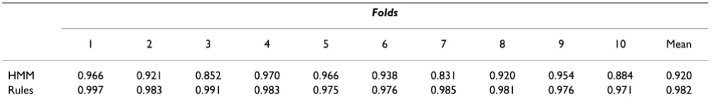
Name standardisation
Results of the ten-fold cross-validation of name standard-isation on 1,000 names of mothers are shown in Table 11.
Computational performance
In all cases it took under 15 seconds to train the various HMMs, once the training data files had been prepared (as described earlier).
HMM standardisation of 103, 104 and 105 name records
on the Sun platform took an average of 67 seconds, 525 seconds and 5133 seconds (86 minutes) respectively, in-dicating that performance scales as O(n) – that is, linearly with the number of records to be processed. HMM stand-ardisation of one million address records on the PC plat-form took 14,061 seconds (234 minutes), or 5832 seconds (97 minutes) with the Psyco just-in-time Python compiler enabled [30]. AutoStan took 1849 seconds (31 minutes) to standardise the same one million address records on the same computer.
Discussion
Address standardisation
sys-tem's rules were developed, and better when used on a dif-ferent data set. In other words, HMMs trained on a particular data source appear to be more general than a rule-based system using rules developed for the same da-ta.
In addition, the improvements in performance observed with HMM2 and HMM3 suggest that, although frequency-based maximum likelihood estimates are used to derive the probability matrices, the resulting HMMs are fairly in-different to the source of their training data, and their per-formance can even be improved by the addition of a small number of "atypical" training records which do not "fit" the HMM very well.
It is probable that some of the observed generality of the HMMs stems from the use of lexicon-based tokenisation as implemented in the Febrl package, which enables ex-haustive but readily available place name and other lists to be leveraged. In contrast, Borkar et al. [20] replaced
each word in each input addresses with symbols based on a simple rational expression grouping eg 3-digit number, 5-digit number, single character, multi-character word, mixed alphanumeric word. These symbols contain much less semantic information than the lexicon-based symbols used in Febrl, although they have the advantage of not re-quiring look-up tables (lexicons). Borkar et al. also used nested HMMs to achieve acceptable accuracy on more complex addresses [20]. At least for Australian addresses, which are of similar complexity to North American ad-dresses, but less complex than most European and Asian addresses, we have not found nested models to be neces-sary. This may be because the lexicon-based tokenisation used in Febrl preserves more information from the source string for use by the HMM, at the expense of a more com-plex model. However, the computational performance of these models is satisfactory. Future attempts at optimisa-tion, by re-writing parts of the code, such as the Viterbi al-gorithm, in C are expected to yield significant increases in speed. In addition, the standardisation of each record is
Table 9: Results of the address standardisation evaluation
HMM/Method
Test Data Set (1000 records) HMM1 HMM2 HMM3 AutoStan
Death Certificates 0.957 (0.943 – 0.969) 0.968 (0.955 – 0.978) 0.976 (0.964 – 0.985) 0.915 (0.896 – 0.932)
Inpatient Statistics Collection 0.957 (0.943 – 0.969) 0.959 (0.945 – 0.970) 0.974 (0.962 – 0.983) 0.953 (0.938 – 0.965)
Table cells contain the proportion of correctly standardised address records for each of the two data sources listed. Ninety-five per cent confidence limits for the proportions are given in brackets.
Table 10: Mean proportion of data items in each address which were assigned to the incorrect output field
HMM/Method
HMM1 HMM2 HMM3 AutoStan
Death Certificates 0.31 (0.25 – 0.37) 0.31 (0.24 – 0.38) 0.33 (0.23 – 0.42) 0.29 (0.26 – 0.32)
Inpatient Statistics Collection 0.23 (0.18 – 0.28) 0.23 (0.18 – 0.28) 0.21 (0.15 – 0.26) 0.19 (0.17 – 0.22)
Table cells contain the mean proportion of data items in each address which were assigned to the incorrect output field, or to no output field. Ninety-five per cent confidence limits for the proportions are given in brackets.
Table 11: Results of name standardisation evaluation
Folds
1 2 3 4 5 6 7 8 9 10 Mean
HMM 0.966 0.921 0.852 0.970 0.966 0.938 0.831 0.920 0.954 0.884 0.920
completely independent from other records, and hence can readily be performed in parallel on clusters of work-stations (COWs).
Standardisation is not an all-or-nothing transformation, and both the rule-based and HMM approaches appear to degrade gracefully when the model or rules make errors. In the address records which were not accurately standard-ised by the HMMs, at least two-thirds of all data elements present in the input record were allocated to the correct output fields. Thus, even these incorrectly standardised records would have considerable discriminatory power when used for record linkage purposes. In only two test records (out of 2000) were all of the address elements wrongly assigned, and both of these were foreign address-es in non-English speaking countriaddress-es. The performance of our AutoStan rule set was similar in this respect.
A significant proportion of incorrectly standardised ad-dresses were of the form "Penryth Downs St Blackstump NSW 2987", which, in the absence of additional informa-tion, could be interpreted as either of the following se-quences of states:
Property Name(UN) -> Wayfare Name(UN) -> Wayfare Type(WT) -> Locality Name(LN) -> Territory(TR) -> Postal Code(PC)
Wayfare Name 1(UN)-> Wayfare Name 2(UN) -> Wayfare Type(WT) -> Locality Name(LN) -> Territory(TR) -> Postal Code(PC)
It is unlikely that further training would assist the HMM in resolving this conundrum. One solution would be to validate the wayfare names as output by the HMM for each locality (where lists of wayfare names for each local-ity are available), and in cases in which the validation fails, to re-allocate the first of the two (apparent) wayfare names as a property name. Other incorrectly standardised records would also benefit from this type of specific post-processing which would be applied only to those records which have been assigned a particular sequence of hidden states by the HMM.
Name standardisation
The performance of the HMM approach for name stand-ardisation, compared to a rule-based approach, was less favourable. Given the simple form of most names in the test data, the rule-based approach was very accurate, achieving 97 per cent accuracy or better, whereas up to 17 per cent of names in the test data were incorrectly stand-ardised by the HMM.
A possible reason for this poor performance may lie in the relative homogeneity of the MDC name data. Out of the
10,000 randomly selected names, approximately 85 per cent were of the simple form "givenname surname", and a further nine per cent were either of the form "givenname gi-venname surname" or "givenname surname surname". Thus the trained HMMs had very few non-zero transition prob-abilities, with a consequent restriction in the number of likely paths through the models.
Names with either two given names or two surnames seemed to be especially problematic. Often the HMMs misclassified the middle name as a second given name in-stead of the first of two surnames. This is due to the large number of names of the form "givenname surname", which resulted in a very high transition probability from the first given name state to the first surname state. Therefore a sec-ond given name is often assigned by the HMM as a first surname, and the real surname as a second surname.
We plan to investigate whether higher-order HMMs, in which the transition probabilities between the current state and a sequence of two or more subsequent states are modelled, may perform better on this type of data.
Other areas which warrant further investigation include the utility of iterative re-estimation of the HMM parame-ters using the Baum-Welch [24], expectation maximisa-tion (EM) [31] or gradient methods [32], and the substitution of maximum entropy Markov models [33] for the hidden Markov models currently used.
One further difficulty is that the estimated probability for the most likely path through the model for each input string depends on the number of words in that string – the more words there are, the more state transitions and hence the lower the overall probability of paths through the model. Thus, input strings cannot be ranked by the maximum probability returned by the Viterbi algorithm in order to find those for which the model is a "poor fit". This problem can be overcome by calculating the "log odds score" [34,35], which is the logarithm of the ratio of the probability that an input string was generated by the HMM to the probability that it was generated by a very general "null" model. Input strings can be ranked by this score, and strings with low scores considered for addition to the training data set.
Conclusions
re-quire substantial initial and ongoing input by skilled programmers in order to set up and maintain complex sets of rules. Instead, clerical staff can be used to create and update the training files from which the probabilistic models are derived.
Future work on the standardisation aspects of the Febrl
package will focus on internationalisation, the addition of post-processing rules which are associated with particular hidden state sequences which are known to be problem-atic, and investigation of higher order models and re-esti-mation procedures as noted above. We hope that other researchers will take advantage the free, open source li-cense under which the package is available to contribute to this development work.
Competing interests
None.
Authors' contributions
TC and PC jointly designed, programmed and document-ed the describdocument-ed software. TC draftdocument-ed the manuscript and PC and KL helped to edit it. TC, PC, KL and JXZ tested the software. KL and TC prepared the evaluation data and the
AutoStan address standardisation rules. TC undertook the evaluation of address standardisation. PC undertook the evaluation of name standardisation. JXZ identified the po-tential utility of HMMs for name and address standardisa-tion and assisted in the documentastandardisa-tion of the software package.
All authors read and approved the final manuscript.
Acknowledgements
This work was equally funded by the Australian National University (ANU) and the New South Wales Department of Health under ANU-Industry Collaboration Scheme (AICS) grant number 1-2001. The authors thank the reviewers for their detailed and helpful comments, which motivated sub-stantial improvements to the paper.
References
1. Gill L, Goldacre M, Simmons H, Bettley G and Griffith M Computer-ised linking of medical records: methodological guidelines.J Epidemiol Community Health 1993, 47:316-319
2. Roos LL and Nicol JP A research registry: uses, development, and accuracy.J Clin Epidemiol 1999, 52(1):39-47
3. Ellsworth DL, Hallman DM and Boerwinkle E Impact of the Hu-man Genome Project on Epidemiologic Research.Epidemiol Rev 1997, 19(1):3-13
4. Khoury MJ Human genome epidemiology: translating advanc-es in human genetics into population-based data for medi-cine and public health.Genet Med 1999, 1(3):71-73
5. Cook LJ, Knight S, Olson LM, Nechodom PJ and Dean JM Motor ve-hicle crash characteristics and medical outcomes among older drivers in Utah, 1992–1995. Ann Emerg Med 2000,
35(6):585-591
6. National Center for Biotechnology Information PubMed Over-view.Bethesda, MA, U.S. National Library of Medicine 2002,
7. Winkler WE Record Linkage Software and Methods for Merg-ing Administrative Lists.Statistical Research Report Series No. RR/ 2001/03, Washington DC, US Bureau of the Census 2001,
8. Gill L Methods for Automatic Record Matching and Linking and their use in National Statistics.National Statistics Methodolog-ical Series No. 25, London, National Statistics 2001,
9. Rahm E and Do HH Problems and Current Approaches.IEEE Bulletin of the Technical Committee on Data Engineering 2000, 23(4):
10. MatchWare Technologies AutoStan and AutoMatch User's ManualsKennebunk, Maine 1998, These products have been sub-sumed into a suite of data quality solutions offered by Ascential Soft-ware Inc. http://www.ascentialsoftSoft-ware.com
11. Soderland S Learning information extraction rules for semi-structured and free text.Machine Learning 1999, 34:233-272 12. Aldelberg B Nodose: a tool for semi-automatically extracting
structured and semistructured data from text documents.In: Proceedings of ACM SIGMOD International Conference on Management of Data New York, Association for Computing Machinery 1998, 283-294 13. Califf ME and Mooney RJ Relational learning of pattern-match
rules for information extraction.In: Proceedings of the Sixteenth National Conference on Artificial Intelligence (AAAI-99), Menlo Park, CA, American Association for Artificial Intelligence 1999, 328-334
14. Rabiner L and Juang B-H Fundamentals of speech recognition.
New Jersey, Prentice-Hall 1993, Ch 6:
15. Bikel DM, Miller S, Schwartz R and Weischedel R Nymble: a high-performance learning name-finder.In: Proceedings of ANLP-97, Haverfordwest, Wales, UK, Association for Neuro-Linguistic Programming
1997, 194-201
16. Freitag D and McCallum A Information extraction using HMMs and shrinkage.In: Papers from the AAAI-99 Workshop on Machine Learning for Information Extraction, Menlo Park, CA, American Association for Artificial Intelligence 1999, 31-36
17. Leek TR Information extraction using hidden Markov models (Master's thesis).University of California San Diego 1997,
18. Freitag D and McCallum A Information extraction with HMM structures learned by stochastic optimisation.In: Proceedings of the Eighteenth Conference on Artificial Intelligence (AAAI-2000), Menlo Park, CA, American Association for Artificial Intelligence 2000, 584-589 19. Seymore K, McCallum A and Rosenfeld R Learning hidden Markov
model structure for information extraction.In: Papers from the AAAI-99 Workshop on Machine Learning for Information Extraction 1999, 37-42
20. Borkar V, Deshmukh K and Sarawagi S Automatic segmentation of text into structured records.In: Electronic Proceedings of ACM SIGMOD Conference 2001: Santa Barbara, California, USA. New York, As-sociation for Computing Machinery 2001,
21. Carnall D Medical software's free future.BMJ 2000, 321:976 22. Christen P and Churches T Joint Computer Science Technical
Report TR-CS-02-05: Febrl – Freely extensible biomedical record linkage.Canberra: Australian National University 2002, 23. van Rossum G and Drake FL Python Reference Manual.Virginia,
PythonLabs Inc. 2001,
24. Rabiner LR A Tutorial on Hidden Markov Models and Selected Applications in Speech Recognition.Proceedings of the IEEE 1989,
77(2):257-286
25. Forney GD The Viterbi Algorithm.Proceedings of the IEEE 1973,
61:268-278
26. Laplace P-S Nine Philosophical Essays on Probabilities. (Trans-lated by A.I. Dale from the 5th French edition of 1825), New York, Springer
1995,
27. New South Wales Department of Health NSW Health Data Col-lections – Inpatient Statistics Collection.Sydney 2002, 28. Public Health Division New South Wales Mothers and Babies
2000.N S W Public Health Bull 2001, 12(S-3):1-114
29. Armitage P, Berry G and Matthews JNS Statistical Methods in Medical Research.Oxford, Blackwell Science 2002, 117
30. Rigo A Psyco: the Python specialising compiler.Brussels: Univer-sité Libre de Bruxelles 2002,
31. Dempster AP, Laird NM and Rubin DB Maximum likelihood from incomplete data via the EM algorithm.J Roy Stat Soc 1977,
39(1):1-38
32. Levinson SE, Rabiner LR and Sondhi MM An introduction to the application of the theory of probabilistic functions of a Mark-ov process to automatic speech recognition.Bell Systems Tech-nical Journal 1983, 62(4):1035-1074
Publish with BioMed Central and every scientist can read your work free of charge
"BioMed Central will be the most significant development for disseminating the results of biomedical researc h in our lifetime."
Sir Paul Nurse, Cancer Research UK
Your research papers will be:
available free of charge to the entire biomedical community
peer reviewed and published immediately upon acceptance
cited in PubMed and archived on PubMed Central
yours — you keep the copyright
Submit your manuscript here:
http://www.biomedcentral.com/info/publishing_adv.asp
BioMedcentral 34. Altschul SF Amino acid substitution matrices from an
infor-mation theoretic perspective.JMB 1991, 219:555-565 35. Barrett C, Hughey R and Karplus K Scoring hidden Markov
mod-els.Comput Appl Biosci 1997, 13(2):191-199
Pre-publication history
The pre-publication history for this paper can be accessed here: