Analysis of animal accelerometer data using hidden Markov models

Short running title: Hidden Markov models for accelerometer data

Analysis of animal accelerometer data using hidden Markov

models

Vianey Leos-Barajas

, Theoni Photopoulou

, Roland Langrock

, Toby A. Patterson

,

Yuuki Y. Watanabe

_{, Megan Murgatroyd}

_{and Yannis P. Papastamatiou}

a

_{Department of Statistics}

Iowa State University

Ames, IA, USA

b

_{Centre for Statistics in Ecology, Environment and Conservation}

Department of Statistical Sciences

University of Cape Town

Cape Town, South Africa

c

_{Department of Business Administration and Economics}

Bielefeld University

Bielefeld, Germany

d

_{CSIRO, Oceans and Atmosphere}

Hobart, Tasmania, Australia

e

_{National Institute of Polar Research}

Tachikawa, Tokyo, Japan

f

_{SOKENDAI (The Graduate University for Advanced Studies)}

Tachikawa, Tokyo, Japan

g

_{Animal Demography Unit}

University of Cape Town

Cape Town, South Africa

h

_{School of Biology, Scottish Oceans Institute}

University of St Andrews

St Andrews, UK

i

_{Department of Biological Sciences}

Florida International University

North Miami, Fl, USA

Word Count: –

∗_{corresponding author:}

e-mail: [email protected]

Abstract

1

1. Use of accelerometers is now widespread within animal biotelemetry as they provide a means 2

of measuring an animal’s activity in a meaningful and quantitative way where direct observation is 3

not possible. In sequential acceleration data there is a natural dependence between observations of 4

behaviour, a fact that has been largely ignored in most analyses. 5

2. Analyses of acceleration data where serial dependence has been explicitly modelled have largely 6

relied on hidden Markov models (HMMs). Depending on the aim of an analysis, an HMM can be 7

used for state prediction or to make inferences about drivers of behaviour. For state prediction, 8

a supervised learning approach can be applied. That is, an HMM is trained to classify unlabelled 9

acceleration data into a finite set of pre-specified categories. An unsupervised learning approach can 10

be used to infer new aspects of animal behaviour when biologically meaningful response variables 11

are used, with the caveat that the states may not map to specific behaviours. 12

3. We will provide the details necessary to implement and assess an HMM in both the supervised 13

and unsupervised learning context and discuss the data requirements of each case. We outline 14

two applications to marine and aerial systems (shark and eagle) taking the unsupervised learning 15

approach, which is more readily applicable to animal activity measured in the field. HMMs were 16

used to infer the effects of temporal, atmospheric and tidal inputs on animal behaviour. 17

4. Animal accelerometer data allow ecologists to identify important correlates and drivers of animal 18

activity (and hence behaviour). The HMM framework is well suited to deal with the main features 19

commonly observed in accelerometer data, and can easily be extended to suit a wide range of types 20

of animal activity data. The ability to combine direct observations of animal activity with statistical 21

models, which account for the features of accelerometer data, offers a new way to quantify animal 22

behaviour, energetic expenditure and deepen our insights into individual behaviour as a constituent 23

of populations and ecosystems. 24

Keywords: animal behaviour; activity recognition; latent states; serial correlation; time series 25

1

Introduction

26

Accelerometers are becoming more prevalent in the fields of animal and human bio-logging (Bao & 27

Intille, 2004; Raviet al., 2005; Shepardet al., 2008; Altunet al., 2010). The potential of accelerometers 28

lies in the fact that they provide a means of measuring activity in a meaningful and quantitative way 29

where direct observation is not possible (Shepardet al., 2008; Nathanet al., 2012; Brownet al., 2013). 30

While these instruments are cheap and compact, recording acceleration at a high temporal resolution and 31

in up to three dimensions quickly results in terabytes of data that present various challenges regarding 32

transmission, storage, processing and statistical modelling. 33

Much of the focus in the analysis of acceleration data has been on identifying patterns in the 34

observed waveforms that correspond to a known behaviour or movement mode. This can be achieved 35

by employing statistical classification methods and can entail observing the animal, manually assigning 36

data in order to subsequently classify remaining unlabelled data. Many studies that have shown the 38

effectiveness of various machine learning algorithms for classification of human acceleration data (Bao & 39

Intille, 2004; Raviet al., 2005; Altunet al., 2010; Mannini & Sabatini, 2010). Algorithms such as support 40

vector machines (SVM), classification trees, random forests, among others, have also recently been used 41

for classification of animal acceleration data (Nathanet al., 2012; Carrollet al., 2014; Grafet al., 2015). 42

For example, Nathan et al. (2012) compared the effectiveness of five machine learning algorithms to 43

distinguish between eating, running, standing, active flight, passive flight, general preening and lying 44

down, for griffon vultures. 45

Most machine learning algorithms assume independence between individual observations. However, 46

in sequential acceleration data there is a natural dependence between observations of behaviour — 47

once initiated, particular animal behaviours often last for periods longer than the sampling frequency. 48

This fact has been largely ignored in most applications of classification approaches. The studies where 49

serial dependence has been explicitly modelled have mostly relied on hidden Markov models (HMMs) 50

(Wardet al., 2006; Heet al., 2007; Mannini & Sabatini, 2010, 2011). HMMs are stochastic time series 51

models which assume that the observed time series, the so-called state-dependent process, is driven by 52

an unobservable state process. In this scenario, the former corresponds to the acceleration data and the 53

latter to the behavioural classes. Typically, and in common with the aforementioned machine learning 54

approaches, in the training stage, the states of the HMM were known a priori, requiring corresponding 55

data derived from direct observations. 56

There are two main difficulties with such a supervised learning approach. First, while there has been 57

much success in classification of human acceleration data, where training data can usually be obtained 58

with minimal effort, this may not be feasible for some animals. Humans can easily be observed in a 59

laboratory setting, given instructions or monitored in more realistic settings, such as walking outdoors or 60

in their home (e.g. Leenderset al., 2000). In certain cases, animals can also be monitored in a laboratory 61

setting (Wilsonet al., 2008), but movement patterns recorded in the lab from free-ranging animals may 62

not appear exactly the same as in data collected while in more natural settings. Conversely, many 63

behaviours can only be observed in natural settings, although there has been success using surrogate 64

species for classification of behavioural modes (Shepardet al., 2008; Nathanet al., 2012; Campbellet al., 65

2014; Brownet al., 2013). 66

Second, human acceleration data has commonly been used as a tool for health monitoring and other 67

situations where the focus is on (state) prediction, as opposed to learning how external factors drive 68

the behaviours. Classification of behavioursalone, while certainly of interest in many scenarios, may 69

not lead to biologically interesting inference. Once the classification has been done, the task of relating 70

these states to environmental (and other) covariates in order to identify drivers in behaviours remains. 71

Moreover, it is difficult to make appropriate inferential statements as the classifications are not without 72

error, propagating the state uncertainty through to the modelled effect of the covariates. 73

the HMM to recognize specific behaviours. Alternatively, HMMs can also be used in an unsupervised 75

learning context, i.e. when there are no labelled data. In an unsupervised learning context the states 76

are not pre-defined to represent a specific behaviour. Instead, the states will be allocated such that the 77

model captures as much as possible of the marginal distribution of the observations, i.e. the distribution 78

of an observation at a randomly chosen time point, not conditional on the previous history of the 79

process, as well as their correlation structure. If biologically meaningful response variables from the 80

acceleration data are considered, then the HMM states will usually represent interpretable activity levels 81

or even proxies of behavioural modes. Being data-driven the states can be as, if not more, informative 82

in the unsupervised learning setting than the alternatives. We can then incorporate exogenous or, 83

where available, endogenous variable(s) of interest, to make inferential statements. HMMs and related 84

state-switching models, in particular state-space models, have successfully been implemented to identify 85

drivers of movement based on tracking data (Pattersonet al., 2009), and can similarly be applied in the 86

context of accelerometer data. For example, Phillips et al.(2015) applied HMMs in an unsupervised 87

learning context to understand the behaviour of free swimming tuna from vertical movement data 88

collected by data-storage tags. We will implement an unsupervised learning approach for another 89

difficult to observe marine species, the blacktip reef shark, and a volant species, the black eagle. 90

In this paper we review HMM-based approaches to the analysis of animal accelerometer data. In 91

Section 2 we will provide an overview of accelerometer data and connect the data processing step to the 92

HMM-based approaches described in Section 3. We will typically refer to the termbehavioural class, 93

rather than differentiate between identification of specific movements (e.g. wing flapping) or behaviours 94

(e.g. foraging). In Section 4 we demonstrate the use of HMMs with real data examples from marine 95

and aerial systems. 96

2

Accelerometer data

97

Accelerometer devices measure in up to three axes, which can be described relative to the body of the 98

animal; longitudinal (surge), lateral (sway) and dorso-ventral (heave). Acceleration recorded along one 99

or two axes can be used to measure movement in parts of the body, e.g. the mandible (Suzukiet al., 100

2009; Naitoet al., 2010; Iwata et al., 2015), or aspects of whole body acceleration, e.g. longitudinal 101

surge (Sakamotoet al., 2009). Currently, acceleration is most commonly recorded in three axes and, to 102

a lesser degree, in two axes (Brownet al., 2013), to measure locomotion. 103

104

2.1

Data Processing for Classification

105

While the observed acceleration data can be used to identify specific movements in animals, HMMs and 106

other machine learning algorithms require more information to accurately classify the unlabelled data. 107

of observations. The derived features should be driven by the classes of movements that have been 109

defined and chosen in such a way to accentuate the differences in observed acceleration measurements. 110

There are many commonalities between the features used in applications of classification of accelera-111

tion data, though naturally no one optimal set exists (Bao & Intille, 2004; Martiskainenet al., 2009; 112

Nathanet al., 2012; Brownet al., 2013). For instance, Nathan et al.(2012) used thirty-eight features 113

in order to distinguish between eating, running, standing, active flight, passive flight, general preening 114

and lying down, for griffon vultures, while Grafet al.(2015) used eight features to distinguish between 115

standing, walking, swimming, feeding, diving and grooming of Eurasian beavers. In each case, means 116

and variances of each of the three axes are used, as well as overall dynamic body acceleration (ODBA), 117

the sum of dynamic body acceleration from the three axis, among others. 118

119

2.2

Connecting Measures to Behaviours

120

When the aim is to classify the acceleration data, data processing is driven by identifying a set of features 121

that can be used to distinguish between specific behaviours, even if those features are not themselves 122

interpretable as a specific behaviour when considered on their own. However, there are metrics derived 123

from accelerometer data that, on their own, can be used as proxies for behaviour and as input to an 124

HMM. Repeating patterns in at least one axis tend to arise from behaviours such as stroking (Sakamoto 125

et al., 2009), flapping, running or walking (Shepardet al., 2008), whereas sudden changes, corresponding 126

to bursts of acceleration, are often associated with prey pursuits or capture (Suzukiet al., 2009; Simon 127

et al., 2012; Ydesenet al., 2014; Heerahet al., 2014), as well as predator avoidance or conflict. 128

In addition to behaviour, several measures can be used to summarise effort or exertion and relate 129

acceleration to activity levels, such as ODBA (Wilsonet al., 2006; Gleisset al., 2011; Elliottet al., 2013; 130

Gleisset al., 2013) and vectorial dynamic body acceleration (VeDBA) (Qasem et al., 2012). Minimum 131

specific acceleration (MSA) (Simonet al., 2012) can be used to disentangle the gravitational component 132

of acceleration (static acceleration) from the movement signal or specific acceleration (also dynamic 133

acceleration). One of the simplest and most unambiguous interpretations of static acceleration data is 134

body posture, which in many cases can be directly interpreted as a specific behaviour (Wilsonet al., 135

2008; Shepardet al., 2008). 136

Both ODBA and MSA are used to reduce the dimensionality of 3D acceleration data while retaining 137

important information (e.g. Wilsonet al.(2008); Simonet al.(2012)). They remove the gravitational 138

component from the acceleration signature and produce an overall value of the dynamic acceleration 139

experienced by the animal. ODBA is derived by smoothing over a time period, e.g. 1 sec, making it 140

useful for continuous data, whereas MSA is calculated point-wise (as the norm of the three vectors 141

3

Analysis of accelerometer data

143

We will first provide a brief overview of the HMM framework (Section 3.1). Subsequently, in Section 3.2, 144

we will review how HMMs can be used for state prediction, i.e. classification of animal accelerometer 145

data. In Section 3.3, we focus on the implementation of HMMs in a setting where the meaning of the 146

states is driven entirely by the data and the focus lies on general inference rather than classification 147

only. 148

3.1

Hidden Markov models

149

An HMM is a stochastic time series model involving two layers: an observablestate-dependent process, 150

denoted by{Yt}Tt=1(in the univariate case), and an unobservablestate process, denoted by{Ct}Tt=1. The

151

state-dependent process models the observations, while the state process is a latent factor influencing the 152

distribution of the observations. In our case, the observations are the accelerometer metrics considered, 153

and the latent states are closely related to the animal’s behavioural state. More specifically, the state 154

process{Ct} takes on a finite number of possible values, 1, . . . , M, and its value at timet, ct, selects

155

which ofM possible component distributions generates observationyt. The Markov property is assumed

156

for{Ct}, i.e. the (behavioural) state at time t only depends on the (behavioural) state at timet−1,

157

such that evolution of the process over time is completely characterized by the one-step state transition 158

probabilities. These models are natural and intuitive candidates for modelling animal accelerometer 159

data, for two reasons: 1) they directly account for the fact that any corresponding observation will 160

be driven by the underlying behavioural state, or general activity level, of the animal, and 2) they 161

accommodate serial correlation in the time series by allowing states to be persistent. HMMs seek 162

to capture the strong autocorrelation in accelerometer data in a mechanistic way, rather than either 163

neglecting this feature completely or only including it in a nuisance error term. HMMs can therefore be 164

used for inference on complex temporal patterns, including the behavioural state-switching dynamics 165

and how these are driven by environmental variables (Pattersonet al., 2009; McKellaret al., 2015). 166

To complete the basic HMM formulation, we first summarize the probabilities of transitions between 167

the different states in the M ×M transition probability matrix (t.p.m.) Γ = (γij), where γij =

168

Pr Ct+1 = j|Ct = i

(for any t), i, j = 1, . . . , M. Note that here we are assuming that the state 169

transition probabilities are constant over time; this assumption will be relaxed in Section 3.3. The 170

initial state probabilities are summarized in the row vectorδ, where δi= Pr(C1=i),i= 1, . . . , M.

171

Second, we need to specify state-dependent distributions (sometimes called emission distributions), 172

p(yt|Ct = m), or more succinctly pm(yt), for m = 1, ..., M. These distributions can be discrete or

173

continuous, and possibly also multivariate (in which case we write yt = (y1t, . . . , yRt)). Usually, the

174

same parametric distribution is assigned to all M states, such that each state differs in terms of its 175

associated values of the parameters. Selection is driven by the data itself, e.g. count data or continuous 176

3.2

State prediction

178

HMMs provide a solid framework for the classification of data with strong serial dependence, such as 179

sequential acceleration data, which are often processed to represent movements over a few seconds, or 180

less, at a time (Wardet al., 2006; Heet al., 2007; Mannini & Sabatini, 2010). In this section, we will 181

cover the implementation and testing of an HMM when the focus of the analysis is state prediction. A 182

full example and R code implementing this approach is provided in the Supplementary material. 183

State prediction can be accomplished in three manners, commonly referred to as supervised, semi-184

supervised, or unsupervised learning. We will discuss the implementation of an HMM in the supervised 185

learning case, such that each state will correspond to one behaviour of interest, and briefly comment 186

on the other two cases at the end of the section. Hastie et al. (2001) detail how to split the labelled 187

time series into training, validation, and testing data, in order to estimate the prediction error. Other 188

approaches to estimating prediction error, such as a leave-one-out cross-validation (here treating a time 189

series as an observation), are also provided in detail. 190

Since the states are known, the maximum likelihood estimates (MLEs) of the HMM parameters are 191

obtained by maximizing the complete-data likelihood, which conveniently splits into several independent 192

parts, each of which is fairly straightforward to maximize (details provided in the Appendix). First, the 193

m-th entry of ˆδis simply the proportion of the time series that start in statem. Second, the entries of 194

the t.p.m. are estimated by 195

ˆ

γij =

# transitions from stateito statej

total # transitions from statei ,

196

fori, j = 1, ..., M. (Note this is the MLE conditional on the initial state, c1.) Finally, for each m =

197

1, . . . , M, the parameters of the state-dependent distribution given statemare estimated using only the 198

observations allocated to statem. As a multivariate normal distribution (MVN) is a common choice in 199

these cases, we cover the steps to fit the HMM with MVN state-dependent distributions in the Appendix 200

and Supplementary material. Given a fitted HMM, we can use the Viterbi algorithm to decode the most 201

likely state sequence, thereby assigning each observation to a state, at low computational effort. Full 202

details for state decoding are provided in Zucchiniet al.(2016). The state predictions can be compared 203

to the known states, and the proportion of correctly decoded states serves as an estimate of the prediction 204

accuracy. 205

As mentioned previously, there are two other approaches to state-prediction: semi-supervised and 206

unsupervised learning. In a semi-supervised approach, classes are pre-defined, as in the supervised 207

learning context, but there is additional flexibility provided in that the data do not have to be assigned 208

to one of the pre-defined classes. Instead, multiple additional states can be estimated from the data. In 209

an unsupervised learning approach, classes are not pre-defined in any manner. In these two cases, one 210

objective can be to identify the number of distinct movement patterns exhibited by the animal, with 211

multiple movement modes can correspond to the same behaviour (e.g foraging), interpretation of the 213

estimated states should be made with caution. In the next section, we will detail the implementation 214

of the unsupervised learning approach where the focus is to construct biologically relevant classes of 215

animal behaviour in order to make inferential statements. 216

3.3

Inference

217

So far, we have mostly focused on the case where there is a training sample, i.e. acceleration data together 218

with the associated behavioural states. Corresponding analyses involve training the HMM based on such 219

labelled data and then using that HMM to categorize incoming new, unlabelled data. While certainly of 220

interest in some settings, in practice, more often than not, labelled data will not be available but only the 221

accelerometer data. In such unsupervised learning settings, the HMM framework can be equally useful, 222

but is typically applied for different purposes than in classification. More specifically, the meaning of the 223

states in such cases is often not of interestper se. Instead, an HMM is used simply as an approximate 224

representation of the real data-generating process, and this may or may not entail that the nominal 225

HMM states are biologically meaningful. (However, metrics derived from the accelerometer data, as 226

described in Section 2, have been shown to provide insight into activity levels or correspond to classes 227

of behaviours, such that when used as response variables in the HMM these can lead to biologically 228

interpretable states.) Unsupervised learning of HMMs for accelerometer data has the advantage that 229

the states are estimated in a data-driven manner. In particular, for many of the metrics described in 230

Section 2 that are connected to behaviours, assignment of classes is difficult, to say the least, especially 231

for animals where behaviours are not well-defined. These include animals which cannot be directly 232

observed for long periods such as aquatic organisms. 233

There are three different possible purposes of having an approximate representation of the real pro-234

cess: (i) a mathematical description of the dynamics of the system (e.g. in order to have a concise 235

description of how accelerometer measurements evolve over time, in terms of a small number of in-236

terpretable parameters and associated stochastic distributions); (ii) extraction of information (e.g. a 237

hypothesis test on whether or not some environmental covariate increases the probability of an animal 238

switching to a particular behavioural state); (iii) prediction of future or missing values (e.g. behavioural 239

state prediction given accelerometer data) — see Konishi & Kitagawa (2008). In the ecological litera-240

ture on animal movement modelling, HMMs are used primarily to address (i) and (ii), the former in the 241

sense that concise descriptions of movement patterns are sought, the latter in the sense that inference 242

on the interaction of animals with their environment is drawn. In general, the ability to make inferential 243

statements provides an avenue to answer questions about the behavioural processes, movement patterns 244

and transitions between behaviours under different in relation to covariates. 245

Addressing a research question related to aim (ii) usually involves the incorporation of covariates 246

into the statistical model. In the HMM setting, this is commonly done at the level of the hidden states. 247

probability matrixΓ(t)= (γ(_ijt)), whereγ_ij(t)= Pr(Ct+1=j|Ct=i). The transition probabilities at time

249

t, γ(_ijt), can then be related to a vector of environmental (or other) covariates, ω₁(t), . . . , ω(pt)

, via the 250

multinomial logit link: 251

γ_ij(t)= exp(ηij) PN

k=1exp(ηik)

, where ηij =

  

 

β₀(ij)+Pp

l=1β (ij)

l ω

(t)

l ifi6=j;

0 otherwise.

252

Essentially there is one multinomial logit link specification for each row of the matrix Γ(t)_{, and the}

253

entries on the diagonal of the matrix serve as reference categories. 254

While with labelled data the likelihood of interest is the complete-data likelihood, for unlabelled 255

data the likelihood of interest is the density of the observations only,L=p(y1, . . . ,yT), the evaluation

256

of which requires the consideration of all possible state sequences that might have given rise to these 257

data. The powerful forward algorithm, detailed in the Appendix, can be applied to accomplish this, 258

opening up a straightforward and usually feasible avenue to MLEs, namely direct numerical maximiza-259

tion of the likelihood. In practice, one needs to consider multiple starting values in order to make 260

sure to have found the global maximum. The Expectation-Maximization algorithm provides a popular 261

alternative route to MLEs, despite being much more technically involved and having no clear practical 262

advantages (MacDonald, 2014). Since it is our view that users are better off focusing on the simpler 263

direct maximization approach, it is only this approach that we present in detail in the Appendix and 264

Supplementary material (for a more comprehensive introduction to maximum likelihood estimation for 265

HMMs, see Zucchiniet al., 2016). 266

Model selection techniques, in particular information criteria, can be used to choose an adequate 267

family of state-dependent distributions, to select an appropriate number of states or to determine 268

whether or not a covariate should be included in the model. However, users should not blindly follow 269

such information criteria, especially with regard to the selection of the number of states. For animal 270

behaviour data, it is our experience that such formal model selection approaches tend to favour models 271

with more states than would be expected based on biological intuition, often to an extent such that 272

selected models become near-impossible to interpret and very difficult to work with in practice (Langrock 273

et al., 2015). One explanation for this is that often additional states are included to compensate for a 274

model formulation that ignores some pattern in the data. These patterns can be due to the influence of 275

an unobserved covariate, within-day variation or individual heterogeneity which is not accounted for, a 276

violation of the Markov assumption or outliers — which usually cannot be avoided in data structures 277

as complex as those studied here, and which may not be pertinent to the ultimate aim of the study. 278

Further, accelerometer data is directly connected to the movement of an animal, such that an HMM 279

with a large number of states may reflect multiple movement modes, or general classes of movement, 280

connected to the same behavioural class, e.g. foraging or active behaviour. In such cases a healthy dose 281

of pragmatism is required. If the choice of the number of states turns out to be difficult, then it is often 282

model checking tools, in order to understand what exactly it is that the more complex models capture 284

that is not already captured by the simpler models. Langrocket al. (2015) discuss this issue in detail, 285

demonstrating many of the points made above in a real data example. 286

The HMM framework encompasses various other useful tools for drawing inference. In particular, 287

incorporating random effects into the model formulation will be crucial when there is substantial hetero-288

geneity across multiple individuals observed. There are various ways in which this can be accomplished 289

within the class of HMMs — see McKellar et al. (2015) and Chapter 13 in Zucchiniet al. (2016) for 290

comprehensive overviews, including discussions on the importance of acknowledging any potential het-291

erogeneity. Furthermore, the dependence structure can be modified in various ways, e.g. allowing for 292

more complex memory in the state process without losing the ability to efficiently calculate the likeli-293

hood using the forward algorithm (Langrocket al., 2012). Assessment of the model adequacy, i.e. model 294

checking, is commonly done using (pseudo-)residuals, which can reveal any notable lack of fit (Zucchini 295

et al., 2016). 296

4

Real data examples

297

4.1

Modelling activity in a soaring raptor

298

Large soaring birds, like raptors, depend on favourable meteorological conditions, as well as the un-299

derlying topography, for generation of updrafts required for low-energy flight (Pennycuick, 2008). Lift 300

availability is known to be driven largely by wind speed and temperature, as well as their interaction 301

with the underlying topography, though other factors also contribute. Lift adequate for soaring flight is 302

generated by two mechanisms; (1) by upward thermal convection of air warmed by solar radiation ( ´Akos 303

et al., 2010) (thermal soaring), and (2) by the movement of air over slopes and ridges in the landscape 304

(orographic or ridge soaring). 305

Recently, empirical studies relating bird activity patterns to weather conditions have become pos-306

sible due to advances in bio-logging technology that allows for collection of high-resolution movement 307

(e.g. acceleration) data. In particular, acceleration data can be used to distinguish between different 308

movement modes or, more simply, as a proxy of overall activity level, even if they do not correspond 309

clearly to different behaviours (Williamset al., 2015). 310

An adult Verreaux’s eagle(Aquila verreauxii)was instrumented with a remotely downloadable multi-311

sensor data-logger (UvABiTS, University of Amsterdam, The Netherlands, Boutenet al.(2013)) in the 312

Western Cape, South Africa, in 2013. The data-logger recorded 3D acceleration (at 20 Hz) for 1 second 313

directly after recording GPS location. The GPS location sampling rate depended on the solar-powered 314

battery charge and thus was higher during the mid-day. Data were collected over 9 consecutive days, 315

with a variable amount of acceleration data sampled each day and none collected overnight. 316

We were primarily interested in identifying potential drivers of activity level. As such, we extracted 317

On average, each day produced approximately 135 observations (s.e. 23.32). Before fitting an HMM to 319

the time series of MSA values, we first needed to resolve the irregular sampling of the acceleration data, 320

as this is a clear violation of the HMM assumptions. The time series of MSA across days were taken to 321

be independent and, within a day, the acceleration data was subsampled to produce one value of MSA 322

every 112 seconds. Only 1 consecutive missing value was allowed before splitting the daily MSA time 323

series into two or more segments. 324

The histogram of MSA values revealed two peaks close to zero, which may reflect general low-active 325

behaviours such as roosting and preening. As we did not wish to discriminate between these two general 326

types of behaviours, we fit a 2-state HMM with state 1 represented by a mixture of gamma distributions 327

and a gamma distribution for state 2. The fitted state-dependent densities are shown in Figure 2, which 328

wepost-hoc interpreted as low-activity and high-activity behaviour. Although we do not connect state 329

2 to a specific flight behaviour, such as orographic soaring, we expect that behaviours requiring more 330

energy are reflected by larger MSA values. 331

In order to examine the effect of wind speed and temperature on the state-switching dynamics be-332

tween the two activity levels, we obtained hourly observations from the South African Weather Services 333

(Lambert’s Bay Station). The station is approximately 30 km from the general area in which the eagle 334

was tracked, which lead to a slight spatial and temporal mismatch between the available weather data 335

and the conditions actually experienced by the eagle. The range of temperatures and wind speeds expe-336

rienced by the eagle during the study period was between 12.3–31.5◦C, and 0–7.4 m/sec, respectively. 337

We allowed the entries of the t.p.m. to be a function of up to wind speed, temperature and their inter-338

action. The wind-only model is written as logit(γij(t)) =β0i+β1ix1t, for i= 1,2,j 6=i,t= 1, . . . , T,

339

with the intercept termβ0,i reflecting the t.p.m. when wind speed is at 0 m/sec. The model including

340

wind speed alone was favoured by the Bayesian Information Criterion (BIC) and the full model, with 341

temperature and the interaction term, favoured by the Akaike Information Criterion (AIC) (Table 1). 342

After examination of the (pseudo-)residuals of the models selected by AIC and BIC, we selected the 343

model favoured by BIC as there was a similar lack-of-fit evident in both models. Further, we may 344

not have captured a large enough range of temperatures in order to make general inferences about its 345

effect on the activity levels of the eagle, and as such were cautious of over-fitting or over-interpreting 346

the model results. We present confidence intervals and a plot of the (pseudo-)residuals for assessment 347

of goodness-of-fit in the Appendix for the model with only wind speed included. R code to simulate 348

MSA data and fit a 2-state HMM with the t.p.m. entries as functions of wind speed is included in the 349

Supplementary material. 350

The estimated state transition probabilities suggest that, as wind speed increases, (i) the eagle has a 351

very slightly increased chance of switching to the high-activity state when in the low-activity state, and 352

(ii) spends much longer periods of time, on average, in the active state. As a consequence, the equilibrium 353

(stationary) distribution for fixed wind speeds (Pattersonet al., 2009) indicates that the eagle spends 354

orographic soaring, as demonstrated by studies on migrating golden eaglesAquila chrysaetos, which is 356

a more active behaviour (Lanzone et al., 2012). There is also theoretical evidence to suggest that, in 357

general, flying is more energetically demanding in high winds (Pennycuick, 1972). 358

4.2

Diel activity changes in a reef-associated shark

359

Many species of shark are upper trophic level predators may serve an important role in marine ecosys-360

tems. However determining the intensity of their predatory behaviour requires modelling the temporal 361

component as their activity levels are likely to follow a diel and/or tidal cycle (e.g. Gleisset al., 2013; 362

Papastamatiouet al., 2015). Acceleration sensors provide a direct measure of activity, however, many 363

species of shark swim continuously making it difficult to define specific behaviours (e.g. they are never 364

truly at rest), making conventional classification methods problematic. HMMs can identify changes 365

in behavioural states and how these may be related to time of day, tidal state, swimming depth, or 366

water temperature. To demonstrate this, we applied HMMs to accelerometry data obtained from a 367

free-ranging blacktip reef shark (Carcharhinus melanopterus) at Palmyra Atoll in the central Pacific 368

ocean (data taken from Papastamatiouet al., 2015). A multi-sensor package was attached to the dorsal 369

fin of a 117 cm female shark. The multi-sensor data-logger (ORI400-D3GT, Little Leonardo, Tokyo, 370

Japan) recorded 3D acceleration (at 20 Hz), depth and water temperature (at 1 Hz) and was embedded 371

in a foam float which detached from the shark after four days (see Papastamatiou et al., 2015). The 372

package also contained a VHF transmitter allowing recovery at the surface after detachment. 373

In order to examine active behaviour, we calculated the average ODBA of the shark over 1 second 374

intervals, which resulted in 321,815 observations (after removing the first four hours of data). Figure 375

4 displays the ODBA time series of one day. Compared to metrics such as tail-beat frequency, ODBA 376

has the advantage of measuring change in behaviour in all axes. For example, if the shark is nose down 377

at the seafloor, attempting to capture prey, its tail-beat frequency may be low but it is still active. As 378

we are interested in the times of day the shark was more active, as well as tide effects, we applied a 379

2-state HMM with one statepost-hoc interpreted as representing less active behaviour and the other 380

more active behaviour. 381

Although there are clear spikes in ODBA that point to higher energetic activities, various combi-382

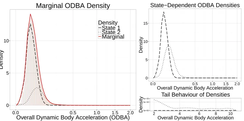
nations of parametric distributions for state 1 and 2 led to vastly different state-dependent densities. 383

Further, the ODBA values had many extreme values that needed to be accommodated, which further in-384

creased the difficulties of selecting appropriate state-dependent distributions. As ODBA is not a metric 385

that can easily be divided into active/inactive behaviours in sharks, we estimated the state-dependent 386

densities nonparametrically, in both states, in order to minimize the bias introduced by assigning inad-387

equate parametric distributions (Langrocket al., 2015). Figure 5 displays the fitted distributions. 388

To examine potential diel and tide effects on activity levels, we let the entries of the t.p.m. be 389

functions of up to two covariates: time of day and tide level (ebb, flood, low, and high). Tide data was 390

high or low tide as±1 hour from reported high or low tide times. Time of day is represented by two 392

trigonometric functions with period 24 hours, cos(2πt/86400) and sin(2πt/86400) (86,400 is the number 393

of seconds in a day). We use three indicator variables,x1t, x2tand x3t, for tide levelshigh,flood, and

394

ebb, respectively, such thatx1t= 1 when tide level is high andx1t= 0 otherwise, and so on, which gives

395

the entries of the t.p.m. the following form 396

logit(γij(t)) =β0i+β1icos(2πt/86400) +β2isin(2πt/86400) +β3ix1t+β4ix2t+β5ix3t

397

fori= 1,2,j6=i,t= 1, . . . ,86400. The intercept term β0,i corresponds tolow tide.

398

Based on the selected model (cf. Table 2), with confidence intervals and (pseudo-)residuals provided 399

in the Appendix, the shark’s activity levels were, on average, lowest from approximately 9:00 – 13:00 400

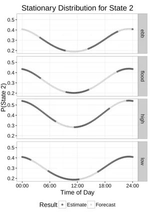
and highest from 21:00 – 1:00. In Figure 6, we see that the shark was more active during high tide in 401

general when compared to flood, low or ebb tide. While the equilibrium (or stationary) distribution 402

associated with low and ebb tide overlap, the state-dwell probabilities, i.e. the diagonal entries of the 403

t.p.m. corresponding to the probability of remaining in the same state, are higher during ebb tide than 404

in low tide. Naturally in a short time series the tide levels will be correlated with certain times of the 405

day, but a longer time series or a joint modelling of multiple time series, with tide levels observed during 406

all times of day, can provide robust estimates of the effect of tide on activity level using the HMM 407

formulation provided here. 408

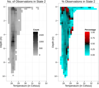
Using the Viterbi algorithm, we decoded the optimal state sequence to underlie the ODBA time 409

series. To further understand the effect of vertical habitat on behaviour, we related the decoded state 410

sequence to a grid of depth and temperature values, shown in Figure 7. The shark spent most of its time 411

over the nearly five day period in depths of about 3-6 metres and between 28-29◦C, with some higher 412

counts also in shallower waters, which is reflected in the state 2 counts. However, the percentages of 413

state 2 observations reveals that the shark was generally more active when near the surface in waters of 414

28-29◦C. There was generally less active behaviour exhibited when the individual was in very shallow 415

warm water (>29◦C). 416

5

Discussion

417

We detailed two approaches for analysing animal accelerometer data with HMMs: a supervised learning 418

approach for state prediction, such that classification is of primary interest, and an unsupervised learning 419

approach, where the states reflect biologically meaningful classes of behaviour, in order to infer drivers 420

of animal behaviour. The aim of a study and the type of data available will determine which of the two 421

is to be preferred. When the objective is to do classification and there is a set of pre-defined behaviours 422

of interest, then the model’s ability to correctly predict and categorize behaviours is of main interest. In 423

this instance, a supervised learning approach may be applied. One of the benefits of such an approach 424

Alternatively, if the objective is to infer (or, colloquially speaking, to ‘learn’) new aspects of animal 426

behaviour, then the unsupervised learning approach provides an excellent framework. The latter comes 427

with the implicit caveat that the states will not necessarily map directly to specific animal behaviours. 428

Any post-hoc behavioural interpretation of the estimated states is directly connected to the metric(s) 429

used, and must draw from background biological knowledge of the species of interest. In many cases, 430

behaviours such as foraging may not be exclusive to one state or another. Nonetheless, if the model is 431

able to identify bouts of behaviour which consistently re-appear, then it is often likely that these signify 432

something important in the animal’s behavioural repertoire and are worthy of further investigation. 433

Even when classification is the goal of an analysis, there are certainly practical scenarios which 434

preclude the use of an HMM, e.g. if the training data do not reflect the transitions between behaviours 435

or if there is insufficient data. Moreover, multiple studies have shown that other machine learning 436

algorithms, e.g. support vector machines (SVM) or random forests, can work well for classification of 437

animal acceleration data (Martiskainenet al., 2009; Nathanet al., 2012; Carrollet al., 2014; Grafet al., 438

2015). However, disregarding the serial dependence in the acceleration data usually is an unrealistic 439

assumption, which often goes unmentioned or is treated as an afterthought. Adopting the assumption 440

of independence is particularly risky if inferential statistics are applied to the output of say a machine 441

learning algorithm. In these cases, secondarily applied statistical tests will implicitly assume that 442

the machine learning categorizations contain more information content than is warranted, potentially 443

leading to spurious results. This is not just a statistical nuance and can be a crucial point. Such tests 444

are often applied as decision making tools to sort out “what matters” and setting the direction for 445

much further research effort. Also, in assuming independence, one allows for classifications that may 446

not be biologically realistic or must filter the classifications to properly identify a specific behaviour. 447

For instance, Carroll et al. (2014) used a SVM where one of the primary interests was to identify 448

prey handling/capture for penguins at sea. To confirm a prey capture event, they ruled that if the 449

SVM classified three consecutive observations as prey-handling this counted as a true prey capture. In 450

contrast, an HMM would have bypassed the need to filter through the classification results by accounting 451

for the serial dependence in observations corresponding to prey handling. In general, many behaviours 452

persist over longer stretches of time than those at which the data is processed, also necessitating the 453

use of a model that can account for the serial dependence. It may be difficult for any machine learning 454

algorithm that assumes independence to properly classify a sequence of observations into the same class, 455

unless the boundaries between classes are well-defined. In the context of recognition tasks, e.g. speech 456

or pattern recognition, HMMs have proven to be extremely successful tools for classification precisely 457

because they do account for the serial dependence in the signal of interest (Rabiner, 1989). 458

In the literature, inference on behavioural state-switching dynamics has sometimes been made using 459

two-stage (or even three-stage) analyses, where HMMs (or other machine learning algorithms) are used to 460

decode the behaviours underlying given observations, and subsequently a logistic regression is conducted 461

appeal of such an approach lies in the ease of implementation: fairly basic HMMs, without covariates, 463

are fitted to the accelerometer data and used to decode the states, and, subsequently, standard regression 464

software packages can be used to conduct a regression of the behavioural states on covariates. However, 465

it is our view that such a multi-stage analysis is less suited to relating accelerometer data to covariates 466

than the joint modelling approach presented in Section 3.3, for two reasons: (i) in the multi-stage 467

analyses, the uncertainty in state estimates is usually not propagated through the different stages of 468

analysis, and (ii) a regression analysis on decoded states needs to take into account the high serial 469

correlation in those states. Rather than ignoring these issues or trying to address them within a multi-470

stage analysis (which will render such an approach technically challenging), a direct joint modelling 471

approach, where neither of the problems arise, seems preferable. 472

Using a direct joint modelling approach in Section 4 we were able to learn about the effects that 473

atmospheric variables have on activity levels of a soaring raptor, while for the blacktip reef shark 474

we examined temporal and tidal inputs effects on its activity levels. The HMM produced similar 475

temporal patterns of activity to a previous analysis of the blacktip reef shark data set using GAMMs 476

(Papastamatiouet al., 2015). Both analytical methods revealed crepuscular and/or nocturnal increases 477

in activity with a tidal component, with the shark most active at the high tide or as tide was about to 478

ebb. By incorporating swimming depth and temperature, it was also revealed that highest activity was 479

seen when the shark was at the surface in waters of 28-29◦_{C. More importantly, the analysis showed that}

480

the shark was inactive when in very warm (>29◦C) shallow water or deeper water. These results agree 481

with a previous hypothesis that sharks are ‘hunting warm, and resting warmer’ and use warmer water 482

(> 29 ◦C) to increase the rate of some physiological function such as digestion, and not for foraging 483

(see Papastamatiouet al., 2015). The HMM in this case allows us to explain the drivers of activity in 484

the shark and move beyond just describing its movements, but rather explain ‘why’ it may be moving 485

or selecting certain habitats. The HMM also provided a measure of the change in probability of the 486

individual being in active states. Although there was a clear temporal pattern of activity, the HMM 487

identified the shark as 30% more likely to be in an active state during the late evening hours. For the 488

adult black eagle, the HMM provided a direct modelling approach to examine the effect of wind speed 489

and temperature on its activity level. The results suggests that the black eagle spent more time in the 490

relatively active state overall, and was more likely active in windier conditions. These results are in line 491

with theoretical (Pennycuick, 1972) and empirical (Lanzoneet al., 2012) studies. 492

We have covered the basic HMM framework here, but the popularity of the HMM framework is 493

due in part to its many extensions. In particular, there are two HMM extensions that have been 494

proven useful in classification of human activities: the hidden semi-Markov model (HSMM) (Langrock 495

& Zucchini, 2012) and the hierarchical hidden Markov model (HHMM) (Fineet al., 1998). The HSMM 496

models the time spent within a state by some probability distribution with support on the positive 497

real integers, thereby allowing for more complex state dwell time distributions than can be provided 498

spent in a resting behaviour adequately if the animal is known to rest for long periods of time. The 500

HHMM provides the framework necessary to identify composite behaviours. For instance, lunge feeding 501

in baleen whales is a composite behaviour made up of (1) initial increase in acceleration with (2) a 502

positive pitch angle, as animals commonly approach prey schools from below, followed by (3) a rapid 503

deceleration after the whale opens its mouth increasing its drag (Owenet al., 2015). The HHMM models 504

each composite behaviour as its own HMM, and models the transitions between composite behaviours, 505

i.e. switches between HMMs. 506

6

Acknowledgements

507

YYW was funded by Grants-in-Aid for Scientific Research from the Japan Society for the Promotion of 508

Science (grant reference 25850138). TP was supported by a South African National Research Foundation 509

Scarce Skills postdoctoral research fellowship, and TP and YPP received funding from the MASTS 510

pooling initiative (The Marine Alliance for Science and Technology for Scotland) and their support is 511

gratefully acknowledged. MASTS is funded by the Scottish Funding Council (grant reference HR09011) 512

and contributing institutions. TP and MM gratefully acknowledge the hardware, software, support 513

and expertise contributed by Prof. Willem Bouten and his research group UvA-BiTS (University of 514

Amsterdam Bird Tracking System). The authors are grateful to Orr Spiegel, the Associate Editor and 515

an anonymous referee for their useful comments that substantially improved the manuscript. 516

7

Data Accessibility

517

Data deposited in the Dryad repository: http://datadryad.org/resource/doi:10.5061/dryad.6bm2c 518

References

519

´

Akos, Z., Nagy, M., Leven, S. & Vicsek, T. (2010) Thermal soaring flight of birds and unmanned aerial 520

vehicles. Bioinspiration & Biomimetics,5, 045003. 521

Altun, K., Barshan, B. & Tun¸cel, O. (2010) Comparative study on classifying human activities with 522

miniature inertial and magnetic sensors.Pattern Recognition,43, 3605–3620. 523

Bao, L. & Intille, S.S. (2004) Activity recognition from user annotated acceleration data. Pervasive 524

computing, pp 1–17. Springer, Berlin Heidelberg. 525

Bouten, W., Baaij, E.W., Shamoun-Baranes, J., Camphuysen, K.C.J. (2013) A flexible GPS tracking 526

system for studying bird behaviour at multiple scales. Journal of Ornithology,154, 571-–580. 527

Broekhuis, F., Gr¨unew¨alder, S., McNutt, J.W. & Macdonald, D.W. (2014) Optimal hunting conditions 528

Brown, D., Kays, R., Wikelski, M., Wilson, R. & Klimley, A.P. (2013) Observing the unwatchable 530

through acceleration logging of animal behavior. Animal Biotelemetry,1, 1–16. 531

Campbell, H.A., Gao, L., Bidder, O.R., Hunter, J. & Franklin, C.E. (2014) Creating a behavioural 532

classification module for acceleration data: using a captive surrogate for difficult to observe species. 533

Journal of Experimental Biology,216, 4501–4506. 534

Carroll, G., Slip, D., Jonsen, I. & Harcout, R. (2014) Supervised accelerometry analysis can identify 535

prey capture by penguins at sea.Journal of Experimental Biology,217, 4295–4302. 536

Elliott, K.H., Le Vaillant, M., Kato, A., Speakman, J.R. & Ropert-Coudert, Y. (2013) Accelerometry 537

predicts daily energy expenditure in a bird with high activity levels.Biology letters,9, 20120919. 538

Fine, S., Singer, Y. & Tishby N. (1998) The hierarchical hidden Markov model: Analysis and applica-539

tions.Machine Learning,32, 41–62. 540

Gleiss, A.C., Wilson, R.P. & Shepard, E.L.C. (2011) Making overall dynamic body acceleration work: 541

on the theory of acceleration as a proxy for energy expenditure. Methods in Ecology and Evolution, 542

2, 23–33. 543

Gleiss, A.C., Wright, S., Liebsch, N., Wilson, R.P. & Norman, B. (2013) Contrasting diel patterns in 544

vertical movement and locomotor activity of whale sharks at Ningaloo Reef. Marine Biology, 160, 545

2981–2992. 546

Graf, P.M., Wilson, R.P., Qasem, L., Hackl¨ander, K. & Rosell, F. (2015) The use of acceleration to 547

code for animal behaviours; A case study in free-ranging Eurasian beavers Castor fiber.PLoS ONE, 548

10, e0136751. 549

Hart, T., Mann, R., Coulson, T., Pettorelli, N. & Trathan, P.N. (2010) Behavioural switching in a 550

central place forager: patterns of diving behaviour in the macaroni penguin (Eudyptes chrysolophus). 551

Marine Biology,157, 1543–1553. 552

Hastie, T., Tibshirani, R. & Friedman, J. (2001)The Elements of Statistical Learning, New York, NY: 553

Springer. 554

He, J., Li, H. & Tan, J. (2007) Real-time daily activity classification with wireless sensor networks 555

using hidden Markov model. Engineering in Medicine and Biology Society, 2007. EMBS 2007. 29th 556

Annual International Conference of the IEEE, pp. 3192–3795. IEEE. 557

Heerah, K., Hindell, M., Guinet, C. & Charrassin, J.B. (2014) A new method to quantify within dive 558

foraging behaviour in marine predators. PLoS ONE, 9, e99329. 559

Iwata, T., Sakamoto, K.Q., Edwards, E.W.J., Staniland, I.J., Trathan, P.N., Goto, Y., Sato, K., Naito, 560

Y. & Takahashi, A. (2015) The influence of preceding dive cycles on the foraging decisions of Antarctic 561

Katzner, T., Johnson, J.A., Evans, D.M., Garner, T.W.J., Gompper, M.E., Altwegg, R., Branch, T.A., 563

Gordon, I.J. & Pettorelli, N. (2013) Challenges and opportunities for animal conservation from re-564

newable energy development.Animal Conservation,16, 367–369. 565

Konishi, S. & Kitagawa, G. (2008) Information Criteria and Statistical Modeling, New York, NY: 566

Springer. 567

Langrock, R., King, R., Matthiopoulos, J., Thomas, L., Fortin, D. & Morales, J.M. (2012) Flexible and 568

practical modeling of animal telemetry data: hidden Markov models and extensions. Ecology, 93, 569

2336–2342. 570

Langrock, R., Kneib, T., Sohn, A. & DeRuiter, S.L. (2015) Nonparametric inference in hidden Markov 571

models using P-splines. Biometrics,71, 520–528. 572

Langrock, R. & Zucchini, W. (2012) Hidden Markov models with arbitrary state dwell-time distributions. 573

Computational Statistics and Data Analysis,55, 715–724. 574

Lanzone, M.J., Miller, T.A., Turk, P., Brandes, D., Halverson, C., Maisonneuve, C., Tremblay, J., 575

Cooper, J., O’Malley, K., Brooks, R.P. & Katzner, T. (2012), Flight responses by a migratory soaring 576

raptor to changing meteorological conditions Biology Letters,8, 710–713. 577

Leenders, N.Y.J.M., Sherman, W.M. & Nagaraja, H.N. (2000) Comparisons of four methods of estimat-578

ing physical activity in adult women.Medicine & Science in Sports & Exercise,32, 1320–1326. 579

Leos-Barajas, V., Photopoulou, T., Langrock, R., Patterson, T.A., Watanabe Y.Y., Murtroyd, M., 580

Papastamatiou, Y. (2016) Data from: Analysis of animal accelerometer data using hidden Markov 581

models. Methods in Ecology and Evolution doi:10.5061/dryad.6bm2c 582

MacDonald, I.L. (2014) Numerical maximisation of likelihood: A neglected alternative to EM? Inter-583

national Statistical Review,82, 296–308. 584

Mannini, A. & Sabatini A.M. (2010) Machine learning methods for classifying human physical activity 585

from on-body accelerometers.Sensors,10, 1154–1175. 586

Mannini, A. & Sabatini A.M. (2011) Accelerometry-based classification of human activities using Markov 587

modeling.Computational Intelligence and Neuroscience,2011, 647858. 588

Martiskainen, P., J¨arvinen, M., Sk¨on, J., Tiirikainen, J., Kolehmainen, M. & Mononen, J. (2009) Cow 589

behaviour pattern recognition using a three-dimensional accelerometer and support vector machines. 590

Applied Animal Behaviour Science,119, 32–38. 591

McKellar, A.E., Langrock, R., Walters, J.R. & Kesler, D.C. (2015) Using mixed hidden Markov models 592

Naito, Y. Bornemann, H., Takahashi, A, McIntyre, T. & Pl¨otz, J. (2010) Fine-scale feeding behavior of 594

Weddell seals revealed by a mandible accelerometer.Polar Science,4, 309–316. 595

Nathan, R., Spiegel, O., Fortmann-Roe, S., Harel, R., Wikelski, M. & Getz, W. (2012) Using tri-axial 596

acceleration data to identify behavioral modes of free-ranging animals: general concepts and tools 597

illustrated for griffon vultures. The Journal of Experimental Biology, 215, 986–996. 598

Owen, K., Dunlop, R.A., Monty, J.P., Chung, D, Noad, M.J., Donnelly, D., Golditzen, A.W. & Macken-599

zie, T. (2015) Detecting surface-feeding behavior by rorqual whales in accelerometer data. Marine 600

Mammal Science,32, 327–348. 601

Papastamatiou, Y.P., Watanabe, Y.Y., Bradley, D., Dee, L.E., Lowe, C.G. & Caselle, J. (2015) Drivers 602

of daily routines in an ectothermic marine predator: hunt warm, rest warmer? PLoS ONE, 10, 603

e0127807. 604

Patterson, T.A., Basson, M., Bravington, M.V. & Gunn, J.S. (2009) Classifying movement behaviour 605

in relation to environmental conditions using hidden Markov models.Journal of Animal Ecology,78, 606

1113–1123. 607

Pennycuick, C. J. (2008)Modelling the Flying Bird London: Academic Press, Elsevier. 608

Pennycuick, C. J. (1972) Soaring behaviour and performance of some east african birds, observed from 609

a motor-glider Ibis,114, 178-–218. 610

Phillips, J.S., Patterson, T.A., Leroy, B., Pilling, G.M. & Nicol, S.J. (2015), Objective classification 611

of latent behavioral states in bio-logging data using multivariate-normal hidden Markov models. 612

Ecological Applications, 25(5), 1244–1258. 613

Qasem, L., Cardew, A., Wilson, A., Griffiths, I., Halsey, L.G., Shepard, E.L.C., Gleiss, A.C. & Wilson, 614

R. (2012) Tri-axial dynamic acceleration as a proxy for animal energy expenditure; Should we be 615

summing values or calculating the vector? PLoS ONE,7, e31187. 616

Rabiner, L.R. (1989), A tutorial on hidden Markov models and selected applications in speech recogni-617

tion.IEEE Proceedings, 77, 257–286. 618

Ravi, N., Dandekar, N., Mysore, P. & Littman, M.L. (2005) Activity recognition from accelerometer 619

data. American Association for Artifical Intelligence,5, 1541–1546. 620

Sakamoto, K.Q., Sato K., Ishizuka, M., Watanuki, Y., Takahashi, A., Daunt, F. & Wanless, S. (2009) 621

Can ethograms be automatically generated using body acceleration data from free-ranging birds? 622

PLoS One,4, e5379. 623

Sato, K., Daunt, F., Watanuki, Y., Takahashi, A. & Wanless, S. (2008) A new method to quantify prey 624

acquisition in diving seabirds using wing stroke frequency.The Journal of Experimental Biology,211, 625

Sato, K., Mitani, Y., Cameron, M.F., Siniff, D.B. & Naito, Y. (2003) Factors affecting stroking patterns 627

and body angle in diving Weddell seals under natural conditions.The Journal of Experimental Biology, 628

206, 1461–1470. 629

Shepard, E.L.C., Wilson, R., Quintana, F., Laich, A.G., Liebsch, N., Albareda, D.A., Halsey, L.G., 630

Gleiss, A., Morgan, D., Myers, A.E., Newman, C. & Macdonald, D. (2008) Identification of animal 631

movement patterns using tri-axial accelerometry.Endangered Species Research,10, 47–60. 632

Simon, M., Johnson, M. & Madsen, P.T. (2012) Keeping momentum with a mouthful of water: behavior 633

and kinematics of humpback whale lunge feeding.The Journal of Experimental Biology, 215, 3786– 634

3798. 635

Suzuki, I., Naito, Y., Folkow, L.P., Nobuyuki, M. & Blix, A.B. (2009) Validation of a device for accurate 636

timing of feeding events in marine animals. Polar Biology,32, 667–671. 637

Watanabe, Y.Y., Lydersen, C., Fisk, A.T. & Kovacs, K.M. (2012), The slowest fish: swim speed and 638

tail-beat frequency of Greenland sharks. Journal of Experimental Marine Biology and Ecology,426, 639

5–11. 640

Watanuki, Y., Niizuma, Y., Gabrielsen, G.W., Sato, K. & Naito, Y. (2003), Stroke and glide of wing-641

propelled divers: deep diving seabirds adjust surge frequency to buoyancy change with depth. Pro-642

ceedings of the Royal Society of London B,270, 483–488. 643

Ward, J.A., Lukowicz, P., Troster, G. & Starner, T.E. (2006) Activity recognition of assembly tasks 644

using body-worn microphones and accelerometers.Pattern Analysis and Machine Intelligence, IEEE 645

Transactions,28, 1553–1567. 646

Williams, H.J., Shepard, E.L.C., Duriez, O. & Lambertucci, S.A. (2015) Can accelerometry be used to 647

distinguish between flight types in soaring birds? Animal Biotelemetry,3, 1–11. 648

Wilson, R.P., Shepard, E.L.C. & Liebsch, N. (2008) Prying into the intimate details of animal lives: use 649

of a daily diary on animals.Endangered Species Research,4, 123–137. 650

Wilson, R.P., White, C.R., Quintana, F., Halsey, L.G., Liebsch, N, Martin, G.R. & Butler, P.J. (2006) 651

Moving towards acceleration for estimates of activity-specific metabolic rate in free-living animals: 652

the case of the cormorant. Journal of Animal Ecology,75, 1081–1090. 653

Ydesen, K.S., Wisniewska, D.M., Hansen, J.D., Beedholm, K., Johnson, M. & Madsen, P.T. (2014) 654

What a jerk: prey engulfment revealed by high-rate, super-cranial accelerometry on a harbour seal 655

(Phoca vitulina).The Journal of Experimental Biology,217, 2239–2243. 656

Zucchini, W., MacDonald, I.L. & Langrock, R. (2016), Hidden Markov Models for Time Series: An 657

8

Supporting Information

659

Supporting Information Description

Appendix Further mathematical details for HMMs.

(Pseudo-)residual plots and model checking for both HMM applications presented in manuscript.

Comparing Supervised Learning Approaches

A comparison of four supervised learning ap-proaches when there is varying levels of auto-correlation present in the data.

9

Tables & Figures

Model Log-likelihood AIC ∆ AIC BIC ∆ BIC

No covariates 2000.2 -3980.4 21.6 -3929.4 21.6

Temperature 2001.9 -3979.9 22.1 -3918.6 17.0

Wind speed 2010.4 -3996.9 5.1 -3935.6 0

Wind speed, Temperature 2011.6 -3995.2 6.8 -3923.7 11.9

Wind speed, Temperature, 2017.0 -4002.0 0 -3920.3 15.3

Wind speed * Temperature

Model Log-likelihood AIC ∆ AIC BIC ∆ BIC

No covariates 639299.2 -1278370 779 -1277178 692

Time 639558.1 -1278872 277.2 -1277645 225

Time, High 639657.6 -1279063 86.2 -1277819 51

Time, High, Flood 639695.2 -1279130 19 -1277869 1

Time, High, Flood, Ebb 639708.7 -1279149 0 -1277870 0

0 1 2 3

17 Apr 18 Apr 19 Apr 20 Apr 21 Apr 22 Apr 23 Apr 24 Apr

Date

MSA

MSA values for 16 to 24 April

0 1 2 3

07:00 11:00 15:00 19:00

Time of day

MSA

MSA values for 21 April

0 20 40 60

0.0 0.5 1.0 1.5 2.0

Minimum specific acceleration (MSA)

Density

State−Dependent MSA Densities

4e−04 8e−04

2.00 2.25 2.50 2.75 3.00

Minimum specific acceleration (MSA)

Density

Tail behaviour of Densities

0 10 20 30 40

0.0 0.5 1.0 1.5 2.0

Minimum specific acceleration (MSA)

Density

Densities

Marginal State 1 State 2

Marginal MSA Density

0.00 0.25 0.50 0.75 1.00

0 2 4 6

Wind speed (m/sec)

Probability

State 1 −> State 1 State 2 −> State 2

State Dwell Probabilities

0.00 0.25 0.50 0.75 1.00

0 2 4 6

Wind speed (m/sec)

Probability

State 1 State 2

Stationary Distribution

0 2 4 6 8

13 Jul 00:00 13 Jul 06:00 13 Jul 12:00 13 Jul 18:00 13 Jul 24:00

Time of Day

ODBA

ODBA Values for 13 July, 2013

0e+00 5e−04 1e−03

2 4 6 8 10

Overall Dynamic Body Acceleration

Density

Tail Behaviour of Densities 0

5 10 15

0.0 0.5 1.0 1.5 2.0

Overall Dynamic Body Acceleration

Density

State−Dependent ODBA Densities

0 5 10

0.0 0.5 1.0 1.5 2.0

Overall Dynamic Body Acceleration (ODBA)

Density

Density State 1 State 2 Marginal

Marginal ODBA Density

0.2 0.3 0.4 0.5

0.2 0.3 0.4 0.5

0.2 0.3 0.4 0.5

0.2 0.3 0.4 0.5

eb

b

flood

high

lo

w

00:00 06:00 12:00 18:00 24:00

Time of Day

P(State 2)

Result

Stationary Distribution for State 2

0

2

4

6

8

10

28 29 30 31 32 33

Temperature (in Celsius)

Depth (m)

0 500 1000 1500

Count

No. of Observations in State 2

0

2

4

6

8

10

28 29 30 31 32 33

Temperature (in Celsius)

Depth (m)

0.00 0.25 0.50 0.75 1.00

Percentage

% Observations in State 2