A Method to Search Traveling Salesman Problem
Backbones Based on GA and Frequency Graph
Yong Wang
*, Changxin Geng,
Yiwen Wu
School of Renewable Energy, North China Electric Power University, Beijing 102206, China.
* Corresponding author. Tel.: +8613611023249; email: [email protected] Manuscript submitted March 7, 2019; accepted May 20, 2019.
doi: 10.17706/jcp.14.6 426-437.
Abstract: The traveling salesman problem (TSP) is a well-known NP-hard problem in combinatorial optimization. The search space of the optimal Hamiltonian cycle (OHC) is increasing exponentially according to the scale n. In order to reduce the search space of TSP, we first convert the complete graph Kn
into the frequency graph (FG) with the approximate optimal n-vertex paths computed with an improved GA. The GA is improved with a four-vertex-three-line inequality to compute the approximate paths of TSP. Then, TSP backbones with 2n edges are derived from the FG. The experimental results show that the TSP backbones include at least 95% edges in the OHC. Based on the backbones, the search space of the OHC or approximations is greatly reduced.
Key words: TSP, Backbone, frequency graph, GA.
1.
Introduction
As is well-known, traveling salesman problem (TSP) is a famous NP-hard problem [1], which has attracted a lot of attention from researchers in various fields such as mathematics, computer science, bioinformatics, operations research, supply chain, etc. Since TSP represents a class of problems in the field of combinatorial optimization, the exploration of its accurate or approximate solution has always been an important direction in the design of algorithm [2]. There are two main kinds of algorithms for solving TSP in applications. One is the exact algorithms including the dynamic programming, branch and bound algorithm, cutting plane, etc. [3]. The other is the intelligent optimization algorithms, such as the GA, ACO, SA, PSO, etc. [4].
Finding the optimal solution for a small-scale TSP is simple. However, it is very difficult, most of the times impossible, for the big scale of TSP whose search space of the optimal Hamiltonian cycle (OHC) is very large. Because of the constraint conditions, we can solve the big scale TSP problem by integer programming and dynamic programming, but strong computer equipment is needed and the computation time is too long. It has been reported that Concorde package resolved the big scale TSP with 85900 cities [5]. The task was completed using 128 networked computer systems and consumed 1.2 years. The computation time is equal to 136 years of computing tasks using a computer.
graphs [6]. In a sparse graph, the search space of the original TSP can be significantly less than that in complete graphs. We call the sparse graphs containing the edges of OHC the TSP backbones.
In this research direction, Boese introduced the conception of backbones into the field of TSP in 1995 [7]. In 1998, Monasson discussed the backbones algorithm for the satisfiability problem (SAT) [8]. In 2003, Schneider found that the intersections of the local optimal solutions are similar to the TSP backbones [9]. Thus, the intersections of the local optimal solutions are regarded as the approximate backbones. Five kinds of local optimal algorithms including the random 2-opt, fast opt, fast 3-opt, LK and LSMC are tried by Professor Boese for the 532 vertices scale of TSP [10]. It is found that the intersections of the local optimal solutions computed by these algorithms occupy more than 80% edges in the globally optimal solution.
The previous backbones algorithms are used to solve TSP in recent years. The general backbones algorithms consist of two stages. In the first stage, the backbones are found from the complete graph. The ideal TSP backbones should contain as the least number of edges as possible but contain as many edges as possible in the OHC. In the second stage, the backbones algorithm is to find the optimal solution or approximations by finding the edge in the OHC and the approximations. The backbones algorithms are based on the big hole theory owing to Blum [11]. The theory has been proven by many experiments that there are many common edges between the global optimal solution and the local optimal solutions computed by the algorithms.
Based on big hole theory, several approximate solutions are computed with various algorithms. Then the edges among these approximations are enumerated. The frequency of an edge is the number of approximations containing this edge. Some of the intersected edges are preserved according to the frequency of the edges. After the enumeration of every edge from the approximations of TSP, the frequent graph (FG) is formed. In the FG, we can see the frequency of each edge in the different approximate solutions. A certain number of larger frequency edges are selected from FG, we can get the TSP backbones including the OHC or approximations. This is the basic idea of backbones principle based on FG. Since the backbones include small quantities of edges, the search space in the backbones is greatly reduced. The key problem is to compute a better backbone containing the OHC edges as many as possible.
There are many methods to compute TSP backbones. The previous methods generally compute the shortest distance of several vertices firstly, then the frequency of edges in these approximate solutions is computed. At last, the heuristic rules are used to compute the TSP backbones. these kinds of methods are characterized by fast speed but poor accuracy. If more vertices are selected to calculate the shortest distance, the complexity will be increased and the accuracy will be further improved. As the number of vertices increases, it is difficult to solve the shortest distance between them, so heuristic intelligent algorithm is needed.
Among the algorithms to compute the approximations, genetic algorithm (GA) is one of the most effective meta-heuristic methods, which is widely used in optimization problems [12]. GA simulates the natural selection of Darwinian evolution and the biological evolution of the genetic mechanism. GA was first proposed by professor JH Holland in 1975 [13]. The implicit parallelism of the algorithm promotes the global optimization performance [14]. According to the probability rules, the search direction can be adjusted automatically to the optimal solution. Compared with the traditional methods for TSP, GA has the good ability of convergence based on the evolutionary rules. Compared with the other heuristics, when the accuracy of solutions is required, it needs the smaller computing time and has the higher robustness.
group. This problem is usually confronted when we use the GA to resolve the complex problems.
Because the large amount of time is consumed to calculate the better approximations, the above methods use a limitative number of approximations to compute the TSP backbones. Unlike previous methods, a large number of approximate optimal n-vertex paths are computed with the improved GA. The GA is improved by incorporating the four-vertex-three-line inequality to compute the better approximate optimal n-vertex paths. Then, the frequency of edges is enumerated from these approximate optimal n-vertex paths. At last, the TSP backbones are computed based on the edge frequency.
The rest of the paper is organized as follows. The frequency graph is introduced in section 2. The conception of optimal k-vertex paths (OPk) is given and the number of which is formulated. Section 3
describes the improved GA for computing the approximate optimal n-vertex paths of TSP. In section 4, we computed the frequency graph by approximate optimal n-vertex paths and the backbones are computed based on the frequency graph. In section 5, we shall do experiments to compute the backbones for some TSP instances in the TSPLIB. In the end, the conclusions are drawn as well as the future research directions are given.
2.
The Frequency Graph for TSP
A TSP graph is generally represented as G= (V, E). The vertex set is V= (v1, v2, v3, ... vi, ..., vn) and the edge
set is E= (e1×2, e1×3, ..., e(n-1) ×n). vi (1≤i≤n) represents the vertex and eij (1≤i, j≤n) is the edge that links the two
vertices vi and vj. A sparse graph G can be represented by an adjacent matrix A(G)={ai×j} (1≤i, j≤ n). If an
edge eij is in the sparse graph, the element aij=1. Otherwise, aij=0. We devote to computing the sparse graph
including as many as edges in OHC.
We firstly explain the relationships between the HCs and the k-vertex paths. For n-vertex TSP, an HC is represented as HC = (v1, v2, v3, ... vi, ..., vn, v1) whose two terminal vertices are identical. It is obviously that
the HC is made up of some k-vertex paths (P). A k-vertex path can be represented as Pk = (v1, v2, ... vk-1, vk)
(2≤ k< n). There are two terminal vertices at both ends and the other vertices are in the middle. The number of vertices in the Pk is noted with the superscript k. The Pks in the OHC are different from most of
the other Pks. In general, they are much shorter than most of the other Pks. We call the Pks in the OHC as the
optimal k-vertex paths (OP). Any one OPk is represented as OPk= (v1, v2, ..., vk-1, vk). For any one OPk in the
OHC, its two terminal vertices are determined. Furthermore, the OPk is shorter than the other Pks
containing the same set of vertices and the two identical terminal vertices. Given a set of k vertices in a weight graph, there are k×(k-1)/2 OPks if their two terminal vertices are determined. The weight of OPk is
minimal compared with the other Pks with the same vertices and two terminal vertices.
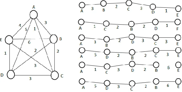
In Fig. 1, an OPk is illustrate by a simple weighted graph (WG) with 5 vertices A–E where k=5. The weight
of the edge is the number on the side. There are 5! / 2 P5s composed of the five vertices and there are 10
OP5s for symmetric TSP. If we take the vertices A and E as the two terminal vertices, there are six P5s and
the shortest P5 is the OP5 for vertices A and E. In Fig. 1, the weights of the six paths (A, B, C, D, E), (A, B, D, C,
E), (A, C, B, D, E), (A, D, B, C, E), (A, C, D, B, E), (A, D, C, B, E) are 9 ,11, 6, 12, 12 and 16, respectively. Obviously, the path (A, C, B, D, E) is the OP5 whereas the rest of the five paths are general P5s. Since the OP5
= (A, C, B, D, E) is shortest, it has the potential to be included in the OHC. The number of Pks is computed as equation (1) for symmetrical TSP.
= ! 2 k k n P k
N C (1)
The number of OPks is computed as formula (2).
−
= ( 1)
2 k k n OP k k
N C (2)
where k n
C in equation (2) is the combination number in the case that k vertices are selected from n vertices. The number of OPk is much smaller than the number of Pks. The number of OPks rises first if k ≤ n/2+1 for
even number n and k ≤ (n ± 1)/2+1 for odd number n. Then, it decreases according to k. There is a maximal number when k=n/2+1 for even number n (k= (n ± 1)/2+1 for odd number n). For symmetrical TSP, the total number of OPk is computed as formula (3).
−
= =
=
=
− = − 32 2
1
( 1) ( 1)2
2 k n n k n n OP k k
N N k k C n n (3)
As the number of vertices is creasing, the total number of OPk increases exponentially according to n. The
Pks excluding from the OPks are the non-OPks (NOP). They will become shorter if we exchange their
intermediate vertices. It is clear that the number of NOPs is much bigger than that of the OPks once k is
bigger than 4. As we know, the NOPs do not belong to OHC.
Given a number of OPks, the OPks have the potential to form OHC as well as the edges in OPks. However,
there is no doubt that not all edges are belonging to the OHC. Therefore, we need to find a way to distinguish the edges in OHC from the other edges. There is an applicable method to screen out them based on the frequency of the edges.
The OHC is made up of some edges. We pay more attention to the frequency of edges computed with OPks.
An FG is computed by a set of Pks or OPks. The frequencies of edges are much distinctive due to the selection
of OPks. The FG is computed as follows [6]. Given a set of Pks (or OPks) and k>2, the frequency of each edge is
computed from them. The frequency of edge is the number of the Pks (or OPks) containing this edge.
The edges of OHC are concerned. Given a set of OPks with more than 2 vertices, the frequencies of the
edges are enumerated and an FG is computed. In an FG, the numbers on the edges are their frequencies enumerated from the set of OPks. If the FG is computed with the OPks, the edges with the big frequency are
regarded. Based on the frequency of edges, most of the useless edges will be ignored as one chooses the OHC edges from the FG. In this paper, these selected edges are taken as part of the TSP backbones, in which there's a big proportion of OHC edges.
included in all of the OPks belong to OHC and the frequencies of them are maximal. The sparse graph
includes all the OHC edges which is also the TSP backbones. The approximate solution or accurate solution can be found in the spare graph. However, not all edges of big frequency belong to OHC due to selection of the various OPks. Therefore, we aim to compute the sparse graphs that contain the most number of OHC
edges and are tried to preserve the least number of useless edges.
3.
FG computed with the Improved GA
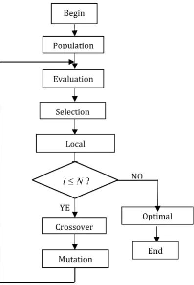
In this section, the general GA is improved with the four-point three-line inequality to compute the OPns or approximate OPns to compute the FG. Since computing the OPns is as hard as computing the OHC, the GA is improved with a four-vertex-three-line inequality to compute the OPns or approximate OPns. The approximate OPns also have many intersections of edges with the OHC if the approximate OPns approach the OHC. The frequency of the OHC edges will be much bigger than most of the other edges if they are computed with the approximate OPns. The procedure of the improved GA to compute the OPns or approximate OPns is shown in Fig. 2. Besides the five operations of the chromosome coding, crossover, variation, evaluation and selection in the traditional GA, the four-point three-line local optimization strategy is also included.
Fig. 2. The improved GA to compute FG.
The implementation of each operation in the improved GA is described as follows.
Step 1: Chromosome Encoding. The vertices are noted as integers. Each digit represents a vertex. A group of sequences containing the vertices are generated randomly and they are taken as the population of GA. Each sequence represents a Hamiltonian path of TSP. The number of iterations (N) and the number of the population are given at this stage.
Step 2: Fitness Evaluation. The objective function of TSP is the distance of the travelling tour. The reciprocal of a path length L is considered as the fitness function, i.e., 1/L. The greater the fitness value of the individual path is, the shorter the individual path is and the better the path is. In GA, a better path (also
Mutation
NO
Optimal solution
End YE
S Local optimization
Selection Evaluation
Crossover
as the chromosome) is more likely to be selected to the next generation.
Step 3: Selection. Selection is the process of generating new population from a previous generation of individuals with strong vitality. According to fitness function, individuals (paths) with bigger fitness values are more likely to go into the next generation. The process is the imitation of natural selection. In this paper, the method of truncation selection is adopted to ensure the global convergence of the GA and the individual diversity of the population. Here the elitist strategy will be considered. In this process, the best path in the population is always guaranteed to pass to the next generation.
Step 4: Crossover. The so-called crossover operation means that two pairs of paths exchange some parts of their genes (path fragments) in order to form two new individuals. The paths exchange their segments with each other according to the cross probability. Two individuals in population are chosen at random firstly. Secondly, the exchanged partial paths in the two individuals are selected with the random method. Thirdly, the two individuals exchange the selected partial paths according to crossover probability to generating two new individuals.
Step 5: Mutation. The basic content of the mutation operation is to change some of the genes of the individual in the population. First, the mutation probability is determined according to the mutation probability. The vertices in different path positions are chosen at random. Then the vertices change their positions to form a new path.
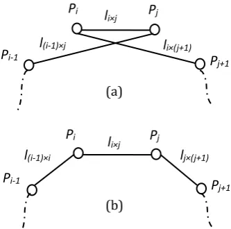
Step 6: Local optimization. In the GA, after cross, mutation, and the evaluation of paths, there are still non-optimal local paths in the whole path. If we use the local optimization methods, these long local paths can become shorter so as to compute the better paths. To enhance the traditional GA, the four-point-three-line inequality is as the local optimization to compute better paths after the evaluation stage. The principle of the local search algorithm is illustrated in Fig. 3.
There are two paths (a) and (b) in Fig. 3. The path (a) contains the local path (Pi-1, Pj, Pi, Pj+1) whereas the
path (b) includes the local path (Pi-1, Pi, Pj, Pj+1). Each local path is composed of four vertices and three lines
where li× j is the length of edge ei× j between the vertices Pi and Pj (2≤i≤n, 1≤j≤n-1). Except for the two local
paths, we assume the paths (a) and (b) contain the other identical local path and the length is noted as Lrest.
Provided that the path (b) is the optimal solution it’s obvious that the inequality l(i-1) ×j+ li× j+ li×(j+1)≥ l(i-1) × i+
li× j+ lj×(j+1) holds. This is the four-point-three-line inequality. According to the inequality, we can exchange
the positions of vertices Pi and Pj in path (a) to compute the better path (b).
(a)
(b)
Fig. 3. The principle of four-vertex- three-line inequality.
According to this principle, we can convert all the local paths containing 4 consecutive vertices into the shorter local paths so that the better paths will be computed. The four-point-three-line inequality is easy to
Pi-1
Pi Pj
Pj+1
l(i-1)×j
li×j
li×(j+1)
Pi-1
Pi Pj
Pj+1
li×j
implement and the computation time is O(n), which will improve the ability of GA to find the better results. From the experimental results, it is found that the improved GA improves the convergent speed and reduces the computational time. Moreover, the generated paths are more accurate for computing the frequency graph. The algorithm of the improved GA is given in Table 1 and Table 2.
The procedure of the improved GA with local search algorithm is presented in Algorithm 1.
Table 1. The Improved GA
Algorithm 1: improved GA for finding optimal or near-optimal OPns
01: Input the initialization parameters, population number P, iteration number N. 02: Generate the initialize population, initialize i =1
03: for i ≤ N do
04: Compute fitness of each chromosome and evaluation the population. 05: Perform the selection operation to choose a set of good individuals. 06: Perform crossover operation to generate hybrid individuals. 07: Perform mutation operation to generate mutated individuals.
08: Perform four-vertex-three-line inequality to compute better individuals. 09: End for
10: Output the solutions.
In summary, the FG is computed with the OPns or approximate OPns computed with the improved GA.
The procedure is given in Table 2.
Firstly, two end vertices are chosen as the end vertices of a Pns. The approximate optimal OPns between
the two vertices is computed by the improved GA. For n-vertex scale of TSP, not all pairs of vertices are used. Instead, we choose the n pairs of them to compute n OPns or approximate OPns, which greatly reduces
the amount of calculation time.
Secondly, the frequency of each edge is enumerated from the n the OPns or approximate OPns. After the
FG is obtained, the 2n edges with the biggest frequency are drawn from FG to construct a sparse graph as the backbones of the TSP.
Table 2. The Algorithm to Compute FG
Algorithm 2: computing FG based on Pks
01: While (termination criteria not satisfied) do 02: Generate two terminal vertices
03: Search the approximate OPns based on improved GA
04: End while
05: Compute the frequency of every edge 06: Select the candidate edges to form an FG 07: Output the FG
4.
TSP Backbones from FG
Backbone is a conception from statistical physics. Simply, backbone is the same part or structure as the optimal solution. Backbone is a very effective concept for NP-hard problems in combinatorial optimization. It is of great significance to measure the difficulty of hard problem. Slaney studied the relationship between backbones and the difficulty or cost of search for resolving hard problems. He found that the backbones were usually used to develop heuristic algorithms for resolving the combinatorial optimization problems [15].
sparse graph. The size significantly affects the difficulty of TSP. The larger the size is, the more difficult the algorithm is to compute the global optimal solution of TSP.
Since the backbones include a small number of edges, the search space of TSP is greatly reduced. Getting a better backbone for TSP becomes the research hot spot in recent years [16]. A good backbone generally contains the OHC edges as most as possible and the other edges as least as possible. Since it is usually difficult to obtain the OHC, many researchers try to compute backbones by indirect methods such as limit crossing [17]. However, the drawback is that it takes a long time and the method is not applicable in practice for big scale of TSP.
Given a TSP instance, we aim to save the OHC edges with a small computation cost. Here the FG is taken as the basis to figure out backbones of TSP. In an FG, the edges are sorted according to their frequencies from big to small values. Then the edges with big frequency are preserved as the OHC candidate edges to form a TSP backbone. After an FG is computed, this method is efficient. For example, the sorting algorithm requires O(n2logn) time. If kn edges with big frequency are maintained, the time complexity is O(n). Thus,
the computation of TSP backbone needs O(n2logn) computation time. Since the FG is computed with the approximate OPns, the OHC will have big frequency and most of them will be preserved in the backbone.
In Fig. 4. (a), a 10-vertex TSP is used to illustrate the performance of FG computed with approximate OPns
and conclude the backbone. The ten points are selected from the 31 main cities in China. The black lines represent the edges in complete graph and the green dash lines are the edges in OHC. Firstly, 10 pairs of terminal vertices are selected at random. Secondly, the approximate OPns is computed based on the
improved GA. In the improved GA, the number of population is 30, the number of iterations is 200, the fitness value is 2, and the probability of crossover and mutation is both 0.4. The frequencies of the edges are enumerated from the 10 approximate OPns. The FG is computed with these approximate OPns. Ten
edges with the highest frequency are selected from the FG to form the backbone as Fig. 4. (b). The number on an edge is the frequency in FG. The frequencies of the other edges are smaller than those of the ten edges in Fig. 4. (b). For evaluating the performance of the FG, we compute the OHC with the exact branch and bound method. It found that the backbone was just the OHC of the 10-vertex instance. The simple example displays the approximate OPns really have many intersected edges with the OHC. Therefore, it is feasible to
compute a backbone of TSP from the FG computed with the approximate OPns.
Fig. 4. (a) A 10-vertex TSP instance, (b) The backbone of the 10-vertex TSP.
For small scale TSP, the OPns is apt to compute. The OHC can be obtained by selecting the ten edges of the
highest frequency. With the vertex number increasing, the number of OPns will increase rapidly. Brutal
method is unable to compute the OPns. To compute a good TSP backbone, the approximate OPns are
computed with the improved GA and they are used to compute the FG. As the approximate OPns have many
that the backbone quality depends on the approximate OPns computed with the improved GA. The nearer
the approximate OPns approach the OHC, the better the performance of the FG is and the smaller the search
space of TSP is on the backbone.
5.
Example and Result
Some Euclidean TSP instances are used to validate the method. These TSP instances are downloaded from TSPLIB. The backbones containing a small number of edges are computed and the search space of OHC is significantly reduced. For comparison, the OHC of these instances are computed with Concorde package online owing to Mittelmann (NEOS Server for Concorde). The OHC edges are used to display how many OHC edges are contained in the backbones. The computation program is coded with MATLAB and the program is run on a DELL computer with 2.33GHz processor and 4G memory.
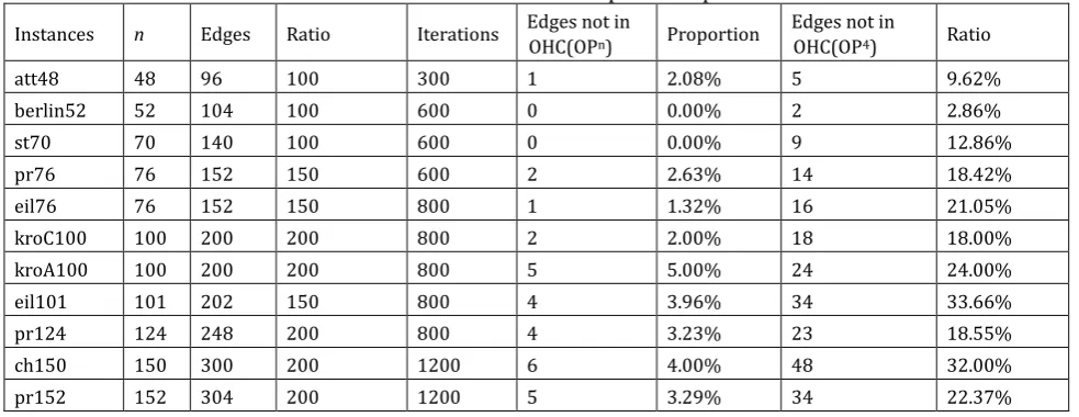
For each TSP instance, two vertices are randomly selected firstly as the terminal vertices. Then an approximate OPn is computed with the improved GA. In this way, total n OPns are computed for computing
an FG. Then, based on the FG, 2n edges with the biggest frequencies are selected to compose the TSP backbones. The experimental results are shown in Table 3. For these TSP instances, the backbones contain nearly all of the OHC edges and only a few OHC edges are lost. The backbones contain more than 95% of the OHC edges for these TSP instances. It means the improved GA computes the good approximate OPns. The
OHC edges have the bigger frequencies than most of the other as they are computed with these approximate OPns. As we maintain more edges with the big frequency, less OHC edges will be lost in the
backbones.
To show the advantage of using approximate OPns to compute the backbones, the OP4s are used to
compute the backbones for comparisons. For each TSP instance, 600,000 OP4s are chosen at random to
compute the frequency of edges at first. Then the 2n edges with the biggest frequencies are chosen to compose a sparse graph. The results illustrated that the sparse graphs lose a big portion of the OHC edges, see Table 3. It says the approximate OPns are better as a means to compute the backbones than the OP4s for
TSP.
Table 3. The Results of the Sparse Graphs
Instances n Edges Ratio Iterations Edges not in
OHC(OPn) Proportion
Edges not in
OHC(OP4) Ratio
att48 48 96 100 300 1 2.08% 5 9.62%
berlin52 52 104 100 600 0 0.00% 2 2.86%
st70 70 140 100 600 0 0.00% 9 12.86%
pr76 76 152 150 600 2 2.63% 14 18.42%
eil76 76 152 150 800 1 1.32% 16 21.05%
kroC100 100 200 200 800 2 2.00% 18 18.00%
kroA100 100 200 200 800 5 5.00% 24 24.00%
eil101 101 202 150 800 4 3.96% 34 33.66%
pr124 124 248 200 800 4 3.23% 23 18.55%
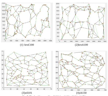
ch150 150 300 200 1200 6 4.00% 48 32.00%
(1) kroC100 (2)kroA100
(3)eil101 (4)ch150
Fig. 5. The backbones of kroC100, kroA100, eil101, ch150.
In Fig. 5, the backbones and the OHC of several typical examples are shown. The dotted green lines are the OHC of TSP and the solid black lines are edges in the backbones. One can find that the backbones include the majority edges in OHC. According to the experimental results, the TSP backbones can be selected by this method effectively, and the search space of OHC can be reduced. In the above method, we select 2n edges in the backbones. If more edges are selected in TSP backbones, the portion of the edges in OHC will be bigger.
6.
Conclusions and Future Work
TSP backbones are useful to reduce the computation time of TSP algorithms. The FG is taken as the basis to derive the TSP backbones according to the frequency of edges. The frequency of the OHC edges is generally much bigger than that of most of the other edges in an FG owing to the approximate OPns. The GA
is improved with a four-vertex-three-line inequality to compute the approximate OPns. The experimental
results for several TSP instances show that the backbones contain more than 95% edges in the OHC and they just contain 2n edges. We also compute the TSP backbones with a lot of OP4s. The backbones
computed with the approximate OPns are much better than the results computed based on OP4s. According
Acknowledgment
The authors acknowledge the funds supported by the Fundamental Research Funds for the Central Universities (No.2018ZD09 and 2018MS039).
References
[1] Mohiddinshaw, S., & Gurram, D. (2015). A note on computational approach to travelling sales man problem. International Journal of Computer Applications, 115(8), 975-8887.
[2] Kuo, I. H., Horng, S. J., Kao, T. W., Lin, T. L., Lee, C. L., Chen, Y. H., Pan, Y. I., & Terano, T. (2010). A hybrid swarm intelligence algorithm for the travelling salesman problem. Expert Systems, 27(3), 166–179. [3] Lin, S., & Kernighan, B. W. (1973). An effective heuristic algorithm for the TSP. Operations Research,
21(2), 498-516.
[4] Pan, G., Li, K., Ouyang, A., & Li, K. (2016). Hybrid immune algorithm based on greedy algorithm and delete-cross operator for solving TSP. Soft Computing, 20(2), 555-566.
[5] Lenstra, J. K., & Shmoys, D. B. (2009). Book review: The traveling salesman problem, a computational study (by D. L. Applegate, R. E. Bixby, V. Chvátal, W. J. Cook). Siam Review, 799-801.
[6] Wang, Y. (2015). An approximate method to compute a sparse graph for traveling salesman problem. Expert Systems with Applications, 42(12), 5150-5162.
[7] Boese, K. D., Kahng, A. B., & Muddu, S. (1994). A new adaptive multi-start technique for combinatorial global optimizations. Operations Research Letters, 16(2), 101-113.
[8] Monasson, R., Zecchina, R., Kirkpatrick, S., Selman, B., & Troyansky, L. (1999). Determining computational complexity from characteristic 'phase transitions.' Nature, 400(6740), 133-137.
[9] Schneider, J. (2003). Searching for backbones—A high-performance parallel algorithm for solving combinatorial optimization problems. Future Generation Computer Systems, 19(1), 121-131.
[10]Boese, K. D., Kahng, A. B., & Tsay, R. S. (1994). Scan chain optimization: Heuristic and optimal solutions. Internal Report Ucla Cs Dept.
[11]Blum, H. (1967). A transformation for extracting new descriptors of shape. Models for the Preception of Speech & Visual Form, 19, 362-380.
[12]Holland, J. H. (1987). Genetic algorithms and classifier systems: Foundations and future directions. Proceedings of International Conference on Genetic Algorithms on Genetic Algorithms and Their Application.
[13]Holland, J. H. (1973). Erratum: Genetic algorithms and the optimal allocation of trials. Siam Journal on Computing, 2(2), 88-105.
[14]Anderson-Cook, C. M. (1998). Practical genetic algorithms. Publications of the American Statistical Association, 100(471), 1099-1099.
[15]Slaney, J., & Walsh, T. (2001). Backbones in optimization and approximation. IN IJCAI-01, 254-259. [16]Zhang, W., & Looks, M. (2005). A novel local search algorithm for the traveling salesman problem that
exploits backbones. Proceedings of the Nineteenth International Joint Conference on Artificial Intelligence. Edinburgh, Scotland, UK
[17]Zhang, W. X. (2004). Phase transitions and backbones of the asymmetric traveling salesman problem. Journal of Artificial Intelligence Research, 21, 471-497.
aircraft at Nanjing University of Aeronautics and Astronautics, Nanjing, China. His research interests include combinatorial optimization, graph algorithms and applications in industrial engineering.
Changxin Geng was born in China in 1993. She received the B.S degree from North China Electric Power University (NCEPU), Beijing, China, in 2016. His main areas of research interest are combinatorial optimization, machines learningand intelligent algorithms. Mr. Geng is a member of theState Key Laboratory Of Alternate Electrical Power System With Renewable Energy Sources in NCEPU.