1
Reconstructing B-patch surface from triangular mesh
L.T.T.Nga
1,*, N.T.Khoi
2and N.T.Thuy
21,2Danang University of Science and Technology, Danang, Vietnam 3 VNU University of Engineering and Technology, Hanoi, Vietnam
Abstract
B-patch is the main block for creating the multivariate B-spline surfaces over triangular parametric domains. It has many interesting properties in the smooth surface construction with arbitrary topology. This paper proposes a new approach for reconstructing B-patch surfaces from triangular mesh based on a local geometric approximation, along with inverse subdivision scheme. The result B-patches with the low degree cross through most of the data points of the original meshes after some steps of the local geometric approximation. The accuracy of result surfaces can be carried out by changing the position of control points and adjusting knotclouds in each of the iterations. Some concrete experimental examples are also provided to demonstrate the effectiveness of the proposed method. Because most of the low degree parametric curves and surfaces are often employed in CAGD, this result has practical significance, especially for mesh compression, inverse engineering, and virtual reality.
Keywords: B-patch, geometric approximation, inverse subdivision, reconstruction, triangular mesh.
Received on 5 December 2017, accepted on 8 December 2017, published on 10 January 2018
Copyright © 2018 L.T.T.Nga et al., licensed to EAI. This is an open access article distributed under the terms of the Creative Commons Attribution licence (http://creativecommons.org/licenses/by/3.0/), which permits unlimited use, distribution and reproduction in any medium so long as the original work is properly cited.
doi: 10.4108/eai.10-1-2018.153547
*Corresponding author. Email: [email protected]
1. Introduction
Reconstructing the smooth surface from a set of data points is one of the significant research areas and has widely been applied in many fields of computer aided geometric design, reverse engineering, geometric modeling, vision, computer graphic, virtual reality, medical image segmentation [8][9]. Despite many difficulties and challenges such as mesh parameterization, construction of control polygon mesh, surface evaluation, etc; the smooth surface reconstruction remains an active research problem.
The surfaces over rectangular parametric domains, as tensor-product surfaces, include Bézier, B-spline, or NURBS…, inherit most of the desirable properties of univariate B-splines such as convex hull, intuitive and local control, and they have long become an excellent tool for modeling surfaces [8]. However, the complicated surfaces cannot sometimes be partitioned into quadrilaterals
naturally. Hence, the smooth surfaces of these objects are also difficult to be modeled by tensor product patches.
Comparing with the rectangular parametric surfaces, the surfaces over triangular domains flexibly allow joining and suit for modeling of surfaces with non-rectangular topological type because of the more natural way to partition a domain into triangular regions [4][12]. The bivariate splines on the triangular domain not only possess all the important properties of univariate B-splines but also have the lower polynomial degree [9]. On the other hand, because their control polyhedrons are triangular meshes, they provide multiscale resolution and conformity to complex geometries, allow for more flexible splicing and highly efficient processing [12][15]. B-patch surface is also a bivariate spline, which is defined over a triangular parametric domain. It is the main block for creating the multivariate B-spline surfaces. Consequently, this surface has many important properties for performing the surface of 3D objects flexibly.
This paper proposes a new approach for reconstructing the low degree B-patch surfaces from triangular meshes
Research Article
on Industrial Networks and Intelligent Systems
EAI Endorsed Transactions on Industrial Networks and Intelligent Systems
2 based on the local geometric approximation, along with the inverse subdivision scheme. The proposed method consists of three major steps. Firstly, a control polyhedron of the B-patch surface is generated by applying the inverse subdivision scheme. Next, the error vectors are evaluated for each data point of the given mesh. Finally, this surface is approximated to the original mesh based on these vectors. For improving the accuracy of reconstructed B-patch, control points and knotclouds of this surface are also adjusted by the local geometric approximation algorithm. Because most of the low degree parametric curves and surfaces are often employed in CAGD, this result has practical significance, especially for mesh compression, reverse engineering, and virtual reality.
Instead of the traditional reconstruction methods, the proposed approach does not solve linear systems; therefore, it completely avoids the parametric dependency problems. Comparing with the recent approaches, our technique reconstructed the low degree B-patch parametric surfaces interpolating most data points of the given triangular meshes after some of the local geometric fitting steps as well as several of inverse subdivision times. The accuracy of the result surfaces can be carried out by adjusting knotclouds and changing the position of control points in each of the iterations.
The rest of this paper is organized as follows: Section 2 presents the review of related works. The inverse subdivision scheme and B-patch representation over triangular parametric domain are described in Section 3. Section 4 introduces the proposed approach for reconstructing the low degree B-patch surface. Some experimental examples are provided in Section 5. Finally, several concluding remarks are discussed, and future works are drawn in Section 6.
2. Related works
The surface reconstruction can be distinguished into two types: interpolation and approximation. In interpolation, the data points are shaped in a grid, and the created surface passes through these data points. Conversely, approximation generates an approximating surface that passes near the data points, minimizing the deviation between the obtained surface and the data points, and these data points are randomly distributed [18]. There are various methods to switch from a polygon mesh to a smooth surface. However, most of them have generated subdivision surfaces or high degree parametric surfaces from the rectangular meshes.
In general, the standard surface reconstructing methods interpolate the smooth surfaces by solving linear equation systems and least square problems [1][11]. The surfaces that are generated by these methods may very well lie close to data points, but they may not be very smooth. Besides, these methods are difficult to control locally as well as an expensive cost of computing [7][11][20]. For overcome these limitations, the iterative geometric methods have recently studied and improved [10][17][18][19]. Comparing with the standard methods, the geometric methods cannot
only avoid the computational cost of solving a large system of linear equations but also generate a series of approximated surfaces by updating the control points based on a point-surface distance computation and a repositioning procedure. Even if these geometric approaches reached interesting results, they reconstructed the subdivision surfaces [2][7][19] or the parametric surfaces over rectangular domains as Bézier or tensor-product B-spline [1][18][20].
Recently, many research has extended to the bivariate splines over triangular parametric domains, such as triangular Bézier [10][14], B-patch[21], simplex spline and B-spline [4][6][13]. However, some of these methods cannot locally control the shape of surface notwithstanding that they created global smooth surfaces. Moreover, by using the given mesh as the control mesh of surface, these approaches required that the number of the control points has to equal that of the data points. In reality, since most of the input data is large, the degree of reconstructed surfaces is high.
Subdivision surfaces have recently become very popular in the computer graphics and geometric modeling. Even though these surfaces allow representing multiresolution surfaces with free-form topology, they are difficult to evaluate accurately and control locally. Consequently, the subdivision surfaces are not commonly supported by the current modeling systems. However, the subdivision surface is considering as a bridge between a control mesh of parametric surface and a smooth limit surface through the repeated process of a fixed set of subdivision rules on a control mesh. As is well known, the subdivision is a process to create a finer mesh from an arbitrary coarse mesh by adding new vertices and new faces into[5], whereas the inverse subdivision aims at constructing a coarse mesh from a given dense one. In other words, the subdivision increases the resolution of an object while the inverse subdivision reduces the resolution of that object. As the inverse subdivision process can be stopped after each step, a different multiresolution representation can be obtained.
To benefit from the inverse subdivision for simplifying the initial triangular mesh, the proposed method in this paper aims at reconstructing the low degree B-patch surfaces. By considering the given mesh as a subdivision mesh and employing the result coarse mesh as the control polyhedron of B-patch, a sequence of the fitting meshes is created along with different approximated surfaces are successively generated after some steps of the iteration in the local geometric approximation algorithm. The result is that the obtained low degree B-patch surface interpolates to most of the given data points.
3. Preliminaries
In this section, we describe B-patch representation over the triangular parametric domain and the inverse Loop subdivision scheme. Both of them will be employed for the proposed method in next section.
3
3.1. Inverse subdivision scheme
The subdivision is a process adding new vertices and new faces into a coarse mesh for creating a finer mesh. The Loop subdivision is an approximating face-split scheme for the triangular meshes based on the triangular splines, which produce C2-continuous surfaces [21]. In each step of the subdivision, each triangular face of a coarse mesh is split into four smaller ones. From the given mesh M0, a sequence of meshes M1, M2, Mi,… is successively generated by applying the Loop subdivision scheme. As expected, this hierarchy of meshes gradually converges to the smooth surface of a real object. After each step i of the Loop subdivision, the vertex set of mesh Mi includes two types: vertex-vertices that old vertices are modified and edge-vertices that new edge-vertices are inserted into the edges [3].
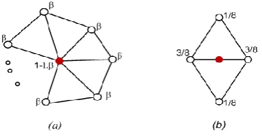
Figure 1. Masks of the Loop subdivision for: (a) vertex-vertices and (b) edge-vertices.
Letting l be the valence of a vertex. The masks for determining the position of a vertex are in Fig.1 [3]. The β weight is a function of l and has been selected such that the limit subdivision surface is smooth [21], it is determined as follows [3]:
2
1 5 3 1 2
cos
8 8 4 and 1
l l l
(1)
Letting i be the number of times of reversing the Loop subdivision. To determine the position of vertices in mesh
Mi-1 from vertices of mesh Mi after reversing the Loop subdivision, we assume that the positions of edge-vertices and vertex-vertices in the Loop subdivision scheme are correlative with weights α and β. Consequently, we have to determine the weights µ and correlative with the weights α and β by using the inverse formulas. Based on the corresponding vertex-vertices pi and their neighbor vertices in mesh Mi, the expression of the inverse vertex-vertices pi-1 in mesh Mi-1 is determined follows:
1 .
1 l
i i i
p p p j
j
(2)
with 5
8 3
and
1
3
8
n
Considering an initial triangular mesh M0(m) with m data points and employing it as a control mesh of a B-patch parametric surface, the degree n of this surface can be determined by the following equation:
1
1 8 3 2
n ( m ) (3)
The triangular B-patch degree will reduce to n/2iafter i steps of the inverse Loop subdivision.
3.2. The B-patch surface
Looking at a region of B-spline on the rectangular domain, B-patch parametric surface on the triangular domain is generalized by assigning knots to the corners of the parametric domain defined for a triangular Bézier surface[4][16]. The collection of knots corresponding to each corner is referred to as a knotcloud (Fig.2).
Figure 2. The triangular parametric domain of a cubic B-patch surface.
For a triangular parametric domain abc, a degree n B-patch surface is defined as follows [16]:
( ) ( )
i j k n V
F u B u p
ijk ijk
(4)where
• The knotvector V = {a0, a1,…, an-1, b0, b1,…, bn-1, c0,
c1,…, cn-1} is associated with the triangular triangular domain abc ≡ a0b0c0, and a0, a1,…, an-1, b0, b1,…, b n-1, c0, c1,…, cn-1R2. Every triple of knots (ai, bj, ck) forms a proper triangle aibjck, with 0 ≤ i+j+k ≤ n-1.
• The polynomials V ( )
Bijk u , with i+j+k=n, is the
normalized B-weight over knotvector V. Letting
ijk,d(u), with d = 0,1,2, are the barycentric coordinates over the domain aibjck. The polynomials BijkV ( )u are
defined recursively as
4 ( ) 1;
000
( ) ( )
1, , ,0 1, ,
( ) , 1, ,1 , 1,
( ) , , 1,2 , , 1
V
B u
V V
B u B u
ijk i j k i j k
V u
i j k i j k
V
B u
i j k i j k
(5)
• The coefficientsp R3
ijk are called control points forming the B-patch control mesh. Letting f be the multiaffine polar form of the polynomial F(u), the B-patch control points are given with blossom label as
0 1 0 1 0 1
( ,..., i , ,..., j , ,..., k )
p f a a
ijk b b c c (6)
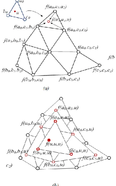
Evaluation, subdivision and differentiation of B-patch surfaces can be computed by using the de Boor-like algorithm [16]. Fig.3a shows a possible configuration of the knotcvectors. A cubic B-patch control mesh and the blending of the top three control points to generate a new point f(a0,a1,u) is shown in Fig.3b.
Figure 3. A cubic B-patch: (a) blending three control points and (b) evaluating B-patch.
The B-patch surfaces can be joined smoothly. The shape of B-patches is strongly influenced by their control meshes and knotvectors. The knot insertion algorithm is also similar
to the insertion one for triangular B-spline. Consequently, the B-patch parametric surfaces inherit some interesting properties of the triangular B-spline surface such as [4], [16]: convex hull property, corner vertex interpolation and tangency at multiple knots, affine invariance, and local control...These properties make B-patch attractive for the interactive smooth surface design.
4. The B-patch surface reconstruction
This section presents a geometric fitting algorithm for approximating the low degree B-patch surfaces over triangular parametric domains from the given triangular meshes.
By using the inverse Loop subdivision scheme, a control polyhedron of a B-patch is generated from the given triangular mesh. And then, this B-patch surface is fitted to data points of the given mesh. In each step of the local geometric fitting algorithm, the control points and knotclouds are also adjusted to minimize the deviation between the data points of the mesh and the reconstructed B-patch surface. The proposed approach can be described by the diagram in Fig. 4.
Figure 4. Flow chart of the proposed approach.
Letting k be the step of the geometric fitting; kj is an error vector corresponding to each data point pj|j=1..mof the given mesh, these vectors are closest distances between the data points of original mesh and their corresponding points on B-patch parametric surface Si; kavg is an average error vector and is computed in each step of the iteration k based on the error vectors kj. Overall steps of the proposed approach can review such as:
5
• The given triangular mesh M0 that is constructed from the m data points pj|j=1..m is set up the data structure in keeping with the Loop subdivision mesh.
• This dense mesh M0 is simplified by using the inverse Loop subdivision scheme. In particular, the edge-vertices are deleted and the vertex-edge-vertices are modified by Eq.(2). The result is that a coarse mesh Mi is obtained after i times of the inverse subdivision.
• Base on Eq.(4), a B-patch surface F is created by employing the obtained mesh Mi as a control polyhedron of the B–patch surface. By this way, the reconstructed surface will have the lower degree comparing to which use the given mesh M0 as a control polyhedron.
• In each fitting step k, the error vectors
kjfor each data point pj of the mesh M0 are also evaluated. These vectors are the closest distances between the data points and their corresponding points on the fitting B-patch surface, and they are determined as follows:k k
j pj F
(7)
with j=1..m and k = 1,2,…
The average error vector k avg
is also computed by the following equation:
1 1 m
k k
avg j
j m
(8)• Base on the average error vector k avg
and the given tolerance , the B-patch is gradually fitted for converging to the data points of the given triangle mesh. In each fitting step k, a triangular fitting mesh
M* is created from m data points * j
p
:* k
j j j
p p (9)
After that, the fitting mesh M* is also simplified by using the inverse Loop subdivision scheme to create a B-patch fitting surface. The knotclouds of the parametric domain and the position of control points are also updated and adjusted in each step of the kth iteration.
In the geometric fitting process, a sequence of the fitting meshes is updated and then simplified, as well as a hierarchy of the fitting B-splines is successively generated after some steps of the iteration in the local fitting algorithm.
The fitting process halts when the average error vector k
avg
is less than the given tolerance . As a result, the reconstructed B-patch is the final obtained surface that passes through most of the data points with the smallest average error. The quality and accuracy of the result surfaces can be carried out by adjusting the knotclouds and changing the position of control points in each of the iteration. The geometric fitting algorithm of the proposed approach for reconstructing B-patch is given in Algorithm 1. In each of the iteration, considering the computation cost of the deviation between each data point and its
corresponding point on the fitting surface is a constant time, with m data points pj, there are m times of computation to be executed correlatively. And supposing that the repeat-until iterates for k times; then the value k depends on the given error tolerance . Consequently, the local geometric fitting algorithm for reconstructing B-Patch surface has an asymptotic complexity
m k ( )
.Algorithm 1. Local geometric fitting algorithm
Input: Triangular mesh M, B-patch Si, error tolerance .
Output: Reconstructed B-patch surface S 1 M0 modiMesh(M)
2 M* M0; k 0 3 Repeat
4 k k+1
5 Mi invSub(M*, i) 6 Di B-patchDomain(Mi) 7 Si B-patchSurf(Mi, Di) 8 for each (pj|j=1..m) do 9 jk errVect(pj, Si) 10 p*j pj + jk 11 end for
12 M* triangularMesh(p*j | j=1..m ) 13 kavgerrAvg(jk)
14 Until (iavg) 15 S Si 16 Return S.
Next, we present convergence of the proposed method. Letting pijl|i+j+l=n be the control points of a degree n B-patch surface over the parametric domain abc, and u be a parameter in the parametric domain abc.
At the beginning of the iteration, k = 0, a B-patch surface
F0(u) is constructed from m=(n+1)(n+2)/2 the control points pijl:
0( ) V( ) 0
ijl ijl i j l n
F u B u p
(10)with pijk0 pijk
Similarly, letting F uk( ) be the B-patch surface
constructed at the kth iteration.
The error vectors are determined as follows:
0 (
k k
ijl pijl F uijl
(11)
So that the control points k1 ijl
p of the B-patch surface
1 ( ) k
F u at the (k+1)th iteration are computed by the following equation:
1
k k k
ijl ijl ijl
p p (12)
And we obtain the B-patch surface 1 ( ) k
F u , that is
6
1 1
( ) ( )
k V k
ijl ijl i j l n
F u B u p
(13)According to Eq.(11), Eq.(11) and Eq.(13), we have
ij
1 0 1
ij 0 1 ij ij i+j+ 0 ij ij i+j+ 0 ij ij i+j+
ij ij ij
i+j+
(
)
(
)
(
)(
)
(
)
(
)
(
)
l k kl ijl ijl
V k
ijl l ijl l
l n
V k k
ijl l ijl l
l n
k V k
ijl ijl l ijl l
l n
k V k
l l ijl l
l n
p
F
u
p
B
u
p
p
B
u
p
p
F u
B
u
B
u
(14)with i+j+l = n and k = 1, 2,…
We can rewrite Eq.(14) in matrix form:
1 1 1
,0,0 1,1,0 0,0,
,0,0 1,1,0 0,0,
...
...
k k k
n n n
k k k
n n n
M
(15)where M = I - B, with I((n+1)(n+2)/2) ((n+1)(n+2)/2) is the identity matrix, and B is the matrix of the polynomials
( ) V
Bijl u over the parametric domain aibjcl
,0,0 ,0,0 1,1,0 ,0,0 0,0, ,0,0
,0,0 1,1,0 1,1,0 1,1,0 0,0, 1,1,0
,0,0 0,0, 1,1,0 0,0, 0,0, 0,0,
(
)
(
)
...
(
)
(
)
(
) ...
(
)
...
...
...
...
(
)
(
)
...
(
)
V V V
n n n n n n
V V V
n n n n n n
V V V
n n n n n n
B
u
B
u
B
u
B
u
B
u
B
u
B
B
u
B
u
B
u
Supposing values
ijl, with i+j+l = n, are (n+1)(n+2)/2eigenvalues of the matrix B. Because the polynomials
( ) V
Bijl u are totally positive, these eigenvalues are all positive. On the other hand, V( ) 1
ijl i j l n
B u
, so the -norms of them B1. Therefore,
0
ijl( ) 1,B i j l nij ij ij
0 1 l( )B l(I B) l(M) 1
, i j l n
This result leads to 0(M)1, with (M)is the spectral radius of the matrix M.
That is, lim k 0,
ijl
k i j l n
equivalently,
lim k( ijl) ijl,
kF u p i j l n (16)
The Eq.(16) shows that the B-patch surfaces k( )
F u converge to the given points pijl after k steps of the iteration.
5. Experimental examples
In this section, we present some experimental results to prove effective of the proposed method. All experiment results in this paper have been obtained on a personal computer with 2.67GHz Intel Core i5 CPU and 4GB RAM. For each example, we consider degree and accuracy of the reconstructed B-patch surfaces, as well as the computational time of the proposed algorithm.
Letting max be the largest deviation of the error vectors
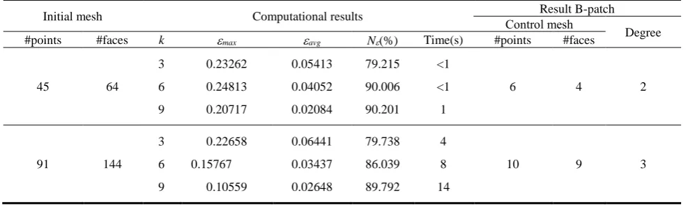
kj; avg be an average deviation between the fitting B-patch and the data points of the given mesh; N(%) is a percent of the number of data points that the obtained B-patch crosses through them. Both the given triangular meshes and reconstructed B-patches of some experimental examples are presented in Table I.
Table 1. Models of test cases
Initial mesh Computational results Result B-patch
Control mesh
Degree #points #faces k max avg N(%) Time(s) #points #faces
45 64
3 6 9 0.23262 0.24813 0.20717 0.05413 0.04052 0.02084 79.215 90.006 90.201 <1 <1 1
6 4 2
91 144
3 6 9 0.22658 0.15767 0.10559 0.06441 0.03437 0.02648 79.738 86.039 89.792 4 8 14
10 9 3
7
153 256
3
6
9
0.38800
0.27048
0.20136
0.04909
0.03894
0.02863
76.848
86.964
90.052 8
16
23
15 16 4
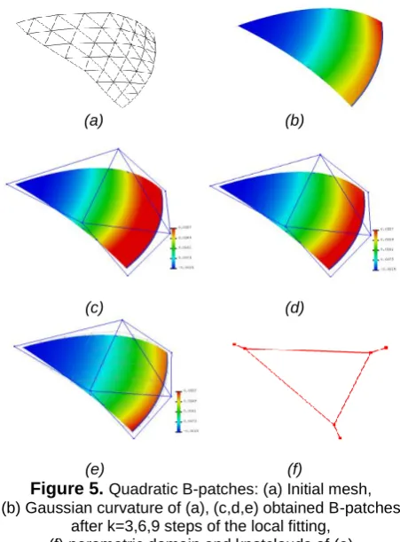
The first example is a quadratic B-patch. Fig.5 illustrates the Gaussian curvatures to compare the quality of the obtained quadratic B-patches with the given mesh. From an initial triangular mesh consisting of 45 points and 64 faces with its curvature image, as shown in Fig.5a and Fig.5b; the quadratic B-patch surfaces can be obtained after i = 2 times of the inverse subdivision and k
= 3, 6, 9 steps of the local geometric fitting, as presented in Fig.5c, 5d, 5e respectively. We can clearly see that a couple of the curvature images in Fig.5b and Fig.5e are rather similar. The images denote that the reconstructed B-patch shape is well approximated to the given mesh. The parametric domain and knotclouds of the obtained B-patch are also illustrated in Fig.5f.
(a) (b)
(c) (d)
(e) (f)
Figure 5.Quadratic B-patches: (a) Initial mesh, (b) Gaussian curvature of (a), (c,d,e) obtained B-patches
after k=3,6,9 steps of the local fitting, (f) parametric domain and knotclouds of (e).
The second and third examples, as cubic and quartic B-patches, are presented in Fig.6. Information on the initial meshes, as well as the details of the reconstructed B-patch surfaces, is listed in Table 1. The triangular meshes of both models in Fig.6a are simplified by using the inverse Loop subdivision scheme.
As a result, we obtained the coarse meshes and employed them as control meshes for creating the cubic
and quartic B-patches. By fitting the position of control points separately with aspect to each error vector, the resulting cubic and quartic B-patches cross through most data points and quickly converge to the given meshes after k = 10 steps of the local geometric fitting (Fig.6b, respectively). The images in Fig.6c are zebra mapping of the reconstructed cubic and quartic B-patches with k = 10, and their parametric domains along with knotclouds are also presented in Fig.6d.
(a)
(b)
(c)
(d)
Figure 6.Cubic (left) and quartic (right) B-patches: (a) Initial mesh, (b) obtained B-patches and their control
meshes after k = 10 steps of the local fitting, (c) zebra mapping of (b), (d) parametric domains
and knotclouds of (b).
Table 1 also presents that the low-value max and avg, while the rather high-value N corresponding to the number of iteration k. The execution times is also proportional to the degree of the result B-patch surfaces as well as the number of iteration k.
Finally, to prove of the accuracy of the obtained low degree B-patches can be carried out by adjusting the control mesh in each step of the iteration k, we illustrate
8 plots of both values values avg and N in Fig.7 and Fig.8. The average error measures avg sharply decrease in the first three iterations and then gradually decay to range from 0.004 to 0.006 in Fig.7. In contrast, the values N
rapidly increase in the first three iterations, and after that, they reach to range from 90% to 95%, as shown in Fig.8. The plots indicate that the values avg and N depend on the number of iterations k; consequently, the reconstructed B-patch surfaces can be obtained after several steps k of the local geometric fitting algorithm.
Figure 7. Average errors with respect to the number of iteration k.
Figure 8.Convergence are proportional to the number of iteration k.
5. Conclusions
In this paper, we have proposed a new method for reconstructing the low degree B-patch parametric surfaces from the triangular meshes based on the inverse subdivision scheme along with the local geometric fitting algorithm; particularly, they are the quadratic, cubic and quartic B-patches over the triangular parametric domain. By using the inverse Loop subdivision scheme to simplify the given triangular mesh and applying the local
geometric fitting algorithm to adjust the control points of a B-patch, a sequence of the B-patch surfaces is generated after k steps of the iteration. As a result, the obtained B-patch surface well approximates the data points of the initial mesh. Our approach has the following features:
•Avoiding the shortcomings of the least-square fitting method and linear system solution, the reconstructed B-patches still cross through most data points of the initial mesh after several steps of the iterations.
•By using the inverse subdivision scheme to simplify the control mesh, the degree of the result B-patches will be reduced to 2i times after i steps of the reversing subdivision.
•The accuracy of the obtained B-patch surfaces can be carried out by changing the position of control points in the local geometric algorithm.
Because most surfaces often employed in geometric design are the low degree patches, especially the cubic patches, this result has practical significance for geometric design, data compression, surface editing and manipulation, versatile design, especially for reverse engineering and virtual reality.
References
[1] Deng, C. and Lin, H. (2014) Progressive and iterative approximation for least squares B-spline curve and surface fitting. Computer-Aided Design 47: 32–44.
[2] Deng, C. and Ma, W. (2012) Weighted progressive interpolation of Loop subdivision surfaces. Computer-Aided Design 44: 424–31.
[3] Loop, C. (1987) Smooth Subdivision Surfaces Based on Triangles. M.S. Mathematics thesis.
[4] Ingram, C.K. (2003) Geometric B-Spline Over the Triangular Domain. M.S.Mathematics thesis.
[5] Zorin, D. and Schroder, P. (2000) Subdivision for Modeling and Animation. SIGGRAPH Course Notes. [6] Pratiwi, D. (2013) The Implementation of Univariate and
Bivariate B-Spline Interpolation Method in Continuous.
IJCSI International Journal of Computer Science 10(2). [7] Cheng, F. and et al. (2009) Loop subdivision surface based
progressive interpolation. Journal of Computer Science and Technology 24: 39–46.
[8] Farin, G. (2002) Curves and Surfaces for Computer Aided Geometric Design: A Practical Guide, 5th ed. (Morgan Kaufmann: San Mateo).
[9] Greiner, G. (2010) Geometric modeling. Lecture in Winter Term.
[10] Chen, J. and Wang, G. (2011) Progressive iterative approximation for triangular Bézier surfaces. Computer-Aided Design 43: 889–895.
[11] Eck, M. and Hoppe, H. (1996) Automatic reconstruction of B-spline surfaces of arbitrary topological type. In Proceedings of SIGGRAPH96 (ACM Press), 325–334. [12] Botsch, M. and et al. (2006) Geometric Modeling Based on
Triangle Meshes. EuroGraphics.
[13] Neamtu, M. (2001) Bivariate simplex B-splines: a new paradigm. In Proceedings of the 17 th spring conference on computer graphics, 71–78.
9 [14] Nga, L.T.T, Khoi N.T. and Thuy, N.T. (2014)
Reconstructing low degree triangular parametric surfaces based on inverse Loop subdivision. In Proceedings of the International Conference on Nature of Computation and Communication 144: 98-107.
[15] Cheng, S. and et al. (2012) Delaunay Mesh Generation.
Computer & Information Science Series (CRC Press). [16] Seidel, H.P. (1991) Symmetric recursive algorithms for
surfaces: b-patches and the de Boor algorithm for polynomials over triangles. Constructive Approximation 7: 257–279.
[17] Maekawa, T. and et al. (2007) Interpolation by geometric algorithm. Computer-Aided Design 39:313–323.
[18] Kineri, Y. and et al. (2012) B-spline surface fitting by iterative geometric interpolation/approximation algorithms.
CAD 44(7): 697–708.
[19] Nishiyama, Y. and et al. (2008) Loop subdivision surface fitting by geometric algorithms. In proceedings of pacific graphics.
[20] Xiong, Y. and et al. (2012) Convergence analysis for B-spline geometric interpolation. Computers & Graphics
36:884–891.
[21] Zhao, Y. and Lin, H. (2011) The PIA property of low degree non-uniform triangular B-B patches. In Proceedings of the 12th International Conference on CAD and CG, 239-243.