Opinion Broadcasting Model

University of Pennsylvania

ScholarlyCommons

Publicly Accessible Penn Dissertations

2018

Opinion Broadcasting Model

Chenchao Chen

University of Pennsylvania, [email protected]

Follow this and additional works at:https://repository.upenn.edu/edissertations Part of theMathematics Commons

This paper is posted at ScholarlyCommons.https://repository.upenn.edu/edissertations/3062

For more information, please [email protected]. Recommended Citation

Chen, Chenchao, "Opinion Broadcasting Model" (2018).Publicly Accessible Penn Dissertations. 3062.

Opinion Broadcasting Model

Abstract

Stochastic approximation methods have been widely used in random processes with reinforcement. Applications include root approximation algorithm, interacting urn models, and continuous reinforced processes. Emphasis is on the establishment of a so-called opinion broadcasting model, with the proof of an asymptotic result for such process using the idea of some stochastic approximation method.

Degree Type

Dissertation

Degree Name

Doctor of Philosophy (PhD)

Graduate Group

Mathematics

First Advisor

Robin Pemantle

Subject Categories

OPINION BROADCASTING MODEL

Chenchao Chen

A DISSERTATION

in

Mathematics

Presented to the Faculties of the University of Pennsylvania in Partial

Fulfillment of the Requirements for the Degree of Doctor of Philosophy

2018

Supervisor of Dissertation

Robin Pemantle, Professor of Mathematics

Graduate Group Chairperson

Wolfgang Ziller, Professor of Mathematics

Dissertation Committee:

Robin Pemantle, Professor of Mathematics

J. Michael Steele, Professor of Statistics

Acknowledgments

Firstly, I would like to express my sincere gratitude to my advisor Prof. Robin

Pemantle for the continuous support of my Ph.D study and related research, for

his patience, motivation, and immense knowledge. His guidance helped me in all

the time of research and writing of this thesis. I could not have imagined having a

better advisor and mentor for my Ph.D study.

Besides my advisor, I would like to thank the rest of my thesis committee:

Prof. J. Michael Steele and Prof. Greta Panova, for their insightful comments

and encouragement, but also for the hard question which incented me to widen my

research from various perspectives.

I thank my fellow Ph.D colleague Konstantinos Karatapanis for the stimulating

discussions, for very careful review of my draft papers, and for all the valuable ideas

and suggestions on my project. Also I thank my friends in math department for

the time I spent here.

Last but not the least, I would like to thank my parents for supporting me

ABSTRACT

OPINION BROADCASTING MODEL

Chenchao Chen

Robin Pemantle

Stochastic approximation methods have been widely used in random processes with

reinforcement. Applications include root approximation algorithm, interacting urn

models and continuous reinforced processes. Emphasis is on the establishment of

a so-called opinion broadcasting model, with the proof of an asymptotic result for

Contents

1 Introduction 1

2 Background 3

2.1 Root approximation model . . . 4

2.2 Urn models . . . 6

2.3 Dynamic systems . . . 8

3 Opinion propagation model 11

3.1 Main results . . . 12

3.2 Further conjectures . . . 14

4 Proof of theorem 3.1.3 16

4.1 Basic Construction and Proof Outline . . . 16

4.2 Proof of I . . . 22

Chapter 1

Introduction

The Random process with Reinforcement has grown substantially within the past

twenty years. In some sense, it is still a collection of disjoint techniques. The few

difficult open problems that have been solved have not led to broad theoretical

advances. On the other hand, some nontrivial mathematics is being put to use in a

fairly coherent way by communities of social and biological scientists. As a result,

several useful techniques are introduced, among which, the stochastic approximation

/ dynamical system approach and the multitype branching process approach could

be called theories which contain their own terminology, constructions, fundamental

results, compelling open problems and so forth. However, the later one pioneered

by Athreya and Karlin has been taken pretty much to completion by the work of

S. Janson.

reinforce-ment in continuous time and space. Continuous reinforcereinforce-ment processes are to

reinforced random walks what Brownian motion is to simple random walk, that is

to say, there are new layers of complexity. There are several self-interacting

dif-fusions and more general continuous-time processes that open up mathematics of

some depth and practical relevance.

Opinion propagation model is a particular example fit into the catagory of

ran-dom process with reinforcement, which originally comes from one of Elchanan

Mos-sel’s former students. This resulting paper will study a special case of this model

using stochastic approximation / dynamic system via martingale methods. There

are some potential open questions relavant to this model which either requires more

delicate analysis or encounters new form of stochastic approximation.

The organization of the rest of the paper is as follows. Chapter 2 provides

an overview of stochastic approximation methods, dynamic system approach and

their applications. Chapter 3 introduces the opinion broadcasting model and its

motivation, listing the main result and further conjectures. Chapter 4 is devoted

Chapter 2

Background

The purpose of this chapter is to introduce the stochastic approximation process,

dynamic system approach and several of their applications. Because of the way

research has developed, the existing theoretical results are very much tailored to

speific applications and are not easily discussed abstractly. We start with the root

approximation model in chapter 2.1 where the stochastic approximation method

first introduced. We further look at its applications in urn models in chapter 2.2.

Finally, chapter 2.3 is about the dynamical systems and their stochastic

2.1

Root approximation model

In [RM51], the stochastic approximation process was first introduced by Herbert

Robbins and Sutton Monro. They used this to approximate the root of an unknown

function in the setting where evaluation queries may be made but the answers are

noisy.

To be more specific, let M(x) be a given function and α a given constant such

that the equation

M(x) = α (2.1.1)

has unique root x = θ. There are many methods for determining the value of θ

by successive approximation (root-finding algorithm). With any such method we

begin by choosing one or more values x1,· · · , xr more or less arbitrarily, and then

successively obtain new values xn as certain functions of the previously obtained

x1,· · · , xn−1, the values M(x1),· · · , M(xn−1) and possibly those of the derivatives

M0(x1),· · · , M 0

(xn−1), etc. If

lim

n→∞xn=θ, (2.1.2)

irrespective of the arbitrary initial values x1,· · · , xr, then the method is effective

for the particular function M(x) and value α.

The stochastic generalization of the above problem in which the nature of the

variable Y =Y(x) with distributionP(Y(x)≤y) =H(y|x) such that

M(x) =

Z ∞

−∞

ydH(y|x)

is the expected value ofY for the givenx. NeitherH(y|x) nor M(x) is known here,

but it is assumed that equation (2.1.1) has a unique root θ, and it is desired to

estimate θ by making successive observations on Y at levels x1, x2,· · · determined

sequentially in accordance with some definite experimental procedure. [RM51] gives

a particular procedure for estimatingθ which is consistent under certain restrictions

on the nature of H(y|x) where the consistency is in the sense that (2.1.2) holds in

probability irrespective of any arbitrary initial values x1,· · · , xr.

In the proofs, they defined a fixed sequence{an}of positive constants such that

0<X

n

a2_n=A <∞.

Furthermore, they defined a Markov chain {xn} by taking x1 to be an arbitrary

constant and defining

xn+1−xn =an(α−yn), (2.1.3)

where yn is a random variable such that

P(yn≤y|xn) =H(y|xn).

A natural candidate for an can be an= _n1, then (2.1.3) becomes

xn+1−xn=

1

where yn∈ Fn. (2.1.4) is an example of a stochastic approximation process.

More generally, let {Xn :n ≥0} be a stochastic process in the euclidean space

Rd _{and adapted to a filtration{F}

n}. Suppose thatXn satisfies

Xn+1−Xn=

1

n(F(Xn) +ξn+1+Rn) (2.1.5)

where F is a vector field on Rd_{, E(ξ}

n+1|Fn) = 0 and the remainder terms Rn∈ Fn

go to zero and satisfy P∞

n=1n

−1_|R

n| < ∞ almost surely. Such a process is known

as a stochastic approximation process.

2.2

Urn models

The original P´olya urn model which first appeared in [EP23] has an urn that begins

with one red ball and one black ball. At each time step, a ball is chosen at random

and put back in the urn along with one extra ball of the color drawn, this process

being repeated infinitely many times. We construct this recursively: let R0 = a

and B0 = b for some constants a, b > 0; for n ≥ 1, let Rn+1 = Rn +1Un+1≤Xn

and Bn+1 = Bn+1Un+1>Xn, where Xn := Rn/(Rn+Bn). We interpret Rn as the

number of red balls in the urn at time n and Bn as the number of black balls at

time n. Uniform drawing corresponds to drawing a red ball with probability Xn

independent of the past; this probability is generated by oursource of randomness

via the random variable Un+1, with the event {Un+1 ≤ Xn} being the event of

Later, P´olya’s urn has been generalized by taking the number of colors to be

any integer k ≥ 2. The number of balls of color j at time n will be denoted Rnj.

Secondly, fix real numbers {Aij : 1 ≤ i, j ≤ k} satisfying Aij ≥ −δij where δij

is the Kronecker delta function. When a ball of color i is drawn, it is replaced

in the urn along with Aij balls of color j for 1 ≤ j ≤ k. The reason to allow

Aii ∈ [−1,0] is that we may think of not replacing (or not entirely replacing) the

ball that is drawn. Formally, the evolution of the vector Rn is defined by letting

Xn := Rn/

Pk

j=1Rnj and setting Rn+1,j = Rnj +Aij for the unique i satisfying

P

t<iXnt < Un+1 ≤

P

t≤iXnt. This guarantees that Rn+1,j = Rnj + Aij with

probability Xni for eachi. We call this model generalized P´olya urn scheme (GPU)

where the reinforcement is Aij.

To relate between stochastic approximations and urn processes, we denote by

Qn, the probability distributions governing the color of the next ball chosen which

are typically defined to depend on the content vector Rn only via its normalization

Xn. Ifb new balls are added toN existing balls, the resulting incrementXn+1−Xn

is exactly b

b+N(Yn−Xn) where Yn is the normalizedvector of added balls. Since b

is of constant order and N is of ordern, the mean increment is

E(Xn+1−Xn|Fn) =

1

n(F((Xn) +O(n

−1₎₎

where F(Xn) =b·(E(Yn|Fn)−Xn). Defining ξn+1 to be the martingale increment

Xn+1−E(Xn+1|Fn) recovers (2.1.5).

nonconvergence to unstable equilibria [Pem88] are based on this stochastic

approx-imation form of GPU.

2.3

Dynamic systems

In terms of [Ben99], Bena¨ım and collaborators have formulated an approach to

stochastic approximations based on notions of stability for the approximating ODE.

Here we briefly describe the dynamical system approach.

For processes in any dimension obeying the stochastic approximation equation

(2.1.5), there are two natural heuristics. Sending the noise and remainder terms

to zero yields a difference equation Xn+1 −Xn = n−1F(Xn) and approximating

Pn

k=1k

−1 _{by continous variable logt yields the differential equation}

dX

dt =F(X). (2.3.1)

The first heuristic is that trajectories of the stochastic approximation {Xn} should

approximate trajectories of the ODE {X(t)}. The second is that stable trajectories

of the ODE should show up in the stochastic system, but unstable trajectories

should not.

The whole rigorous theory hugely relied on some pure topological concepts which

I will omit here. Instead, I will include those results related to probabilistic analysis

from [Ben99].

[BH96], is the asymptotic pseudotrajectory.

Definition 2.3.1 (asymptotic pseudotrajectories). Let (t, x)7→Φt(x) be a flow on

a metric space M. For a continuous trajectory X :R+ _{→M, let}

dΦ,t,T := sup 0≤h≤T

d(X(t+h),Φh(X(t)))

denote the greatest divergence over the time interval [t, t+T] between X and the

flow Φ started from X(t). The trajectory X is an asymptotic pseudotrajectory for

Φ if

lim

t→∞dΦ,t,T(X) = 0

for all T >0.

Turning to the first convergence heuristic, from [Ben99] Proposition 4.4 and

Theorem 7.3, we have:

Theorem 2.3.2 (stochastic approximations are asymptotic pseudotrajectories).

Let {Xn}be a stochastic approximation process, that is, a process satisfying(2.1.5),

and assumeF is Lipschitz. Let {X(t) :=Xn+(t−n)(Xn+1−Xn) for n≤t < n+1}

linearly interpolate X at nonintegral times. Assume bounded noise: |ξn| ≤K. Then

{X(t)} is almost surely an asymptotic pseudotrajectory for the flow Φ of integral

curves of F.

Theorem 2.3.3 (convergence to an attractor). Let A be an attractor for the flow

approximation X := {Xn}. Then either (i) there is a t for which {Xt+s : s ≥ 0}

almost surely avoids some neighborhood of A or (ii) there is a positive probability

that L(X)⊆A.

For the nonconvergence heuristic, most known results are proved under linear

instability. This is a stronger hypothesis than topological instability, requiring that

at least one eigenvalue ofdF have strictly positive real part. From [Ben99] Theorem

9.1, we have:

Theorem 2.3.4(nonconvergence under linear instability). Let{Xn}be a stochastic

approximation process on a compact manifold M with bounded noise |ξn| ≤ K for

alln andC2 _{vector field F. LetΓbe a linearly unstable equilibrium or periodic orbit}

for the flow induced by F. Then

P( lim

Chapter 3

Opinion propagation model

The opinion propagation model is a general model on any graph that originally

comes from one of Elchanan Mossel’s former students. Let G be a finite

con-nected graph; the nodes represent people and the edges represent that they interact.

Choose an integer k ≥ 2, the set [k] is interpreted as a set of k different opinions,

say possible names for a baby, on which it is desired to form a consensus. The

states of the system are maps ξ : V(G) → 2[k]_{, in other words every person}

sub-scribes to some subset of all possible opinions. Maps for whichξ(v) is empty set for

some v are not allowed. The problem is to study after exchanging information for

how many times (or how long in the continuous version) will the state terminates

in consensus. in order words after how much time of discussion will every person

agrees of a certain name for the baby.

one of their opinions, and independently chooses a uniform neighbor w. Suppose

j ∈ [k] and w ∈ V(G) are chosen. If j /∈ ξ(w) then the new state ξ0 agrees with ξ

away from w but has ξ0(w) =ξ(w)∪ {j}. If alreadyj ∈ξ(w) thenξ0 agrees with ξ

except at the two sites v and w, resetting ξ0(v) =ξ0(w) ={j}. The interpretation

is: if you hear a new name you add it to your list; if you hear one you already have

in mind, then immediately you and the person you heard it from coordinate on the

new name and forget all other names.

3.1

Main results

There is only one thing known for this model:

Theorem 3.1.1. If G = KN, the complete graph on N vertices, and k = 2 (two

possible opinions), then starting from any configuration, the state terminates in

consensus in Θ(NlogN) steps.

In the rest of the paper, we will improve the result of the above theorem by

replacing Θ(·) with deterministic coefficients for the leading terms. Before listing

the main result, we need some notations, basic constructions of them, and some

definitions as preparation.

When k = 2, we denote the two opinions as opinion A and opinion B. Hence

at any time there are at most three types of opinions: {A}, {B}, and {A, B}. We

and {A, B} respectively at time t. Obviously we have XN

t +YtN +ZtN = 1 for all

t ≥0.

Next, we give the following definitions with respect to the area spanned by

(X, Y, Z)t’s:

Definition 3.1.2. We denote T :={(X, Y, Z) : 0≤X, Y, Z ≤1, X +Y +Z = 1},

and we specify the subset our initial configuration locates as SInter := {(X, Y, Z) :

X, Y, Z ≥20,|X−Y| ≥ 20, X+Y +Z = 1} for arbitrary small constant 0 >0.

Furthermore, we define Slog−dist := {(X, Y, Z) : Y2 +Z2 ≤ log

−2

N, Y2 +Z2/4 >

1/N2_{, X +Y +Z = 1} ∪ {(X, Y, Z) : X}2_+Z2 _≤log−2

N, X2_+Z2_/4>1/N2_{, X +}

Y +Z = 1} and SD := {(X, Y, Z) : (1,0,0),(1− _N1,_N1,0),(1− _N1,0,_N1),(_N1,1−

1

N,0),(0,1− 1 N,

1

N),(1− 2 N,0,

2

N),(0,1− 2 N,

2

N),(0,1,0)} which will be used in later

proof.

(1,0,0) X S_Inter

(0,0,1) Z (0,1,0)

Y

_{Barycentric Coordinate}

Slog

log

S

Inter

S SD

S_D

Now we are ready to state our main theorem:

Theorem 3.1.3. If G = KN, and k = 2, let τ := inf{t : (XN, YN, ZN)t =

(1,0,0)or (0,1,0)}. Then, for any starting point (XN, YN, ZN)0 ∈ SInter, τ =

logN + log logN +o(log logN) in probability as N → ∞.

3.2

Further conjectures

Here we list two conjectures which may worth further discussions.

• Theorem 3.1.3 claims that τ is logN + log logN +o(log logN), while we

fur-ther conjecture the exact asymptotic form is possibly logN+ log logN+O(1)

• In theorem 3.1.3, we gave an asymptotic expression of the stopping time with

initial configuration restricted to SInter. Further work may be focusing on the

initials (1) near the boundary: (x0, y0, z0)→ ∂T, in such case we conjecture

the time is of the form logN+O(1) without the log logN term; (2) near the

center: |x0−y0| → 0, where we conjecture the form c∗logN +o(logN) with

Chapter 4

Proof of theorem 3.1.3

4.1

Basic Construction and Proof Outline

First, following [Fox16], we give definitions for drift and variance for general pure

jump markov process.

Definition 4.1.1. Let{X}t be a pure jump markov process defined on some

com-pact set K ⊂ Rd _{adapted to filtration {F}

t : t ≥ 0}. The total jump rate at time

t is denoted as qt which we assume is uniformly bounded. Then, there exists a

probability measure νt on K s.t.

lim

h→0P(Xt has a jump in [t, t+h] by vector in A|Ft)·h

−1 _=q

We define the jump forX to be ∆Xt :=Xt−Xt− at timet, then define

µt(X) = qt

Z

∆Xtdνt(∆Xt)

Σt(X) = qt

Z

∆Xt·∆XTtdνt(∆Xt),

to be the drift vector and covariance matrix for {X}t respectively.

Now using the notations we mentioned in the previous section, we construct

the formulas for both drift and coordinate variance for the (XN_{, Y}N_{, Z}N₎

t process.

Here the coordinate variance is just three variance terms in ΣN_t , i.e. (ΣN₁₁,ΣN₂₂,ΣN₃₃)T

which we denote as σN2

t for convenience. For the rest covariance terms, we will see

that ΣN

12 = ΣN21 is the only one needed in the later proofs, so we will derive the

formula for it as well.

First, we note the jump rate for broadcasting one opinion for the whole

sys-tem {XN_{, Y}N_{, Z}N_}

t equals to N for any t ≥ 0 since each person independently

broadcasts an opinion at rate 1.

For the drift, according to the assumption of the rules for broadcasting, we have

{A} {B} {A, B}

{A} ({A}, {A}) ({A}, {A,B}) ({A}, {A})

{B} ({B}, {A, B}) ({B}, {B}) ({B}, {B})

{A, B} 1

2({A},{A}) 1

2({A, B},{A, B}) 1

2({A},{A})

{A, B} 1

2({A, B},{A, B}) 1

2({B},{B}) 1

2({B},{B})

Table 4.1: Possible Changes of Opinions after Broadcasting

where the first column represents the opinion state for the person who is to broadcast

his opinion, while the first row represents the opinion state for the person who is

to receive opinion. Furthermore, the fourth row represents the resulting opinon set

of both deliverer and receiver given the deliverer choosing to broadcast opinion A,

while choosing to broadcast B in the fifth row. The 1₂ factor in the last two rows

means half-and-half probability for the resulting opinion set given the deliverer

holding {A, B}.

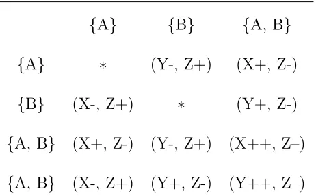
We can transfer table 4.1 into the table of changes of (XN, YN, ZN)t:

{A} {B} {A, B}

{A} ∗ (Y-, Z+) (X+, Z-)

{B} (X-, Z+) ∗ (Y+, Z-)

{A, B} (X+, Z-) (Y-, Z+) (X++, Z–)

{A, B} (X-, Z+) (Y+, Z-) (Y++, Z–)

where∗means no change, ·+ = ·+_N1,·−=· − 1

N,·+ + =·+ 2

N, and· − −=· −

2 N.

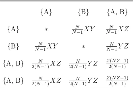
Next, we compute the probability for all possibilities of the changes in (XN, YN, ZN),

and it follows table 4.3 as below:

{A} {B} {A, B}

{A} ∗ N

N−1XY N N−1XZ

{B} N

N−1XY ∗

N N−1Y Z

{A, B} N

2(N−1)XZ N 2(N−1)Y Z

Z(N Z−1) 2(N−1)

{A, B} N

2(N−1)XZ N 2(N−1)Y Z

Z(N Z−1) 2(N−1)

Table 4.3: Probability for all Possible Changes

For example, the probability that deliverer holds {A}, and the receiver holds {B}

has probability X · N Y

N−1 = N

N−1XY given the current proportion vector being

{X, Y, Z}. The rest probabilities can be similarly derived in table 4.3.

Therefore, according to definition 4.1.1, the drift for XN

t equals to

N · 1

N ·( N

N −1(XZ−XY +Z

2₎₋ Z

N −1) =

N

N −1(XZ −XY +Z

2₎₋ Z

N −1,

which asymptotically equals to (XNZN −XNYN +ZN2)t asN → ∞. Here in the

first expression, the N term is the rate for broadcasting of the system, the _N1 term

is the unit change of XN

t , and the rest is the probability of different changes ofXtN.

drift vector µN

t for (XN, YN, ZN)t equals to:

(XZ −XY +Z2, Y Z−XY +Z2,2XY −XZ−Y Z−2Z2)·(1 +O(1

N)).

(4.1.1)

Secondly, we can also compute the coordinate variance according to definition

4.1.1, table 4.2, and table 4.3. In particular, the variance for XN

t equals to

N· 1 N2((

N

N −1(XZ+XY+XZ+2Z

2₎₋ 2Z

N −1) =

1

N −1(XY+2XZ+2Z

2₎₋ 2Z

N(N −1),

where in the first expression theN term again represents the time rate for changing,

the _N12 is the square of unit change ofX_tN, and the rest is the probability of different

changes of XN

t .

Similarly, we have formulas of coordinate variances for Y_tN and Z_tN, whence we

have the coordinate variance vector σN2

t for (XN, YN, ZN)t equals to:

1

N(XY + 2XZ + 2Z

2_{, XY + 2Y Z+ 2Z}2_{,2XY + 2Y Z+ 2XZ+Z}2_{)·(1 +O(}1

N)).

(4.1.2)

Finally, we come to the covariance for X_tN and Y_tN. Since we observe that it is

impossible for both X and Y to change values at the same time, so the covariance

for them equals to 0, i.e. ΣN

12 = 0.

According to [Kur77], the pure jump markov process (XN, YN, ZN)t converges

satisfying

d(X, Y, Z)t =µt(X, Y, Z)dt,

µt(X, Y, Z) = (XZ−XY +Z2, Y Z −XY +Z2,2XY −XZ −Y Z −2Z2)t.

(4.1.3)

Furthermore, [Kur77] also showed in probability that

sup

t≤T

|(XN, YN, ZN)t−(X, Y, Z)t| ≤(|(XN, YN, ZN)0−(X, Y, Z)0|+

C1

√ N)e

C2T

(4.1.4)

for some constants C1, C2 >0 independent ofN and arbitraryT > 0, which we will

be using repeatedly in chapter 4.2.

Therefore, our idea is to approximate this pure jump markov process by this

de-terministic model when the process is away from the two termination states (1,0,0)

and (0,1,0), whereas instead of diffusion, we will use Poisson process and

stochas-tic approximation via martingale methods to estimate the time when the process is

approaching the termination points.

We prove theorem 3.1.3 by seperating the procedure into two parts. Note that

X and Y are symmetric in terms of termination, WLOG, we assume the starting

point is in the half region wherex0 > y0 insideSInterfor the rest sections.The outline

of the proof is as follows:

I Given the starting point v0 ∈ SInter, denote τIenter := inf{t : (XN, YN, ZN)t ∈

II Given the starting pointv0 ∈∂Slog−dist, denoteτlog := inf{t: (XN, YN, ZN)t∈

SD}, then τlog = logN +o(log logN) in probability;

III It takes O(1) for any pointv0 ∈SD to reach absorbing point.

In particular, we will prove I in chapter 4.2; prove II and III as well as completion

of proof for the theorem in chapter 4.3.

4.2

Proof of I

First, before proving I, recall that we obtain the drift vector (4.1.3) for the

corre-sponding determinisitc model in chapter 4.1, since here we focus ourselves to the

case where x0 −y0 ≥ 20 which is straightforwardly depending on the process for

{Y_tN, Z_tN}, basically we will be using both terms forY_tN and Z_tN. Furthermore, we

can rewrite them in terms of Y, Z using the equationX+Y +Z = 1. Namely,

µt(Y, Z) = (Y Z−XY +Z2,2XY −XZ−Y Z −2Z2)t

= (Y Z−(1−Y −Z)Y +Z2,(1−Y −Z)(2Y −Z)−Y Z −2Z2)t

= (−Y + (Y +Z)2,2Y −Z−Y2 −(Y +Z)2)t, (4.2.1)

we will be using drift in either form (4.1.3) or (4.2.1) when necessary.

In order to show τInter = log logN +o(log logN) in probability, it is equivalent to

show that: ∀δ >0, we have

The outline to verify the above inequalities is as following:

1. ∃L(δ), 1(δ), 2(δ) > 0 such that YLN ≤ 2δZ N

L and 1(δ) ≤ YLN, ZLN ≤ 2(δ) in

probability;

2. YN

t ≤δZtN in probability for L≤t≤τInter, and we derive (4.2.2).

We verify the first statement using lemma 4.2.1-4.2.2.

Lemma 4.2.1. Suppose we start at (x0, y0, z0) ∈ SInter satisfying x0 −y0 ≥ 20,

then ∃L(∗) s.t.

P(∗∗≤Y_LN, Z_LN ≤∗)→1 as N → ∞,

for arbitrary ∗ >0 and ∗∗>0 depending on ∗.

Proof. It is sufficient to show for some L(∗)

∗∗≤YL, ZL≤∗

for the corresponding deterministic process due to (4.1.4) and (X0, Y0, Z0) = (x0, y0, z0).

First, we define Ut=Xt−Yt. Then U0 ≥20.

According to (4.1.3), the drift ofUtequals toZtUtwhich is non-negative.

Second, letVt= (2 +0)Yt+Zt, according to (4.2.1), we have

µ(Vt) = −(2 +0)Yt+ (2 +0)(Yt+Zt)2+ 2Yt−Zt−Yt2−(Yt+Zt)2

=−0Yt+0Yt2 −Zt(1−2(1 +0)Yt−(1 +0)Zt)

=−0Yt(1−Yt)−Zt(Xt−Yt−0(1−Xt+Yt))

≤ −(1

2+0)0Yt−0Zt

≤ −0

4Vt.

On the other hand, solving the following differential equation:

dV0 =−0 4V

0

dt, V₀0 =V0 = (2 +0)y0+z0

gives us

V_t0 =V0e−

₀t

4 .

Therefore, by letting t0 = 4−01(logV0−log∗), we have

V_t0₀ =∗

which indicates

Vt0 ≤

∗

.

Note that Vt0 = (2 +0)Yt0 +Zt0 ≤

∗ _{implies bothY}

t0 and Zt0 are smaller than

∗_.

Third, we complete the proof by showing both Yt0 and Zt0 are greater than

In terms of (4.2.1), we have the following inequalities for µ(Y) and µ(Z):

µ(Y)≥ −Y;

µ(Z)≥ −2Z.

Therefore, the two following ODE’s

dY0 =−Y0dt, Y₀0 =y0;

dZ0 =−2Z0dt, Z₀0 =z0

derives Y_t0 =y0e−t and Z 0

t =z0e−2t.

If we let ∗∗= 20e−2t0, then

Yt0 ≥

∗∗

,

Zt0 ≥

∗∗

,

here we use the assumption that Y0, Z0 ≥20.

In sum, letL(∗) =t0, we conclude

∗∗≤YL, ZL≤∗

for arbitrary ∗ >0, whence

P(∗∗ ≤Y_LN, Z_LN ≤∗)→1 as N → ∞,

we are done.

Lemma 4.2.2. Suppose we start at (x0, y0, z0) such that ∗∗(δ) ≤ y0, z0 ≤ ∗(δ),

then ∃L, T(δ), L≤T(δ) s.t.

Y_LN ≤ δ 2Z

N

where ∗ = ₁₆₍₁₊₂δ _/δ)2 and

∗∗ _{depends on} ∗ _{in terms of lemma 4.2.1.}

Proof. As similar to lemma 4.2.1, it is sufficient to show

YL ≤

δ

2ZL for some L≤T(δ)

for the corresponding deterministic model because of (4.1.4) andT(δ) not depending

on N.

First, from the proof in lemma 4.2.1, we seeVt = (2+0)Yt+Ztis non-increasing.

Therefore, Vt≤V0 ≤4∗ which implies Yt, Zt≤4∗ for all t.

Second, we define τ := inf{t : δ₂Zt−Yt ≥ 0}. If y0 ≤ δ₂z0, then we are done.

Otherwise, we have y0 > δ₂z0. Therefore, ∀t < τ, we have

µ(Y)≤ −Y + (1 + 2/δ)2Y2

≤ −(1−4(1 + 2/δ)2∗)Y;

µ(Z)≥δZ −Z−(δ2/4 + (1 +δ/2)2)Z2

≥ −(1−δ+ 4(δ2/4 + (1 +δ/2)2)∗)Z.

Furthermore, if we plug in ∗ = ₁₆₍₁₊₂δ_/δ)2, we deduce

µ(Y)≤ −(1−δ/4)Y;

µ(Z)≥ −(1−δ/2)Z.

Therefore, we have the following inequalities:

Yt≤y0e−(1−δ/4)t;

Let t0 = 4_δlog ∗

δ∗∗, then we have Yt0 ≤

δ 2Zt0.

Finally, let T(δ) =t0, we haveτ ≤T(δ). Thus, we are done with the proof.

Next, we verify the second statement using lemma 4.2.3-4.2.4. Before we go

ahead, from lemma 4.2.2, we see that ∃Lindependent of N (in fact,L≤ 4

δlog ∗ δ∗∗)

such thatYL≤ δ₂ZL, and bothYLandZLare bounded between two positive numbers

independent of N (in fact, the one candidate for upper bound is 4∗ = ₄₍₁₊₂δ_/δ)2).

We denote 3 and 4 as the lower and upper bounds for YL and ZL respectively for

the later proof.

Lemma 4.2.3. Suppose we start at (x0, y0, z0)such that y0 ≤ δ₂z0 and 3 ≤y0, z0 ≤

4, then

Y_tN ≤δZ_tN ∀t <2 log logN in probability.

Proof. First, let T = 2 log logN in (4.1.4), we have

sup

t≤2 log logN

|(XN, YN, ZN)t−(X, Y, Z)t| ≤

C1

√

Ne

C2log logN

= C1log

C2_N

√ N

log−1N in probability. (4.2.3)

We will be using (4.2.3) later in this proof.

Second, from lemma 4.2.2, we see 2Yt+Zt ≤ 44 for all t. let Wt = δZt−Yt,

then W0 =δz0−y0 ≥y0 ≥3.

We claim: ∃θ(δ)>0 s.t.

which is equivalent to

−δZ + (1 + 2δ)Y −δY2−(1 +δ)(Y +Z)2 ≥ −(1 +θ)(δZ −Y)

⇔ θδZ+ (2δ−θ)Y −δY2−(1 +δ)(Y +Z)2 >0

⇐ (θδ−4(1 +δ)4)Z+ (2δ−θ−4δ4−4(1 +δ)4)Y >0

⇐ θδ >4(1 +δ)4, 2δ > θ+ 4δ4+ 4(1 +δ)4

⇔ 1 +δ

(1 + 2/δ)2 <2δ−

δ+ 2δ2

(1 + 2/δ)2

⇔ 1 + 2δ+ 2δ2 <8/δ+ 8 + 2δ,

which is true for small δ. Here, we use 4 = ₄₍₁₊₂δ_/δ)2 for the above inequalities.

Therefore, we have Wt≥W0e−(1+θ)t for all t.

Finally, if we restrictt ∈[0,2 log logN], applying (4.2.3) provides us:

inf

t≤2 log logNδZ N

t −YtN = inf

t≤2 log logNδ(Z N

t −Zt)−(YtN −Yt) +δZt−Yt

≥ inf

t≤2 log logNδZt−Yt−_{t≤2 log log}sup _N|(X N

, YN, ZN)t−(X, Y, Z)t|

≥W0e−2(1+θ) log logN −

C1log_√C2N

N

≥3log−2(1+θ)N −

C1log_√ C2N

N

≥0 as N → ∞,

which completes the proof of this lemma.

Finally, we complete this section by proving:

y0, z0 ≤4, then

(1−δ) log logN ≤τInter≤(1 +δ) log logN in probability.

Proof. First, due to (4.2.3), it is sufficient to show

(1−δ) log logN ≤τ∗ ≤(1 +δ) log logN

where τ∗ = inf{t:Y2

t +Zt2 ≤log

−2_{N}for the corresponding deterministic model.}

According to lemma 4.2.3, we know that Yt ≤ δZt and Yt, Zt ≤ 44 for t ≤

2 log logN. We restrict the time interval to be [0,2 log logN] in the rest of the

proof.

Second, we consider the process Ut = 3Yt+Zt. The drift has the following

bounds:

µ(U) =−U + 2Y −Y2+ 2(Y +Z)2

≥ −U;

µ(U) =−U + 2Y −Y2+ 2(Y +Z)2

≤ −U+ 2

3 + 1/δU + 164U

≤ −(1− δ

2)U

for sufficiently small δ.

Thus we derive the bounds for Ut:

U0e−t≤Ut≤U0e−(1−

δ

which indicates (1−δ) log logN ≤τ∗ ≤(1 +δ) log logN because

U0log−1−δ/2+δ

2_/2

N log−1N U0log−1+δN

Therefore, we have

(1−δ) log logN ≤τInter≤(1 +δ) log logN in probability,

we are done.

To sum up, lemma 4.2.1-4.2.4 implies the total amount of time from SInter to

reachingSlog−dist isO(1) +O(1) + log logN+o(log logN) = log logN+o(log logN)

which completes the proof of I.

4.3

Proof of II and III

In this chapter, the main idea is to construct some martingale arguments to prove II.

In particular, lemma 4.3.4, 5, 7, 8 will deduce some geometric properties for some

process we construct; lemma 4.3.9 will study the original (XN_{, Y}N_{, Z}N₎

t process

through some random walk estimation when the process is within Slog−dist; lemma

4.3.11 illustrates the core estimation using all previous lemmas. Eventually, we

complete our proof for theorem 3.1.3 at the end of this chapter.

Definition 4.3.1. We define the 2-dimensional flow as follows:

F(y, z) = (−y,2y−z);

Φ(y, z, t) satisfies:

∂

∂tΦ(y, z, t) =F(Φ(y, z, t)),

Φ(y, z,0) = (y, z),

where F(y, z) is the linear aproximation for (4.2.1).

Furthermore, we introduce the hitting time function

Ψ(y, z) = inf{t: Φ(y, z, t)∈∂E},

where E ={(y, z) :y2 ₊z2

4 ≤ 1

N2}. And we let

H(y, z) =

   

∂yyΨ ∂yzΨ

∂yzΨ ∂zzΨ

   

denote the Hessian matrix for Ψ.

By definition, we have

τlog = inf{t: (YtN, ZtN)∈E}.

Remark 4.3.2. For all the following notations and calculations, we use the

conven-tions for rows versus columns as follows:

Vector valued functions such asF and Φ are written as row vectors;

Coordinates of a derivative occupy columns. Thus, the gradient of a scalar

function is a column vector. However, the derivative of gradient, i.e., Hessian is

Moreover we will usehu, vifor the product of a row vectoruand a column vector

v, so that the notation makes clear that the quantity is a scalar. The Hessian of a

scalar function such as G is denoted

H(G) :=

∂2_G

∂xi∂xj

i,j

.

Definition 4.3.3. We define

Wt:= Ψ(YtN, ZtN) +t,

where {YN

t , ZtN} is the stochastic process of opinion broadcasting model at time t.

Lemma 4.3.4. ∀v0 = (y0, z0)∈Slog−dist, we have:

max{1

6,log |v0|N

2 } ≤Ψ(v0)≤logN + 1.

Furthermore, if v0 = (y0, z0)∈∂Slog−dist, i.e. |v0|= log−1N, then

logN −o(log logN)≤Ψ(v0).

Proof. First, we can solve the flow Φ in terms of F as follows:

yt =y0e−t;

zt = (2y0t+z0)e−t.

Then,

Ψ(v0) = inf t {y

2 t +

z2 t

4 =

Notice that v0 is outside ofE and ify0, z0 takes only integer values when multiplied

by N, we have |v0| ≥

√

2

N . Therefore, lett1 = 1

6, we have

y_t2₁ + z

2 t1

4 = (y

2 0 +

1 4(

1

3y0+z0)

2_)e−1/3

≥ 13

9e1/3 ·

1 N2

≥ 1

N2,

whence Ψ(v0)≥ 1₆.

Furthermore, if |v0| ≥ _N2, let t1 = log (|v0|N/2), then t1 ≥0 and

y_t2

1 +

z2 t1

4 = (y

2 0t

2

1+y0z0t1+ (y20 +

z2 0

4))e

−2t1

= 4

|v0|2N2

·(y₀2t2₁+y0z0t1+y02+

z2 0

4)

≥ 4y

2 0+z02

|v0|2N2

≥ 1

N2,

whence Ψ(v0)≥log (|v0|N/2).

Let t2 = logN + 1, then

y_t2

2 +

z2 t2

4 = (y

2 0t

2

2+y0z0t2+ (y20 +

z2 0

4))e

−2t2

= 1

e2_N2 ·(y 2

0(logN + 1) 2_+y

0z0(logN + 1) +y02+

z2 0

4)

≤ 1

e2_N2 ·(1 +

4 logN)

≤ 1

N2,

provided that |v0| ≤log−1N. Therefore,

Finally, if |v0|= log−1N, then according to chapter 4.2, we notice that

y0 ≥e−log logN−ω

= 1

logN ·eω,

where ω =o(log logN), eω _=o(logN).

Thus if we let t3 = logN −2ω, we have

y2_t3 + z

2 t3

4 = (y

2 0t

2

3+y0z0t3+ (y02+

z2 0

4))e

−2t3

≥y₀2t2₃e−2t3

= 1

N2 ·

(logN −2ω)2·e4ω log2N ·e2ω

≥ 1

N2,

whence Ψ(v0)≥logN −2ω = logN −o(log logN), we are done.

Lemma 4.3.5. We can write both the gradient and Hessian ofΨ in terms of Φ, F,

and B:

∇Ψ(v0) =−

dΦ(·, t0)T(v0)∇B(v1)

hF(v1),∇B(v1)i

; (4.3.1)

H(Ψ)(v0) =∇Ψ1(v0)· H(Φ1)(v0) +∇Ψ2(v0)· H(Φ2)(v0) (4.3.2)

+dΦ(·, t0)T(v0)

dF∇B∇BT

hF,∇Bi2 (v1)·dΦ(·, t0)(v0)

−dΦ(·, t0)T(v0)

I− ∇BF

hF,∇Bi

_H

(B)

hF,∇Bi(v1)·dΦ(·, t0)(v0)

+dΦ(·, t0)T(v0)

∇B∇BT

hF,∇Bi2

I− ∇BF

hF,∇Bi

dF(v1)·dΦ(·, t0)(v0),

wheret0 = Ψ(v0),v1 = Φ(v0, t0); Φ = (Φ1,Φ2), and∇Ψ = (∇Ψ1,∇Ψ2)T; B(y, z) =

y2₊z2 4 −

1

Proof. We first tackle the special case where t0 = 0, that is where the initial point

v0 already satisfies B(v0) = 0. In this case the time t map Φ(·, t) is the identity,

therefore dΦ =I and H(Φ) = 0. Thus (4.3.1) and (4.3.2) reduce to

∇Ψ =− ∇B

hF,∇Bi (4.3.3)

H(Ψ) = dF∇B∇B

T

hF,∇Bi2 −

I − ∇BF

hF,∇Bi

_H

(B)

hF,∇Bi (4.3.4)

+∇B∇B

T

hF,∇Bi

I− ∇BF

hF,∇Bi

dF hF,∇Bi,

where we omit the point at which the functions are valued since in this special case

v0 =v1, so no confusions should be there.

In order to verify these two equations above, we consider calculating the gradient

and Hessian forB(Φ(v, η(v))) whereηis anyC2_{function withvsatisfyingη(v) = 0.}

Applying basic calculus and chain rules, we have

∇B(Φ(v, η(v))) =∇(v) +∇η(v)· hF(v),∇B(v)i; (4.3.5)

H(B(Φ(v, η(v)))) =dF∇η∇B(v) + [I+∇ηF]H(B)(v) (4.3.6)

+H(η)F∇B(v) +∇η∇BT [I+∇ηF]dF(v).

Now notice the function Ψ satisfies B(Φ(v,Ψ(v))) ≡ 0, therefore the gradient

and Hessian vanish. Also, Ψ(v0) = 0 sinceB(v0) = 0. Lettingη = Ψ in (4.3.5) and

(4.3.6), and setting the right-hand sides equal to zero, we may solve for ∇Ψ and

H(Ψ) to obtain (4.3.3) and (4.3.4) respectively.

The general case relies on the following explicit chain rule for any composition of

Remark 4.3.6. Let Φ : Rm _{→ R}n _{and Ψ : R}n _{→ R be any twice continuously}

differentiable maps. Then

∇[Ψ◦Φ] =dΦ∇Ψ,

H[Ψ◦Φ] =

n

X

i=1

∇ΨiH(Φi) +dΦTH(Ψ)dΦ,

where Φ = (Φ1,Φ2,· · ·,Φn),∇Ψ = (∇Ψ1,∇Ψ2,· · · ,∇Ψn)T.

With this in mind, observe that for fixed s, the quantity Ψ ◦ Φ(·, s) differs

from Ψ by the constant s. Letting s=t0 := Ψ(v0), and recalling the notationv1 =

Φ(v0, t0), we see that∇Ψ(v0) =∇[Ψ◦Φ(·, t0)] atv0 andH(Ψ)(v0) =H[Ψ◦Φ(·, t0)]

at v0. In both cases, the derivatives of Ψ are evaluated only where B vanishes.

Therefore, we may use remark 4.3.6 along with (4.3.3) and (4.3.4) to obtain (4.3.1)

and (4.3.2) respectively.

Lemma 4.3.7.

k∇Ψ(v0)k ≤C1·log|v0|N· kv0k−1

for v0 = (y0, z0)∈Slog−dist.

Proof. We follow the same notations we used in lemma 4.3.5. Then lemma 4.3.5

implies:

∇Ψ(v0) =−

dΦ(·, t0)T(v0)∇B(v1)

hF(v1),∇B(v1)i

Therefore,

k∇Ψ(v)0k ≤

√

10kdΦ(·, t0)(v0)k · k∇B(v1)k

kF(v1)k · k∇B(v1)k · |cosθ|

= √

10kdΦ(·, t0)(v0)k

kF(v1)k · |cosθ|

,

where the matrix norm is defined to be k · k∞, the maximum absolute value of all

elements in the matrix; θ is the angle between the vectors F and ∇B.

In particular, notice that

hF(v1),∇B(v1)i=h(−y1,2y1−z1),(2y1,

z1

2)i

=−2y2₁+y1z1−

z₁2 2

=−1

2(y1−z1)

2₋ 3

2y

2 1

<0,

hence cosθis uniformly up-bounded by some negative constant, i.e. |cosθ|> M1 >

0.

Next, since v1 satisfiesB(v1) = 0,

kF(v1)k> M2·

1 N,

for some constant M2 >0. Moreover, we have

According to lemma 4.3.4, if |v0| ≥ 2_Ne, then

2t0·e−t0 ≤4 log

|v0|N

2

,

|v0|N

≤M3·

log|v0|N

|v0|N

;

otherwise if

√

2

N ≤ |v0|< 2e N,

2t0·e−t0 ≤

2 e

≤ 4

√ 2 elog 2 ·

log|v0|N

|v0|N

.

Summing up the above inequalities, we proved the lemma.

Lemma 4.3.8.

kH(Ψ)(v0)k ≤C2·log2|v0|N · kv0k−2,

for v0 = (y0, z0)∈Slog−dist.

Proof. Again lemma 4.3.5 states:

H(Ψ)(v0) =∇Ψ1(v0)· H(Φ1)(v0) +∇Ψ2(v0)· H(Φ2)(v0)

+dΦ(·, t0)T(v0)

dF∇B∇BT

hF,∇Bi2 (v1)·dΦ(·, t0)(v0)

−dΦ(·, t0)T(v0)

I− ∇BF

hF,∇Bi

_H

(B)

hF,∇Bi(v1)·dΦ(·, t0)(v0)

+dΦ(·, t0)T(v0)

∇B∇BT

hF,∇Bi2

I− ∇BF

hF,∇Bi

dF(v1)·dΦ(·, t0)(v0),

where Φ = (Φ1,Φ2), and ∇Ψ = (∇Ψ1,∇Ψ2)T. We can further write ∇Ψ in terms

In order to estimate the norm for H(v0), it is sufficient to estimate the norm of

each term in the above expression, and the dominant term will determine the entire

one. Before estimation, we do some calculation for preparation:

Φ1(v0, t0) =y0e−t0

⇒ H(Φ1)(v0) =0

Φ2(v0, t0) = (2y0t−z0)e−t0

⇒ H(Φ2)(v0) =0,

thus the first two terms disappeared.

kdΦ(·, t0)(v0)k ≤

M1log|v0|N

|v0|N

kI− ∇BF

hF,∇Bik ≤M3

kF(v1)k> M2·

1 N

kdF(v1)k= 2

k∇B(v1)k> M4·

1 N

kH(B)(v1)k= 2,

for some constants M1, M2, M3, M4 >0.

Therefore, we see that each of the rest term has the same order. In particular, each

term is up-bounded by

M0 ·

log2|v0|N

|v0|2N2

whence the norm of H(Ψ)(v0) is bounded by

C2·log2|v0|N · kv0k−2.

Now that we have completed the lemmas on geometric properties for process

{Wt}, we move on to study some properties for the original process (XN, YN, ZN)t

within Slog−dist (lemma 4.3.9). Eventually we will combine them to deduce lemma

4.3.11.

Lemma 4.3.9. Suppose the process is inside Slog−dist, define the set of time stripes

Ti ={s : 2−i−1 ≤ kvsk<2−i},

where dlog₂logNe ≤i≤ blog₂Nc −1, kvsk2 =YsN2 +ZsN2.

Then we have max|Ti| is O(1) in probability.

Proof. We consider the process UN

t = 3YtN +ZtN, which has negative drift which

is upper bounded by U_tN/6. U_tN is a pure jump markov process with jump rate

N. Let N(t) be the number of jumps between [0, t], then N(t) ∼ P ois(N t).

Fur-thermore, we define V_nN be the discrete random walk embedded in U_tN. Namely,

U_tN = V_NN_(t),∀t. Before stating the proof in detail, note that we have the relation

between UN

t and kvtk:

which indicates that instead of studying {Ti}, we can equivalently estimate the

probability for max|T_i0| greater than some big constant, where

T_i0 ={s: 2−i−1 ≤U_tN <2−i}, dlog₂logNe ≤i≤ blog₂Nc −1.

Therefore, WLOG, we prove max|T_i0|is O(1) in probability. Let τi = inf{t :UtN ≤

2−i}, di =τi+1−τi,dlog2logNe ≤i≤ blog2Nc −1. The idea is to show

• maxdi is O(1) in probability;

• maxisupτi≤t≤τi+1U

N t /2

−i _{is O(1) in probability.}

Then, the result follows since each Ti can cover at most constant number of time

intervals [τi, τi+1] and all di’s are constant. We seperate the proof into four parts.

First, we show the following inequality:

P(τV > CN)≤e−αCN A, for some constant α >0 (4.3.7)

where τV = inf{k:VkN ≤ A2}, and V N

0 =A for A between N−1 and log

−1

N.

DefineVN

k =V0N +

Pk

i=1Mi, where Mi corresponds to each jump.

According to table 4.2 and table 4.3 in chapter 4.1, we know that Mi has the

following distribtution given current position (X, Y, Z)i−1:

• −2

N with probability (XY +

Y Z 2 +

Z2

2 )·(1 +O( 1

N)) :=p−2;

• −1

N with probability

3

2XZ·(1 +O( 1

N)) :=p−1;

• 1

N with probability (XY +

1

2XZ)·(1 +O( 1

• 2

N with probability

3

2Y Z·(1 +O( 1

N)) :=p2;

• 4

N with probability

1 2Z

2_{·(1 +O(}1

N)) :=p4;

• 0 otherwise := p0.

We claim: ∃θ > 0 such that:

E(eθMi_|VN i−1 >

A

2)≤1−

A

M0 for some constantM

0

uniformly with respect to i.

By definition, we have

E(eθMi_|VN i−1 >

A

2) =p−2e

−2θ/N _+p

−1e−θ/N +p0+p1eθ/N +p2e2θ/N +p4e4θ/N

= 1 +θE(Mi|ViN−1 >

A

2) +O(θ

2_E(M2 i|V

N i−1 >

A 2))

≤1− θ

6nV

N i−1+O(

θ2

N2V N i−1)

≤1− θ

12NA+O(

θ2 N2A).

Here, the first inequality follows from the fact that UN

t ’s drift is upper bounded by

−1 6U

N

t , and the second inequality follows from the condition ViN−1 > A2.

Therefore, if we letθ = _MN for some large constantM, then sinceMi ∼ _N1,θMi ∼ _M1

is small. Furthermore,

E(eθMi_|VN

i−1)≤1−

A

12M +O(

A

M2)≤1−

A M0,

Therefore, if we pick such θ, we have that

P(τV > CN) = P(VkN >

A

2,∀k ≤CN)

=P(V_CNN ·

CN−1

Y

k=0

1_{VN

k >A/2} >

A 2)

=P(

CN

X

i=1

Mi· CN−1

Y

k=0

1_{VN

k >A/2} >−

A 2)

=P(eθPCNi=1Mi_· CN−1

Y

k=0

1{VN

k >A/2} > e −θA

2)

≤E(eθPCNi=1Mi _· CN−1

Y

k=0

1{VN

k >A/2})·e θA₂

=E(eθPCNi=1−1Mi_· CN−2

Y

k=0

1_{VN

k >A/2}E(e

θMCN_|VN CN−1 >

A 2))·e

1 2M

≤E(eθPCNi=1−1Mi _· CN−2

Y

k=0

1{VN

k >A/2})·(1−

A M0)·e

1 2M

≤ · · · ·

≤(1− A

M0)

CN _·

e21M

=Ke−CN AM0 ,

which completes our proof of (4.3.7)

Second, we convert VN

i toUtN according to the relation UtN =VNN(t).

According to Chernoff bound argument, for any Possion random variable X ∼

P ois(ν), we have the bound for tail probability:

P(X ≤x)≤ e

−ν_(eν)x

Letν =N t, x=ν/2, we obtain for UN t ,

P(# jumps < N t/2 between [0, t])≤e−ν ·(2e)x

= 2 e x .

Therefore, P(# jumps ≥N t/2)≥1− 2

e

N t/2

.

Combining the first two parts, we have

P(di <2C) =P( inf τi<t<τi+2C

U_tN ≤ A 2)

≥P(τV ≤CN|# jumps ≥CN)·P(# jumps ≥CN)

≥(1−e−αCN A)· 1−

2 e

CN!

,

where A= 2−i_,i=dlog

2logNe, . . .blog2Nc −1.

Third, we show

P( max

i:N−1_≤2−i_≤log−1_Ndi < C)≥e

−2e−2αC

.

We do the calculation as follows:

P( max

i:N−1_≤2−i_≤log−1_Ndi < C) =

Y

i

P(di < C)

≥Y i " 1− 2 e

CN/2!

·(1−e−αCN/2i)

#

. (4.3.8)

Taking logarithm of (4.3.8), we obtain

X

i

"

log 1−

2 e

CN/2!

+ log (1−e−αCN/2i)

#

∼ −X

i " 2 e CN/2

−e−αCN/2i

#

≥ −logN ·

2 e

CN/2

− e

−2αC

1−e−2αC

which completes the proof for the third part.

Finally, we show

P( sup

τi≤t≤τi+1

U_tN ≤(CM + 1)·2−i,∀i=dlog₂logNe, . . .blog₂Nc −1)≥e−2e−2C.

Notice that from the first part of the proof we can pick θ = _MN such that eθUtN

is a non-negative supermartingale due to UN

t has negative drift, we apply Doob’s

maximal inequality to eθUN

t within each time interval [τ_i, τ_i+1], we obtain

P( sup

τi≤t≤τi+1

U_tN >(CM + 1)·2−i) =P( sup

τi≤t≤τi+1

eθUtN > eθ(CM+1)·2−i)

≤ E(e

θUN τi₎

eθ(CM+1)·2−i

≤e−θCM2−i

=e−CN2−i.

Therefore,

P( sup

τi≤t≤τi+1

U_tN ≤(CM + 1)·2−i,∀i=dlog₂logNe, . . .blog₂Nc −1)

=Y

i

P( sup

τi≤t≤τi+1

U_tN ≤(CM + 1)·2−i)

≥Y

i

(1−e−CN2−i) (4.3.9)

Taking logarithm of (4.3.9), we have

X

dlog2logNe≤i≤blog2Nc−1

log (1−e−CN2−i)∼ −X

i

e−CN2−i

≥ − e

−2C

1−e−2C

which completes the proof for the last part.

To sum up, we reach our conclusion that max|Ti| isO(1) in probability.

Remark 4.3.10 (III). When the process enters SD, we verify that it takes O(1) time

to reach (1,0,0).

Inside SD, the possible value set for U₀N is {_N1,_N2,_N3}. Following exactly the

same arguemts in lemma 4.3.9, we see that, in probability, it takes O(1) time for

the pure jump process to reach U0N

4 ≤ 1

N. Since each jump step is a multiple of 1/N,

we see that when the process goes below U0N

4 , it reaches termination.

It is time to add up all the above 5 lemmas to verify statement II as below:

Lemma 4.3.11 (II). Wτlog = logN +O(1) in probability given the starting point

(x0, y0, z0)∈∂Slog−dist.

Proof. First, for convenience, we denote vt = (YtN, ZtN). Note that vt is a pure

jump markov process, by definition 4.1.1, we can write

vt(ω) =v0(ω) +

X

jump happens ats(ω)< t

∆(vs(ω)),

then for Ψ(·),

Ψ(vt(ω)) = Ψ(v0(ω)) +

X

jump happens ats(ω)< t

∆Ψ(vs(ω)),

where ∆Ψ(vs(ω)) = Ψ(vs(ω))−Ψ(vs−(ω)). In the below, we will use notations

We writeWt=Mt+At, whereAt=

Rt

0 N·

R

(Ψ(vs+ ∆(vs))−Ψ(vs))dνs(∆(vs))

ds+

t. Recall the N term in the formula for At is the transition rate for the original

process. Notice that

E(Mt|Fs) = E(Wt−At|Fs)

=E(Ψ(vt)−

Z t 0

N ·

Z

(Ψ(vr+ ∆(vr))−Ψ(vr))dνr(∆(vr))

dr|Fs)

=E(Ψ(vt)|Fs)−N

Z t s + Z s 0 E Z

(Ψ(vr+ ∆(vr))−Ψ(vr))dνr(∆(vr))|Fs

dr

= Ψ(vs)−N

Z s

0

Z

(Ψ(vr+ ∆(vr))−Ψ(vr))dνr(∆(vr))

dr

=Ws−As

=Ms.

So {Mt} is a local martingale.

Next, we calculate and estimate At by seperating the process in terms of which

strip the current position is located. In particular, we consider the time stripes as

defined in lemma 4.3.9:

Ti ={s: 2−i ≤ kvsk<2−i+1}, N−1 ≤2−i ≤log−1N.

Then,

At=

Z t 0

N ·

Z

(Ψ(vs+ ∆(vs))−Ψ(vs))dνs(∆(vs))

ds+t

=X i N Z Ti Z

(Ψ(vs+ ∆(vs))−Ψ(vs))dνs(∆(vs))

Within Ti, according to Taylor expansion, we have:

N

Z

Ti

Z

(Ψ(vs+ ∆(vs))−Ψ(vs))dνs(∆(vs))

ds+|Ti|

=N

Z

Ti

Z

(∇Ψ(vs)·∆(vs) +Rs)dνs(∆(vs))

ds+ Z Ti ds = Z Ti

(∇Ψ(vs)·µs(vs) + 1)ds+N

Z

Ti

Z

Rsdνs(∆(vs))

ds

=

Z

Ti

(∇Ψ(vs)·F(vs) + 1 +∇Ψ(vs)·(µs−F)(vs))ds+N

Z

Ti

Z

Rsdνs(∆(vs))

ds,

(4.3.10)

where by (4.2.1),

(µs−F)(vs) = ((Y +Z)2,−Y2−(Y +Z)2)s·(1 +O(

1 N));

and

Rs := Ψ(vs+ ∆(vs))−Ψ(vs)− ∇Ψ(vs)·∆(vs)

is the residual part in the Taylor expansion beyond the linear term.

We claim: ∇Ψ(vs)·F(vs) + 1 = 0, ∀s.

By lemma 4.3.5, we have

∇Ψ(vs) =−

dΦ(·, ts)T(vs)∇B(v1)

hF(v1),∇B(v1)i

=−

   

e−ts _2t se−ts

0 e−ts

   

(2y1,

z1

2)

t_/(−y

1,2y1−z1)·(2y1,

z1

2)

t

= (2y1e−ts +z1tse−ts,

z1e−ts

2 )

t_/(2y2

1 −y1z1+

z₁2 2).

z1ets −2y1tsets. Therefore,

∇Ψ(vs)·F(vs) = (−ys,2ys−zs)·(2y1e−ts +z1tse−ts,

z1e−ts

2 )

t

/(2y₁2−y1z1+

z₁2 2)

= −2y1yse

−ts −_y

stse−tsz1+yse−tsz1−zse−tsz1/2

2y2

1 −y1z1+z21/2

= −2y

2

1 +y1z1−z12/2

2y2

1 −y1z1 +z12/2

=−1,

we proved the claim. Thus (4.3.10) becomes

Z

Ti

∇Ψ(vs)·(µs−F)(vs)ds+N

Z

Ti

Z

Rsdνs(∆(vs))

ds. (4.3.11)

For the first part of (4.3.11), lemma 4.3.7 indicates:

Z

Ti

∇Ψ(vs)·(µs−F)(vs)ds ≤sup t∈Ti

k∇Ψ(vt)k · |(µt−F)(vs)| · |Ti|

≤sup

t∈Ti

5C1·log|vt|N · kvtk−1· kvtk2· |Ti|

≤5C1logN ·2−i+1· |Ti|. (4.3.12)

For the second part of (4.3.11), according to Taylor inequality, we have

N

Z

Ti

Z

Rsdνs(∆(vs))

ds

≤ 1

2t∈Ti−sup1,Ti,Ti+1

kH(Ψ)(vt)k ·N ·

Z

Ti

E((∆Y_sN)2+ 2∆Y_sN∆Z_sN + (∆Z_sN)2|Fs)ds

≤ sup

t∈Ti−1,Ti,Ti+1

kH(Ψ)(vt)k ·N ·

Z

Ti

E((∆Y_sN)2 + (∆Z_sN)2|Fs)ds

= sup

t∈Ti−1,Ti,Ti+1

kH(Ψ)(vt)k

Z

Ti

where the right-hand-side of the first inequality is due to the fact that the norm of

the position after one jump from vt such that 2−i ≤ kvtk < 2−i+1 will be within

[2−i−1_,2−i+2_{). The reason is that one jump can at most change the norm by} 1

N

which is smaller than any of 2−i_{, i=blog}

2logNc,· · · blog2Nc.

Recall from (4.1.2), we have:

σ_sN2(Y, Z) = 1

N(XY + 2Y Z+ 2Z

2_{,2XY + 2Y Z + 2XZ+Z}2₎

s+O(

1 N2).

If we write it in terms of Y and Z using the equation X+Y +Z = 1, we obtain:

σ_sN2(Y, Z) = 1

N(Y −Y

2

+Y Z+ 2Z2,2Y + 2Z−2Y2−2Y Z−Z2)s+O(

1 N2),

which implies

σ2(Y_sN) +σ2(Z_sN)≤ 1 N ·4·2

−i+2

within Ti; and lemma 4.3.8 indicates:

sup

t∈Ti−1,Ti,Ti+1

kH(Ψ)(vt)k ≤ sup

t∈Ti−1,Ti,Ti+1

C2·log2|vt|N·kvtk−2 ≤C2·log22−i+2N·22i+2.

Therefore,

N

Z

Ti

Z

Rsdνs(∆(vs))

ds≤64C2·

2i

N ·log

2₂−i+2_{N· |T}

i|. (4.3.13)

By lemma 4.3.9, we know that the time for {YN

t , ZtN} staying in Ti for any i is

O(1) in probability, and notice that we only need Ti’s for 2−i ≥ _N1 because we only

an upper bound for At as follows:

At≤C

X

i:N−1_≤2−i_≤log−1_N

2−ilogN + 2

i

N ·log

2

2−i+2N

≤2C+4C

N

X

i:2−i_≥2

N

2i·(logN −ilog 2)2 (4.3.14)

where C is some constant, and 0≤t≤τlog.

Denote k= log₂N, then log 2·k = logN. We claim that

k−1

X

i=0

2i(logN −ilog 2)2

is up-bounded by C0 ·N, for some constantC0, which is sufficient to verify (4.3.14)

being bounded by some constant.

We have

k−1

X

i=0

2i(logN −ilog 2)2

=

k−1

X

i=0

2i·log2N −2 log 2 logN

k−1

X

i=0

i·2i+ log22

k−1

X

i=0

i2 ·2i

= (2k−1) log2N −2 log 2 logN((k−2)2k+ 2) + log22((k2−4k+ 6)2k−6)

=−log2N −4 log 2 logN + 6 log22·2k−6 log22

= 6 log22·N −log2N −4 log 2 logN −6 log22

≤C0N. (4.3.15)

Thus, we have shown At=O(1). Therefore, Aτlog =O(1) in probablity.

According to [Fox16], we have

hMit =

Z t

0

σ_s2(M)ds, and σ_t2(M) =N ·E[∆2_t(M)|Ft].

We calculate σ2

t(M) first, for t in some Ti. Notice that process At contains no

jumps, we have the following:

σ2_t(M) = N·E[∆2_t(M)|Ft]

=N·E[∆2_t(Ψ)|Ft]

≤ sup

t∈Ti−1,Ti,Ti+1

k∇Ψ(vt)k2·N ·E[(∆YtN + ∆Z N t )

2_|F t]

≤ sup

t∈Ti−1,Ti,Ti+1

k∇Ψ(vt)k2·2N ·E[(∆YtN)

2 _{+ (∆Z}N

t ) 2_|F

t]

= sup

t∈Ti−1,Ti,Ti+1

k∇Ψ(vt)k2·2·(σ2(YsN) +σ2(ZsN))

≤ sup

t∈Ti−1,Ti,Ti+1

C1·log2|vt|N · kvtk−2·2·

1 N ·4·2

−i+2

≤128C1·log22−i+2N·

2i

N, (4.3.16)

where the first inequality follows the same reason as the estimation for residual Rt

Next, using (4.3.16), we obtain the upper bound onhMit:

hMit =

Z t

0

σ2_s(M)ds

= X

i:2−i_≥1

N

Z

Ti

σ_s2(M)ds

≤ C

N

X

i:2−i_≥1

N

2i·log22−i+2N

=O(1), (4.3.17)

where the last equation comes from (4.3.15), using which we verified At=O(1) as

well.

Finally, lett=τlog, sincehMiτlog =O(1) implies bounded variance, i.e. E(Mτlog−

M0)2 < C∗ for some constant C∗ > 0, applying Doob’s maximal inequality, we

ob-tain

P(|Mτlog −M0|> L)≤P( sup

0≤t≤τlog

|Mt−M0|> L)≤

C∗

L2. (4.3.18)

Therefore, ∀ >0, let L=

q

C∗

, (4.3.18) implies

P(|Mτlog −M0|> L)≤, (4.3.19)

namely, |Mτlog −M0|=O(1) in probability. Thus we have

Wτlog =Mτlog +Aτlog =M0+O(1) = logN +o(log logN) in probability,

where the first equality is by definition; the second one is from (4.3.15) and (4.3.19);

So far, remark 4.3.10 plus lemma 4.3.11 completes the arguments for II and III.

Finally, combining with chapter 4.2, we have proved I, II, III, whence we

Bibliography

[Ben99] M. Bena¨ım. Dynamics of stochastic approximation algorithms. Seminaires

de Probabilit´es XXXIII, volume 1709 of Lecture notes in mathematics, 1999.

[BH96] M. Bena¨ım and M. Hirsch. Asymptotic pseudotrajectories and

chain-recurrent flows, with applications. J. Dynam. Differential Equations, 1996.

[EP23] F. Eggenberger and G. P´olya. Uber die Statistik vorketter vorg¨¨ ange. Zeit.

Angew. Math. Mech., 1923.

[Fox16] Eric Foxall. Stochastic calculus and sample path estimation for jump

pro-cesses. Math.PR, 2016.

[HLS80] B. Hill, D. Lane, and W. Sudderth. A strong law for some generalized urn

processes. Ann. Probab., 1980.

[Kur77] T.G. Kurtz. Strong approximation theorems for density dependent markov

[Pem88] R. Pemantle.Random processes with reinforcement. Doctoral Dissertation.

M.I.T., 1988.

[RM51] H. Robbins and S. Monro.A stochastic approximation method. Ann. Math.

Statist., 22:400407, 1951.

[RW00] L.C.G.Rogers and David Williams.Diffusions, Markov Processes, and