R E S E A R C H A R T I C L E
Open Access
On the interpretability of machine
learning-based model for predicting hypertension
Radwa Elshawi
1, Mouaz H. Al-Mallah
2and Sherif Sakr
1*Abstract
Background:Although complex machine learning models are commonly outperforming the traditional simple interpretable models, clinicians find it hard to understand and trust these complex models due to the lack of intuition and explanation of their predictions. The aim of this study to demonstrate the utility of various model-agnostic explanation techniques of machine learning models with a case study for analyzing the outcomes of the machine learning random forest model for predicting the individuals at risk of developing hypertension based on
cardiorespiratory fitness data.
Methods:The dataset used in this study contains information of 23,095 patients who underwent clinician-referred exercise treadmill stress testing at Henry Ford Health Systems between 1991 and 2009 and had a complete 10-year follow-up. Five global interpretability techniques (Feature Importance, Partial Dependence Plot, Individual Conditional Expectation, Feature Interaction, Global Surrogate Models) and two local interpretability techniques (Local Surrogate Models, Shapley Value) have been applied to present the role of the interpretability techniques on assisting the clinical staff to get better understanding and more trust of the outcomes of the machine learning-based predictions.
Results:Several experiments have been conducted and reported. The results show that different interpretability techniques can shed light on different insights on the model behavior where global interpretations can enable clinicians to understand the entire conditional distribution modeled by the trained response function. In contrast, local interpretations promote the understanding of small parts of the conditional distribution for specific instances.
Conclusions:Various interpretability techniques can vary in their explanations for the behavior of the machine learning model. The global interpretability techniques have the advantage that it can generalize over the entire population while local interpretability techniques focus on giving explanations at the level of instances. Both methods can be equally valid depending on the application need. Both methods are effective methods for assisting clinicians on the medical decision process, however, the clinicians will always remain to hold the final say on accepting or rejecting the outcome of the machine learning models and their explanations based on their domain expertise.
Keywords:Machine learning, Interpretability, Hypertension
Introduction
Machine learning prediction models have been used in different areas such as financial systems, advertising, marketing, criminal justice system, and medicine. The inability of machine learning users to interpret the out-comes of the complex machine learning models be-comes problematic [1]. Machine learninginterpretability
is defined as the degree to which a machine learning user can understand and interpret the prediction made by a machine learning model [2,3]. Despite the growing use of machine learning-based prediction models in the medical domains [4–7], clinicians still find it hard to rely on these models in practice for different reasons. First, most of the available predictive models target particular diseases and depend on domain knowledge of clinicians [8–10]. Applying such predictive models on large health information systems may not perform well because of the availability of multiple, complex data sources and * Correspondence:[email protected];http://www.cs.ut.ee/~sakr;http://bigdata.
cs.ut.ee/
1Data Systems Group, Institute of Computer Science, University of Tartu, 2 J. Liivi St., 50409 Tartu, Estonia
Full list of author information is available at the end of the article
the heterogeneous mixture of patients and diagnoses. Second, most of the models developed by data scientists mainly focus on prediction accuracy as a performance metric but rarely explain their prediction in a meaning-ful way [11, 12]. This is especially true with complex
machine learning, commonly described as black-box
models, such as Support Vector Machines [13], Random Forest [14] and Neural Networks [15].
Although many predictive models have been devel-oped to predict the risk of hypertension [16–18], the frameworks for establishing trust and confidence for these predictions have been always missing. Thus, there has been some criticism for using machine learning models in the medical domain even with their promise of high accuracy [19]. In practice, addressing this issue is critical for different reasons, especially if clinicians are expected to use these models in practice. First, explain-ing the predictions of the developed model contributes to the trust problem by enabling clinicians to make sure that the model makes the right predictions for the right reasons and wrong predictions for the right reasons. Second, explaining predictions is always useful for get-ting some insights into how this model is working and helps in improving model performance. Since May 2018, the General Data Protection Regulation (GDPR) forces industries to explain any decision taken by a machine when automated decision making takes place:“a right of explanation for all individuals to obtain meaningful explanations of the logic involved”, and thus increases the efforts of developing interpretable and explainable prediction models [20].
In our previous study [21], we evaluated the perform-ance of several machine learning techniques on predict-ing individuals at risk of developpredict-ing hypertension uspredict-ing cardiorespiratory fitness data. In particular, we evaluated and compared six well-known machine learning tech-niques: LogitBoost, Bayesian Network, Locally Weighted Naive Bayes, Artificial Neural Network, Support Vector Machine, and Random Forest. Using different validation methods, the Random Forest model, a complex ensembling machine learning model, has shown the maximum area under the curve (AUC = 0.93). The attributes used in in the Random Forest model are Age, METS, Resting Systolic Blood Pressure, Peak Diastolic Blood Pressure, Resting Dia-stolic Blood Pressure, HX Coronary Artery Disease, Reason for test, History of Diabetes, Percentage HR achieved, Race, History of Hyperlipidemia, Aspirin Use, Hypertension re-sponse. In this study, we apply various techniques to present complete interpretation for the best performing model (Random Forest) in predicting individuals at risk of developing hypertension in an understandable manner for clinicians either at the global level of the model or the local level of specific instances. We believe that this study is an important step on improving the understanding and
trust of intelligible healthcare analytics through inducting a comprehensive set of explanations for prediction of local and global levels. The remainder of this paper is organized as follows. In Section 2, we highlight the main interpret-ability techniques considered in this work. Related work is discussed in Section 3. In Section 4, we introduce the dataset employed in our experiments and discuss the interpretability methodologies. Results are presented in Section 5. In Section 6, we discuss our results. Threats to the validity of this study are discussed in Section 7 before we finally draw the main conclusions in Section 8.
Background
One simple question that can be posed is “Why we do not simply use interpretable models, white-box models, such as linear regression or decision tree?”. For example, linear models [22] present the relationship between the independent variables (input) and the target (output) variable as a linear relationship that is commonly described by weighted equations which makes the pre-diction procedure a straightforward process. Thus, linear models and decision tree have broad usage in different domains such as medicine, sociology, psychology, and various quantitative research fields [23–25]. The decision tree [26] is another example where the dataset is split based on particular cutoff values and conditions in a tree shape where each record in the dataset belongs to only one subset, leaf node. In decision trees, predicting the outcome of an instance is done by navigating the tree from the root node of the tree down to a leaf and thus the interpretation of the prediction is pretty straightfor-ward using a nice natural visualization. However, in practice, even though black-boxmodels such as Neural Networks can achieve better performance than white-box models (e.g. linear regression, decision tree), they are less interpretable.
complex models due to the trade-off between model inter-pretability and model flexibility. In some applications, an exact explanation may be a must and using such black-box techniques is not accepted. In this case, using an in-terpretable model such as a linear regression model is preferable and the same holds for any application in which interpretability is more important than model perform-ance. Another challenge is to make model-agnostic expla-nations actionable. It is easier to incorporate user feedback into the model implemented using explainable models rather than using a black-box model [28].
Another way to classify machine learning interpretabil-ity methods is based on whether the interpretation of the model isglobalorlocal. In principle, global interpre-tations enable a clinician to understand the entire condi-tional distribution modeled by the trained response function. They are obtained based on average values. In contrast, local interpretations promote the understand-ing of small parts of the conditional distribution. Since conditional distribution decomposes of small parts that are more likely to be linear or well-behaved and hence can be explained by interpretable models such as linear regression and decision trees.
In this study, we apply variousglobaland local model-agnostic methods that facilitate global model interpret-ation and local instance interpretinterpret-ation of a model that has been used in our previous study [21]. In particular, in our previous study, we evaluated and compared the performance of six machine learning models on predict-ing the risk of hypertension uspredict-ing cardiorespiratory fitness data of 23,095 patients who underwent treadmill stress testing at Henry Ford Health hospitals over the period between 1991 and 2009 and had a complte10-year follow-up. The six machine learning models evalu-ated were logit boost, Bayesian network, locally weighted naive Bayes, artificial neural network, support vector machine and random forest. Among such models, ran-dom forest achieved the highest performance of AUC = 0.93.
Figure 1 illustrates the steps of our interpretation process.
Related work
The volume of research in machine learning interpret-ability is growing rapidly over the last few years. One way to explain complex machine models is to use inter-pretable models such as linear models and decision trees to explain the behavior of complex models. LIME inter-pretability technique explains the prediction of complex machine model by fitting an interpretable model on per-turbed data in the neighborhood of the instance to be explained. Decision trees have been used intensively as a proxy model to explain complex models. Decision trees have several desirable properties [29]. Firstly, due to its
graphical presentation, it allows users to easily have an overview of complex models. Secondly, the most import-ant features that affect the model prediction are shown further to the top of the tree, which show the relative importance of features in the prediction. Lots of work consider decomposing neural networks into decision trees with the main focus on shallow networks [30,31].
Decision rules have used intensively to mimic the be-havior of a black-box model globally or locally given that the training data is available when providing local expla-nations [32]. Koh and Liang [33] used influence func-tions to find the most influential training examples that lead to a particular decision. This method requires access to the training dataset used in training the black-box model. Anchors [34] is an extension of LIME that uses a bandit algorithm to generate decision rules with high precision and coverage. Another notable rule-ex-traction technique is MofN algorithm [35], which tries to extract rules that explain single neurons by clustering and ignoring the least significant neurons. The FERNN algorithm [36] is another interpretability technique that uses a decision tree and identifies the meaningful hidden neurons and inputs to a particular network.
Another common interpretability technique is saliency maps that aim to explain neural networks models by identifying the significance of individual outcomes as an overlay on the original input [37]. Saliency-based inter-pretability techniques are popular means for visualizing the of a large number of features such as images and text data. Saliency maps can be computed efficiently when neural network parameters can be inspected by computing the input gradient [38]. Derivatives may miss some essential aspects of information that flows through the network being explained and hence some other ap-proaches have considered propagating quantities other than gradient through the network [39–41].
feature has no influence on the prediction of the class of interest. Caruana et al. [50] presented an explan-ation technique which is based on selecting the most similar instances in the training dataset to the in-stance to be explained. This type of explanation is called case-based explanation and uses the k-nearest neighbors (KNN) algorithm to find the k nearest ex-amples close to the instance to be explained based on a particular distance metric such as Euclidean dis-tance [51].
Research design and methods
In this section, we describe the charchteristics of the co-hort of our study. In addition, we describe the global and local intepretability techniques which we used for explaining the predictions of the model that has been developed for predicting the risk of hypertension using cardiorespiratory fitness data.
Cohort study
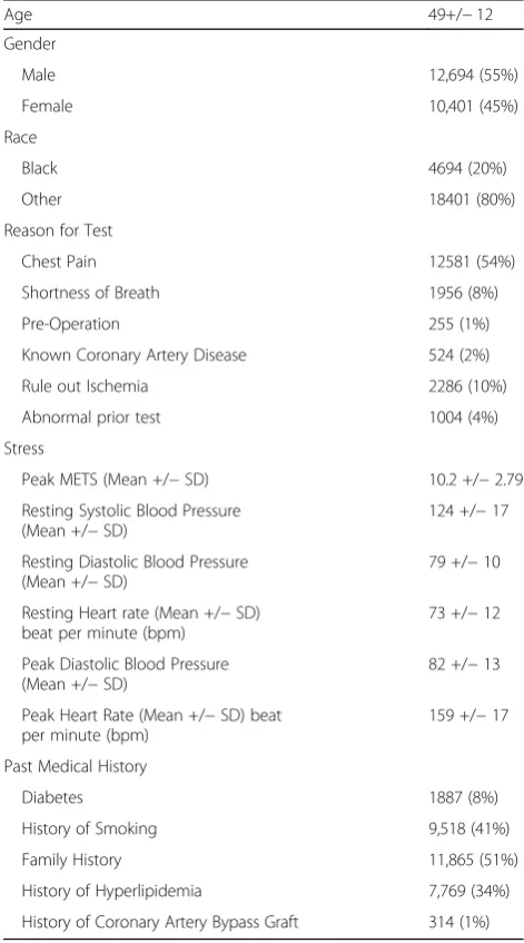
The dataset of this study has been collected from patients who underwent treadmill stress testing by physician refer-rals at Henry Ford Affiliated Hospitals in metropolitan Detroit, MI in the U.S. The data has been obtained from the electronic medical records, administrative databases, and the linked claim files and death registry of the hospital [52]. Study participants underwent routine clinical treadmill exercise stress testing using the standard Bruce protocol between January 1st, 1991 and May 28th, 2009. The total number of patients included in this study is (n= 23,095). The data set includes 43 attributes containing information on vital signs, diagnosis and clinical laboratory measure-ments. The baseline characteristics of the included cohort are shown in Table1. The dataset contains 23,095 individ-uals (12,694 males (55%) and 10,401 (45%) females) with ages that range between 17 and 96. Half of the patients have a family history of cardiovascular diseases. During the 10-years follow-up, around 35% of the patients experienced hypertension. Male hypertension patients represent around 55% of the total hypertension patients while female patients
Fig. 1The interpretability process of black box machine learning algorithms
Table 1Dataset Description (Cohort Characteristics)
Age 49+/−12
Gender
Male 12,694 (55%)
Female 10,401 (45%)
Race
Black 4694 (20%)
Other 18401 (80%)
Reason for Test
Chest Pain 12581 (54%)
Shortness of Breath 1956 (8%)
Pre-Operation 255 (1%)
Known Coronary Artery Disease 524 (2%)
Rule out Ischemia 2286 (10%)
Abnormal prior test 1004 (4%)
Stress
Peak METS (Mean +/−SD) 10.2 +/−2.79
Resting Systolic Blood Pressure (Mean +/−SD)
124 +/−17
Resting Diastolic Blood Pressure (Mean +/−SD)
79 +/−10
Resting Heart rate (Mean +/−SD) beat per minute (bpm)
73 +/−12
Peak Diastolic Blood Pressure (Mean +/−SD)
82 +/−13
Peak Heart Rate (Mean +/−SD) beat per minute (bpm)
159 +/−17
Past Medical History
Diabetes 1887 (8%)
History of Smoking 9,518 (41%)
Family History 11,865 (51%)
History of Hyperlipidemia 7,769 (34%)
represent around 44% of the total hypertension patients. For more details about the dataset, the process of develop-ing the prediction model and the FIT project, we refer the reader to [21,52].
In the following, we highlight the interpretability methods that are used in this study.
Global interpretability techniques
Table 2 summarizes the main features of the model-ag-nostic interpretability techniques used in this study. In the following, we list and explain each of them.
Feature Importance
It is a global interpretation method where the feature importance is defined as the increase in the model’s prediction error after we permuted the values of the features (breaks the relationship between the feature and the outcome) [53]. A feature is considered important if permuting its values increase the error (degrade the performance).
Partial Dependence Plot (PDP)
It is a global interpretation method where the plot shows the marginal effect of a single feature on the predicted risk of hypertension of a previously fit model [54]. The prediction function is fixed at a few values of the chosen features and averaged over the other features. Partial dependence plots are interpreted in the same way of a regression model which makes its interpretation easy. The main disadvantage of the partial dependence plot is the assumption that the feature of which the PDP is computed to be completely independent distributed from the other features that we average over.
Individual Conditional Expectation (ICE)
The partial dependence plot aims to visualize the average effect of a feature on the predicted risk of hypertension.
Partial dependence is a global method as it does not focus on specific instances but on an overall average. ICE plot can be seen as the disaggregated view of PDP by display-ing the estimated functional relationship for each instance in the dataset. The partial dependence plot can be seen as the average of the lines of an ICE plot [55]. In other words, ICE visualizes the dependence of the predicted risk of hypertension on particular features for each instance in the dataset. One main advantage of the ICE is that is easier to understand and more intuitive to interpret than the PDP. ICE suffers from the same disadvantage of PDP.
Feature Interaction
It is a global interpretation method where the interaction between two features represents the change in the predic-tion that occurs by varying the 13 features, after having accounted for the individual feature effects. It presents the effect that comes on top of the sum of the individual feature effects. One way to measure the interaction strength is to measure how much of the variation of the predicted outcome depends on the interaction of the features. This measure is known as H-statistic [56]. One of the main advantages of the feature interaction is that it considers the interaction between the features. The main disadvantage of the feature interaction is that it is compu-tationally expensive as it iterates over all the instances in the dataset.
Global Surrogate Models
It is a global interpretation method which aims to ap-proximate the predictions of a complex machine learning models (such as neural networks) using a simple interpretable machine learning models (such as linear regression) [57]. Global surrogate models are considered model-agnostic methods as they do not require any information about the internal workings and the hyper-parameters settings of the black-box
Table 2Main features of the model-agnostic interpretability techniques used in this study
Technique Global Local Advantages Disadvantages
Feature Importance ✓ •Highly compressed global interpretation •Consider interactions between features
Unclear whether it can be used on training dataset or testing dataset
Partial Dependence Plot ✓ Intuitive and clear interpretation Assumption of independence between features
Individual Conditional Expectation
✓ Intuitive and easy to understand Plot can become overcrowded to understand
Feature Interaction ✓ Detects all interactions been features Computationally expensive
Global Surrogate Models ✓ Easy to measure the goodness of your surrogate model using R-squared measure
Not clear what is the best cut-off for R-squared to trust the resulted surrogate model
Local Surrogate Model (LIME) ✓ •Short and comprehensible explanation. •Explains different types of data (tabular,
text and image)
•Instability of the explanation
•Very close points may have totally different explanations
Shapley Value Explanations ✓ Explanation is based on strong game theory theorem
Computationally very expensive
model. One way to obtain a surrogate model is as fol-lows. Train an interpretable model such as logistic re-gression or decision tree on the same dataset used to train the black-box model (or a dataset that has the same distribution) such that target for the interpret-able model is the predictions of the black-box model. The main advantage of the surrogate models is its flexibility, in addition, it is easy to assess how well it approximates the black-box model. However, it is still problematic how well the surrogate model should approximate the black-box model in order to be trusted.
Local interpretability techniques
Local Surrogate Models (LIME)
It is a local model agnostic interpretation method which focuses on explaining the prediction of a single predic-tion of any black-box machine learning model locally (within the neighborhood of the prediction instance to be explained) [58]. The idea of LIME is quite intuitive, it generates a new dataset that consists of perturbed sam-ples and then gets the associated predictions from the black box model. Next, LIME weight perturbed samples by how close they are from the point to be explained where the closer the point form the point to be ex-plained, the higher weight it takes. Then, LIME fits an
interpretable model (such as linear regression) on the weighted sampled instances. The learned model should be a good approximation of the machine learning model locally, but not globally.
Shapley Value Explanations
It is a local interpretation method from game theory [59]. This interpretation method assumes that each feature in the instance to be explained is a ‘player’ in a game and the prediction is the payout. The Shapley value aims to distribute the payout among the fea-tures in a fair way. The main idea of Shapley value is that for each feature f in the instance to be explained, evaluate the model using all possible coalitions (sets) of features with and without f. Such approach is ex-tremely computationally expensive as the number of the coalitions increases exponentially with the number of features. Strumbelj and Kononenko [57], presented an approximation algorithm for Shapley Values using Monte-Carlo sampling technique. This approximation algorithm has been used in this work as an example of local explainer and will be referred to as Shapley Values explainer.
The analysis of the global and local machine learning interpretability techniques has been conducted using
based ML packages (Version 3.3.1) (https://www.r-pro-ject.org/).
Results
In this section we present the results of applying vari-ous gloal and local interpretability techniques for our predictive model for the individuals at risk of devel-oping hypertension based on cardiorespiratory fitness data. In particular, we present the results of Five glo-bal interpretability techniques, namely, feature import-ance, partial dependence plot, individual conditional expectation, feature interaction and global surrogate models. In addition, we present the results of 2 local
explanation techniques, namely, LIME and Shapley value explanation.
Global interpretability techniques
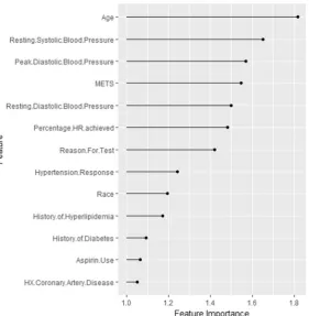
Feature Importance
Figure 2 shows the ranking of the importance of the selected input features in predicting the high risk of hypertension. The feature importance represents the factor by which the error is increased compared to the ori-ginal model error. As shown in the figure,Ageis the most important feature, followed byResting Systolic Blood Pres-sure. TheHistory of Coronary Artery Disease is the least significant feature.
Fig. 3Partial dependence plots for the highly ranked features for predicting hypertension
Fig. 4The interaction strength for each of the input features with all other features for predicting the high risk of hypertension
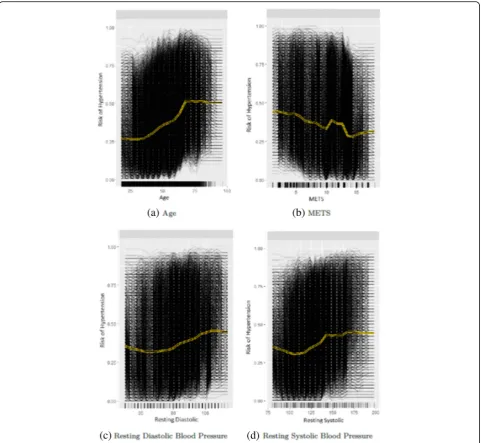
Partial Dependence Plot and Individual conditional expectation plot
The yellow line in Fig. 3 shows the partial dependence plot of the probability of high risk of hypertension for each of the highly ranked features for predicting hyper-tension: Age, METS,Resting Systolic Blood Pressure and Resting Diastolic Blood Pressure. The black lines in Fig.3 show the individual conditional expectation plot of the high risk of hypertension probability of the features. Each of the black lines represents the conditional ex-pectation for one patient. For theAgefeature, the partial
dependence plot shows that, on average, the probability of high risk of hypertension increases gradually from 0.25 to reach 0.5 at the age of 65 and then remain stable till the age of 100 (Fig. 3a). For the METS feature, the partial dependence plot shows that, on average, the in-crease inMETS is associated with a lower probability of high risk of hypertension (Fig. 3b). On average, the in-crease in theResting Diastolic Blood Pressureis associated with a gradual increase in the probability of high risk of hypertension (Fig.3c). For theResting Systolic Blood Pres-sure, the plot shows that the probability of high risk of
Fig. 6The terminal nodes of a surrogate tree of depth equals to 4 that approximates the behavior of the black box random forest model trained on the hypertension dataset
hypertension increases from 0.30 to 0.40 at METS around 140, then slightly fluctuating around 0.40 (Fig.3d).
Feature Interaction
Figure 4 shows the interaction strength for each of the input features with all other features for predicting the probability of high risk of hypertension. TheAgehas the highest interaction effect with all other features, followed by the Resting Systolic Blood Pressure. The History of Diabeteshas the least interaction with all other features. Overall the interaction effects between the features are considerably strong.
Global Surrogate Models
We fit a decision tree of depths equal to 3 and 4, using the original dataset, but with the prediction of the model
(Random Forest) used as an outcome for the decision tree model, instead of the real classes (high risk of hypertension and low risk of hypertension) from the ori-ginal dataset. Figures 5 and 6 show the terminal nodes of a surrogate decision tree of depth equals to 3 and 4 respectively. The counts in the nodes show the distribu-tion of the random forest model predicdistribu-tions in the nodes. The counts in the nodes in Fig. 5 show that the surrogate tree predicts a higher number of low risk of hypertension patients when theAgeis less than or equal to 50:2, Resting Diastolic Blood Pressure is less than or equal to 83 andMETSis less than or equal to 12:9. Also, the counts show that the surrogate tree of depth 3 pre-dicts a higher number of high risk of hypertension pa-tients when theAgeis greater than 50:2,Resting Systolic Blood Pressure is between 126 and 140. One way to
Fig. 7LIME explanation for Instance 1 as True Negative
measure how well the surrogate replicates the black box model is the R-squared measure. The surrogate tree of depth 3 has an R-squared (variance explained) around 0: 3 which means that the tree model of depth 3 approxi-mates the underlying Random Forest behavior very poorly. The counts of the nodes in Fig.6 show that the surrogate tree of depth 4 predicts a higher number of low risk of hypertension patients when the Age is less than or equal to 50.2,Resting Diastolic Blood Pressureis less than or equal to 83, METS is less than or equal to 12.9 and Hypertension Response is false. The counts in Fig. 6 also shows that the surrogate model predicts a higher number of high risk of hypertension patients when the Age greater than 50.2, Resting Systolic Blood Pressure is between 140 and 160. The R-squared of the surrogate model of depth 4 increases slightly to 0.4, however, when compared to the surrogate tree of depth
3, the model still does not approximate the black-box model (Random Forest) well.
Local interpretability techniques
The explanatory plot produced by the LIME explanation mechanism illustrates for each feature and class, in which the range of values of a representative data point would fall. If it does, this gets counted as support for this prediction and if it does not, it gets scored as contradict-ory. In addition, LIME produces what is so-called Explanation fitthat refers to the R-squared of the linear Ridge regression model which is fitted locally to explain the variance in the neighborhood of the examined instance. The explanatory plot produced by the Shapley Values explainer is close to the one generated by LIME in the sense that it shows the features’ names and fea-tures’contributions that are used in the explanation. A
Fig. 9LIME explanation for Instance 2 as True Positive
Fig. 10Shapley explanation for Instance 2 as True Positive
feature with a positive contribution value means that the feature contributes toward increasing the prediction of the model and a feature with a negative value means that the feature contributing toward decreasing the model’s output. The sum of all features’contributions is the dif-ference between the black-box model output and the model’s output when no information is given about fea-tures’ values. Therefore, we can measure the change in the model’s output and hence identify the features that contribute to this change and the amount of each fea-ture-value’s influence.
Since LIME and Shapley Values explainers are instance based explainers, in the following we evaluate both explainers based on 20 randomly selected instances from the testing dataset. In the following, we present the explanation of 20 instances in detail. We present 2 instances that have been correctly predicted by the black-box prediction model, one instance from theTrue Positive(correctly predicted as high risk of hypertension)
group and another instance for the True Negative (cor-rectly predicted as low risk of hypertension) group. In general, the generated explanations for the correctly pre-dicted instances are commonly very intuitive and clear. They mostly follow common standard patterns. Thus, we chose to more focus on the incorrectly predicted instances as understanding the rationale and explanations for such incorrect predictions of the model increases the trust of the clinicians on the model behavior and perform-ance. Thus, we present instances that comprehensively cover the False Positive and False Negative groups with consideration of the most important prediction factor, the patient’s age.
Instance 1 (True negative)
The description of this instance is as follows: Age = 36, METS = 13, Resting Systolic Blood Pressure = 80, Peak Dia-stolic Blood Pressure = 70, Resting DiaDia-stolic Blood Pres-sure = 60, HX Coronary Artery Disease = false, Reason for test = chest pain, HX Diabetes = false, Percentage HR achieved = 0.98, Race = white, Hx Hyperlipidemia = false, Aspirin Use = false, Hypertension Response = false.Figure7 shows LIME explanation of the prediction of instance 1 as low risk of hypertension with a strong probability of 0:98. The explanation is created based on five features Age, METS, Race, Reason for test and Aspirin Use.
Figure8shows Shapley explanation of instance 1 based on five featuresAge, METS,Percentage HR achieved, Rest-ing Diastolic Blood Pressure and Resting Systolic Blood Pressure. TheAge,METSare the most important features that contributed to the prediction of low risk of hyperten-sion for both LIME and Shapley. The explanations show that young patients under the age of 40s are at lower risk of developing hypertension compared to people above 40s
Fig. 11Histogram of false positive instances
which matches the partial dependence plot created in Fig. 3a and comes inline with the medical study by Rockwood et al. [60]. The explanations also show that those people whose METS are greater than 12:9 are at low risk of devel-oping hypertension which matches the medical study by Juraschek et al. [61]. LIME explanation also shows that white people are at lower risk of developing hypertension compared to black people which is supported by the study conducted by Ergul et al. [62].
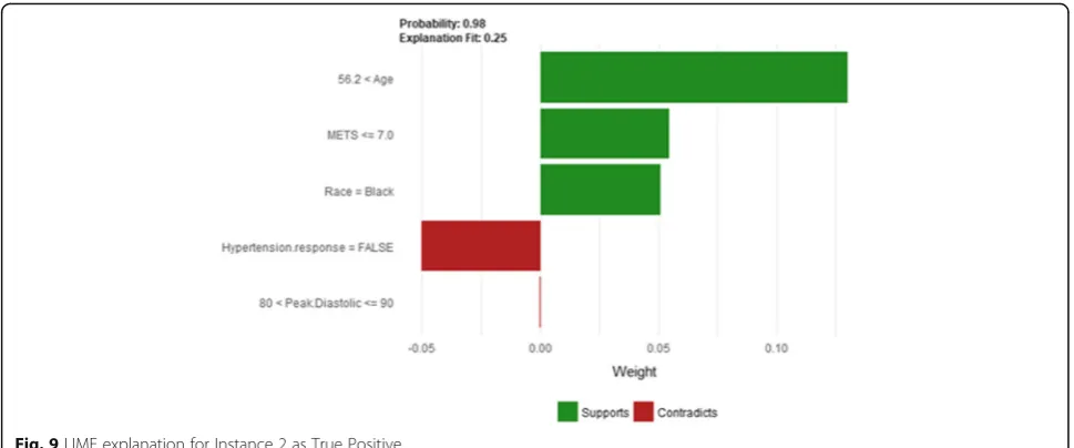
Instance 2 (True Positive)
The description of this instance is as follows:Age = 64.8, METS = 7, Resting Systolic Blood Pressure = 110, Peak
Diastolic Blood Pressure = 90, Resting Diastolic Blood Pressure = 70, HX Coronary Artery Disease = True, Reason for test = HX Coronary Artery Disease, HX Dia-betes = false, Percentage HR achieved = 0.79, Race = black, Hx Hyperlipidemia = false, Aspirin Use = false, Hyperten-sion Response = False.
Figure9shows the LIME explanation of the prediction of the black-box model for instance 2 as high risk of hypertension (assigning a strong probability of 0.98 for high risk of hypertension). The explanation is created based on five features Age, METS, Race, Hypertension Response, and Peak Diastolic Blood Pressure. The three features Age, METS, and Race positively support the
Fig. 13Shapley Values explanation of Instance 3 as False Positive Prediction of High Risk - Group 1 - Close to Maximum Age
Fig. 14LIME explanation of Instance 4 as False Positive Prediction of High Risk - Group 1 - Close to Minimum Age
explanation as a high risk of hypertension. Having nega-tive Hypertension Response test neganega-tively contributed to the explanation of the high risk of hypertension which is inline with the medical study by Zanettini et al. [63].
Figure 10 shows the Shapley Values explanation of
instance 2 as high risk of hypertension. The explanation is based on five featuresRace, HX Coronary Artery Dis-ease, Peak Diastolic Blood Pressure, Reason for test and Age that all contribute toward decreasing of the prob-ability of high risk of hypertension.
In the following, we are going to have a deep look at the misclassified instances by the Random Forest model and see the explanation using LIME. To ensure diversity, we selected nine instances from each of the False Positive instances (incorrectly classified as
high risk of hypertension) and False Negative
instances (incorrectly classified as low risk of
hypertension) based on the patient’s age as it has been identified to be the most important feature based on the feature importance plot and the partial dependence plot.
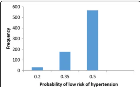
We start studying false positive instances. Figure 11 shows the frequency distribution of the false positive instances based on the probability of low risk of hyper-tension. The probability of low risk of hypertension has been split into three groups (bins). Group 1 represents instances with the probability of low risk of hypertension between [0–0.2]. Group 2 and Group 3 represent in-stances with the probability of low risk of hypertension that belongs to]0.2–0.35] and]0.35–0.5[, respectively. The frequency of the instances in group three is the highest (the black-box model predicts a patient as low risk of hypertension if the low-risk probability is greater than or equal to 0.5). In the following, we present
Fig. 15Shapley explanation of Instance 4 as False Positive Prediction of High Risk - Group 1 - Close to Minimum Age
sample instances from each of the three groups selected based on the patient’s age.
In the following, we present sample instances ofFalse Positivepredictions fromGroup 1. The instances are se-lected based on the patient’s age: one instance is close to the maximum age, one instance is close to the minimum age and one instance close to average age.
Instance 3 (False Positive Prediction of High Risk Group 1 -Close to Maximum Age)
The description of this instance is as follows: Age = 75.39, METS = 6.4, Resting Systolic Blood Pressure = 150, Peak Diastolic Blood Pressure = 90, Resting Diastolic Blood Pressure = 94, HX Coronary Artery Disease = false, Reason for test = HX Coronary Artery Disease, HX
Diabetes = false, Percentage HR achieved = 1.04, Race = white, Hx Hyperlipidemia = true, Aspirin Use = true, Hypertension Response = true.
Figure12 shows LIME explanation of instance 3 based onAge,Resting Systolic Blood Pressure,METS,Percentage HR achieved, andPeak Diastolic. All the features used in the explanation positively contributed to the prediction of the high risk of hypertension with a probability equals to 0.68. Figure 13shows the Shapley Values explanation of instance 3 based onPercentage HR achieved,Aspirin Use, METS,Age, andReason for test. The most contributed fea-ture toward increasing the probability high risk of hyper-tension isPercentage HR achievedwhileReason for testis the most contributed feature toward decreasing the prob-ability of the high risk of hypertension.
Fig. 17Shapley explanation of Instance 5 as False Positive Prediction of High Risk - Group 1 - Close to Average Age
Fig. 18LIME explanation of instance 6 as False Positive Prediction of high Risk - Group 2 - Close to Maximum Age
Instance 4 (False Positive Prediction of High Risk Group 1 -Close to Minimum Age)
The description of this instance is as follows:Age = 53.77, METS = 10.1, Resting Systolic Blood Pressure = 166, Peak Diastolic Blood Pressure = 90, Resting Diastolic Blood Pres-sure = 90, HX Coronary Artery Disease = false, Reason for test = Chest Pain, HX Diabetes = false, Percentage HR achieved = 0.93, Race = white, Hx Hyperlipidemia = true, Aspirin Use = false, Hypertension Response = true.
Figure 14 shows LIME explanation of instance 4 as high risk of hypertension with a probability of 0.7. The explanation shows that Resting Diastolic Blood Pressure, Resting Systolic Blood Pressure and Hypertension Response are the most important features that positively strongly contributed to the prediction of high risk of hypertension while being white negatively contributed to the prediction of high risk of hypertension. Figure 15 shows Shapley Values explanation of instance 4 as high
risk of hypertension based onReason for test,Hx Hyper-lipidemia, Resting Diastolic Blood Pressure, Resting Sys-tolic Blood Pressure and METS. The most contributed feature toward increasing the probability high risk of hypertension isReason for test while METS is the most contributed feature toward decreasing the probability of the high risk of hypertension.
Instance 5 (False Positive Prediction of High Risk Group 1 -Close to Average Age)
The description of this instance is as follows:Age = 67.9, METS = 6, Resting Systolic Blood Pressure = 114, Peak Diastolic Blood Pressure = 88, Resting Diastolic Blood Pressure = 78, HX Coronary Artery Disease = true, Reason for test = HX Coronary Artery Disease, HX Dia-betes = false, Percentage HR achieved = 0.94, Race = white, Hx Hyperlipidemia = true, Aspirin Use = false, Hypertension Response = false
Fig. 19Shapley explanation of instance 6 as False Positive Prediction of high Risk - Group 2 - Close to Maximum Age
TheAgeandMETSare the most important features for LIME that positively contributed to the prediction of high risk of hypertension while being white and has negative Hypertension Response test negatively contributed to the prediction of high risk of hypertension as shown in Fig.16. LIME explains instance 5 as high risk of hypertension with a probability of 0.68. Figure17shows Shapley Values ex-planation of instance 5 based on Resting Systolic Blood Pressure, HX Coronary Artery Disease, METS,Reason for testandAge. All the features exceptResting Systolic Blood Pressure contributed toward decreasing the probability of the high risk of hypertension.
In the following, we present sample instances ofFalse Positive predictions from Group 2. The instances are selected based on the patient’s age: one instance is close
to the maximum age, one instance is close to the mini-mum age and one instance close to average age.
Instance 6 (False Positive Prediction of high Risk Group 2 -Close to Maximum Age)
The description of this instance is as follows: Age = 82.23, METS = 7, Resting Systolic Blood Pressure = 164, Peak Diastolic Blood Pressure = 80, Resting Diastolic Blood Pressure = 80, HX Coronary Artery Disease = false, Reason for test = Rule out Ischemia, HX Diabetes = false, Percentage HR achieved = 1.09, Race = white, Hx Hyper-lipidemia = false, Aspirin Use = false, Hypertension Re-sponse = false
Figure18shows the explanation of instance 6 as high risk of hypertension with a weak probability of 0.64. The
Fig. 21Shapely explanation of Instance 7 as False Positive Prediction of High Risk - Group 2 - Close to Minimum Age
Fig. 22LIME explanation of Instance 8 as False Positive Prediction of High Risk - Group 2 - Close to Average Age
explanation is based onAge,Resting Systolic Blood Pres-sure, METS, Hypertension Response, and Aspirin Use. Age,Resting Systolic Blood Pressure and METSare posi-tively contributed to the probability of high risk of hypertension while negative Hypertension Response test and not using aspirin are negatively contributed to the prediction of high risk of hypertension. Figure 19shows the Shapley Values explanation of instance 6 as high risk of hypertension based onPeak Diastolic Blood Pressure, Reason for test, METS, Resting Systolic Blood Pressure, and Age. All the features except Peak Diastolic Blood Pressure contributed toward decreasing the probability of the high risk of hypertension
Instance 7 (False Positive Prediction of High Risk Group 2 -Close to Minimum Age)
The description of this instance is as follows: Age = 42.81, METS = 10, Resting Systolic Blood Pressure = 140, Peak Diastolic Blood Pressure = 98, Resting Diastolic
Blood Pressure = 86, HX Coronary Artery Disease = false, Reason for test = shortness of breath, HX Diabetes = false, Percentage HR achieved = 0.92, Race = white, Hx Hyper-lipidemia = true, Aspirin Use = false, Hypertension Re-sponse = true.
Figure 20shows LIME explanation of instance 7 as
high risk of hypertension with a weak probability of
0.6. The explanation is based on Resting Diastolic
Blood Pressure, Resting Systolic Blood Pressure, Hyper-tension Response, Age and METS. All the features used in the explanation except Age are positively con-tributed to the probability of high risk of hyperten-sion. Figure 21 shows Shapley Values explanation of instance 7 as high risk of hypertension based on Age, Resting Diastolic Blood Pressure, Resting Systolic Blood Pressure, Peak Diastolic Blood Pressure, and Hyperten-sion Response. All the features except Age contributed toward decreasing the probability of the high risk of hypertension.
Fig. 23Shapley explanation of Instance 8 as False Positive Prediction of High Risk - Group 2 - Close to Average Age
Instance 8 (False Positive Prediction of High Risk Group 2 -Close to Average Age)
The description of this instance is as follows:Age= 59.9, METS= 10.1, Resting Systolic Blood Pressure= 124, Peak Diastolic Blood Pressure= 90, Resting Diastolic Blood Pressure= 80, HX Coronary Artery Disease= false, Rea-son for test= chest pain, HX Diabetes= true, Percentage HR achieved= 0.675,Race= white, Hx Hyperlipidemia= false,Aspirin Use= false,Hypertension Response= false
Figure22shows LIME explanation of instance 8 based onAge,Hypertension Response,Race,Reason for testand Peak Diastolic Blood Pressure. Age and Peak Diastolic Blood Pressure contributed positively to the prediction of high risk of hypertension with a probability of 0:62, while Hypertension Response, Race, and Reason for test contributed negatively to the prediction of high risk of
hypertension. Figure 23 shows Shapley Values
explanation for instance 8 based on Resting Systolic Blood Pressure, Percentage HR achieved, Resting Dia-stolic Blood Pressure, Reason for test, and HX Diabetes. All the features except HX Diabetescontributed toward
increasing the probability of the high risk of
hypertension.
In the following, we present sample instances ofFalse Positive predictions from Group 3. The instances are selected based on the patient’s age: one instance is close to the maximum age, one instance is close to the mini-mum age and one instance close to average age.
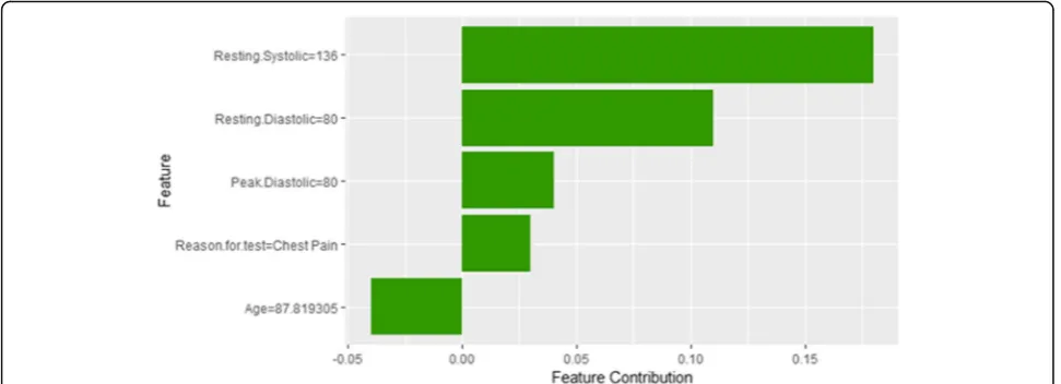
Instance 9 (False Positive Prediction of High Risk Group 3 -Close to Maximum Age)
The description of this instance is as follows: Age = 87.82, METS = 7, Resting Systolic Blood Pressure = 136, Peak Diastolic Blood Pressure = 80, Resting Diastolic
Fig. 25Shapley explanation of Instance 9 as False Positive Prediction of High Risk - Group 3 - Close to Maximum Age
Fig. 26LIME explanation of Instance 10 as False Positive Prediction of High Risk - Group 3 - close to Minimum Age
Blood Pressure = 80, HX Coronary Artery Disease = 0, Reason for test = chest pain, HX Diabetes = 0, Percentage HR achieved = 1.098, Race = white, Hx Hyperlipidemia = true, Aspirin Use = false, Hypertension Response = false.
Figure24shows LIME explanation of instance 9 based on Age, Resting Systolic Blood Pressure, METS, Reason for testandAspirin Use.Age,Resting Systolic Blood Pres-sureandMETSare the most contributed features for the prediction of the high risk of hypertension with a weak probability of 0.6. Figure 25 shows Shapley Values ex-planation of instance 9 based on Resting Systolic Blood Pressure, Peak Diastolic Blood Pressure, Reason for test and Age. All the features except Agecontributed toward increasing the probability of the high risk of hypertension.
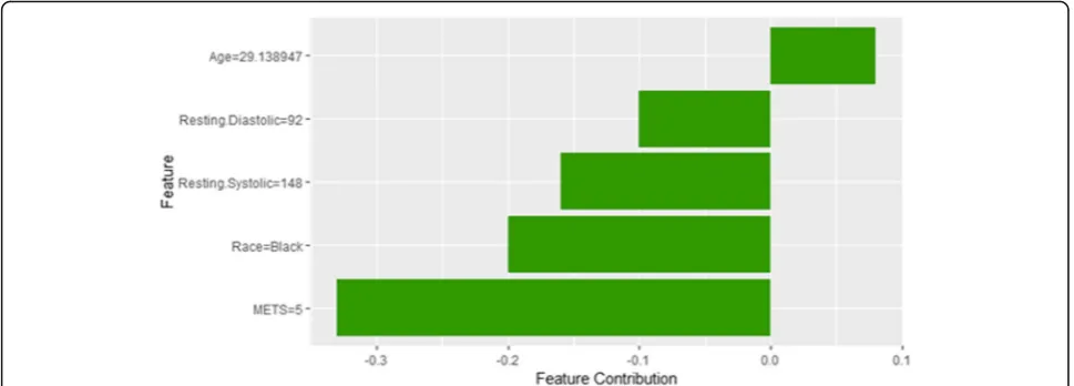
Instance 10 (False Positive Prediction of High Risk - Group 3 - close to Minimum Age)
The description of this instance is as follows: Age = 29.13, METS = 5, Resting Systolic Blood Pressure = 148,
Peak Diastolic Blood Pressure = 60, Resting Diastolic Blood Pressure = 92, HX Coronary Artery Disease = 0, Reason for test = Chest Pain, HX Diabetes = 0, Percentage HR achieved = 0.79, Race = black, Hx Hyperlipidemia = false, Aspirin Use = false, Hypertension Response = false.
Instance 10 is incorrectly predicted by the black box model as a high risk of hypertension with a weak prob-ability equals to 0.52 using LIME explainer as shown in Fig. 26. It is clear from the explanation that the young Age of the patient strongly contributed against the pre-diction of the high risk of hypertension while Resting Diastolic Blood Pressure, Resting Systolic Blood Pressure and METS contributed positively to the prediction of the high risk of hypertension. The explanation of in-stance 10 using Shapley Values is shown in Fig.27using features Age, Resting Diastolic Blood Pressure, Resting Systolic Blood Pressure,RaceandMETS. The featureAge is the only features contributed toward increasing the probability of high risk of hypertension.
Fig. 27Shapley explanation of Instance 10 as False Positive Prediction of High Risk - Group 3 - close to Minimum Age
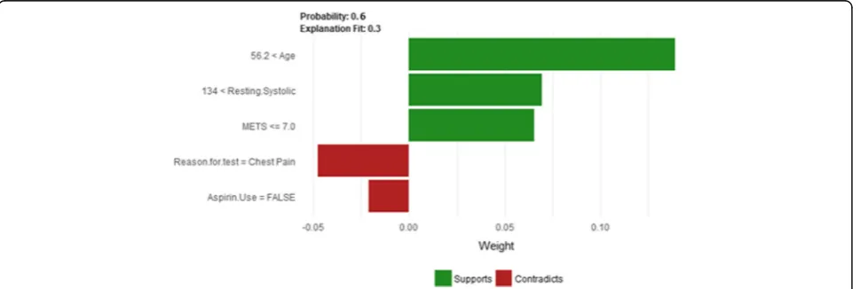
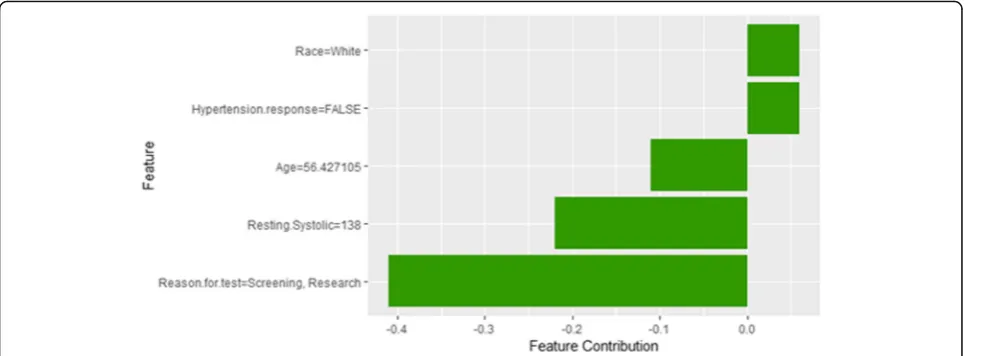
Instance 11 (False Positive Prediction of High Risk - Group 3 - Close to Average Age)
The description of this instance is as follows:Age = 56.4, METS = 7, Resting Systolic Blood Pressure = 138, Peak Diastolic Blood Pressure = 60, Resting Diastolic Blood Pressure = 82, HX Coronary Artery Disease = false, Rea-son for test = Screening, HX Diabetes = false, Percentage HR achieved = 0.87, Race = white, Hx Hyperlipidemia = false, Aspirin Use = false, Hypertension Response = false.
Figure28shows LIME explanation of instance 11 as a high risk of hypertension with a probability of 0.51. Fea-tures Age,Resting Systolic Blood Pressureand METS are the main features that contributed to the prediction of the high risk of hypertension. Shapley Values explan-ation for instance 11 is shown in Fig.29, based on Race, Hypertension Response, Age, Resting Systolic Blood Pres-sure, and Reason for test. The two features Race and Hypertension Response are the only features contributed toward the increasing probability of high risk of hyper-tension. The explanations of these False Positive exam-ples show that the Age is the most influencing feature
towards the explanation of the high risk of hypertension based on LIME. We noticed that instances in Group 3 have the lowest average age of 56, while instances in Group 1 has the highest average age of 68 amongst the three groups which clearly indicates that the probability of low risk of hypertension decreases with the increase in the patient’s age.
In the following, we are going to have a deep look at examples for instances that haveFalse Negative predica-tions (Incorrectly classified as low risk of hypertension). Figure 30 shows the frequency distribution of the false negative instances based on the probability of high risk of hypertension. The probability of high risk of hyper-tension has been split into another three groups.Group
4 represents instances with the probability of high risk of hypertension between [0–0.2].Group 5and Group 6 represent instances with a probability of high risk of hypertension belongs to]0.2–0.35] and]0.35–0.48[, respectively (0.48 is the highest probability in the False Negative instances). In particular, we present sample instances of False Negative predictions from Group 4. The instances are selected based on the patient’s age: one instance is close to the maximum age, one instance is close to the minimum age and one instance close to average age.
Instance 12 (False Negative Prediction of Low Risk - Group 4 - Close to Maximum Age)
The description of this instance is as follows:Age = 63.8, METS = 13, Resting Systolic Blood Pressure = 112, Peak Diastolic Blood Pressure = 80, Resting Diastolic Blood Pressure = 72, HX Coronary Artery Disease = false, Reason for test = Rule out Ischemia, HX Diabetes = false, Percentage HR achieved = 0.95, Race = white, Hx
Fig. 29Shapley explanation of Instance 11 as False Positive Prediction of High Risk - Group 3 - Close to Average Age
Fig. 30Histogram of false negative instances
Hyperlipidemia = false, Aspirin Use = false, Hypertension Response = false.
Figure31shows the explanation of instance 12 as low risk of hypertension with a strong probability of 0.8. The explanation is based on Age, METS, Race, Hypertension ResponseandReason for test.Ageis the most influencing feature that negatively contributed to the prediction of low risk of hypertension while METS, Race and Hyper-tension Response contributed positively to the prediction of low risk of hypertension. Figure 32 shows Shapley
values explanation for instance 12 based on METS,
Resting Systolic Blood Pressure, Hypertension Response, Reason for test, and Age. Similar to LIME explanation, features METS, and Hypertension Response contributed toward the probability of low risk of hypertension.
Instance 13 (False Negative Prediction of Low Risk - Group 4 - Close to Minimum Age)
The description of this instance is as follows:Age = 18.8, METS = 15, Resting Systolic Blood Pressure = 120, Peak Diastolic Blood Pressure = 90, Resting Diastolic Blood Pressure = 80, HX Coronary Artery Disease = false, Rea-son for test = Chest Pain,HX Diabetes = 0, Percentage HR achieved = 0.85, Race = black, Hx Hyperlipidemia = false, Aspirin Use = false, Hypertension Response = false.
Figure 33 shows the explanation of instance 13 based onAge,METS,Hypertension Response,Reason for testand Percentage HR achieved. All the features used in the ex-planation except Percentage HR achieved contributed positively to the prediction of low risk of hypertension (probability = 0.82). Figure 34 shows Shapley Values
Fig. 31LIME explanation of Instance 12 as False Negative Prediction of Low risk - Group 4 - Close to Maximum Age
explanation for instance 13 based onAge,Reasonfortest, Resting Diastolic Blood Pressure, Hypertension Response, METS. All the features in the explanation contributed to-ward the probability of low risk of hypertension
Instance 14 (False Negative Prediction of Low risk - Group 4 - Close to Average Age)
The description of this instance is as follows: Age = 48.26, METS = 12, Resting Systolic Blood Pressure = 110, Peak Diastolic Blood Pressure = 70, Resting Diastolic Blood Pressure = 70, HX Coronary Artery Disease = false, Reason for test = Chest Pain, HX Diabetes = false, Percentage HR achieved = 0.85, Race = white, Hx Hyper-lipidemia = false, Aspirin Use = false, Hypertension Re-sponse = false.
Figure 35 shows LIME explanation of instance 14
based on Hypertension Response, Age, Resting Systolic Blood Pressure, Reason for test and METS. All the
features used in the explanation except METS are posi-tively contributed to the prediction of low risk of hyper-tension (probability = 0.96). Figure 36 shows Shapley Values explanation for instance 14 based on the features ofResting Systolic Blood Pressure,Age,METS,Hx Hyper-lipidemia, and Resting Diastolic Blood Pressure. All the features contributed toward increasing the probability of low risk of hypertension.
In the following, we present sample instances ofFalse Negativepredictions fromGroup 5. The instances are se-lected based on the patient’s age: one instance is close to the maximum age, one instance is close to the minimum age and one instance close to average age.
Instance 15 (False Negative Prediction of Low Risk - Group 5 - Close to Maximum Age)
The description of this instance is as follows:Age = 79.6, METS = 7, Resting Systolic Blood Pressure = 120, Peak
Fig. 33LIME explanation of Instance 13 as False Negative Prediction of Low Risk - Group 4 - Close to Minimum Age
Fig. 34Shapley explanation of Instance 13 as False Negative Prediction of Low Risk - Group 4 - Close to Minimum Age
Diastolic Blood Pressure = 70, Resting Diastolic Blood Pressure = 64, HX Coronary Artery Disease = 0, Reason for test = Chest Pain,HX Diabetes = false, Percentage HR achieved = 0.96, Race = white, Hx Hyperlipidemia = true, Aspirin Use = false, Hypertension Response = true.
Figure37 shows the explanation of instance 15 based on Age, METS, Hypertension Response, Reason for test and Peak Diastolic Blood Pressure. All the features used in the explanation exceptAgeandMETSare contributed positively to the prediction of low risk of hypertension with probability equals to 0.7. Shapley Values explan-ation for instance 15, shown in Fig. 38, is based on the same five features used by LIME except forHypertension Response is replaced by Resting Systolic Blood Pressure. Peak Diastolic Blood PressureandAgeare the most con-tributing features toward increasing and decreasing the probability of low risk of hypertension respectively.
Instance 16 (False Negative Prediction of Low Risk - Group 5 - Close to Minimum Age)
The description of this instance is as follows: Age = 22.78, METS = 12.9, Resting Systolic Blood Pressure = 112, Peak Diastolic Blood Pressure = 64, Resting Diastolic Blood Pressure = 68, HX Coronary Artery Disease = false, Reason for test = Dizzy, HX Diabetes = false, Percentage HR achieved = 1.01, Race = white, Hx Hyperlipidemia = true, Aspirin Use = false, Hypertension Response = false.
Figure39shows LIME explanation of instance 16 based on Age, Race, Hypertension Response, Resting Systolic Blood Pressure and METS. All the features used in the explanation except METS contributed positively to the prediction of low risk of hypertension with a strong prob-ability of 0.86. Figure40shows Shapley Values explanation of instance 16 based on features Age, Percentage HR achieved, Peak Diastolic Blood Pressure, Resting Diastolic
Fig. 35LIME explanation of Instance 14 as False Negative Prediction of Low risk - Group 4 - Close to Average Age
Blood Pressure, and Hypertension Response. All the fea-tures used in the explanation contributed toward increas-ing the probability of low risk of hypertension.
Instance 17 (False Negative Prediction of Low Risk - Group 5 - Close to Average Age)
The description of this instance is as follows: Age = 48.78, METS = 10.1, Resting Systolic Blood Pressure = 110, Peak Diastolic Blood Pressure = 70, Resting Diastolic Blood Pres-sure = 70, HX Coronary Artery Disease = false, Reason for test = Rule out Ischemia,HX Diabetes = 0, Percentage HR achieved = 0.92, Race = black, Hx Hyperlipidemia = false, Aspirin Use = false, Hypertension Response = false.
Figure41shows the explanation of instance 17 based on HX Diabetes, Hypertension, Response, Race, Resting Sys-tolic Blood Pressure and METS. All the features used in the explanation except being black are contributed to the
prediction of low risk of hypertension with a probability of 0.72. Figure 42 shows Shapley Values explanation of in-stance 17 which is based on Hx Hyperlipidemia, Resting Diastolic Blood Pressure, Resting Systolic Blood Pressure, Age and Peak Diastolic Blood Pressure. All the features contributed toward increasing the probability of low risk of hypertension.
In the following, we present sample instances ofFalse Negative predictions from Group 6. The instances are selected based on the patient’s age: one instance is close to the maximum age, one instance is close to the mini-mum age and one instance close to average age.
Instance 18 (False Negative Prediction of Low Risk - Group 6 - Close to Maximum Age)
The description of this instance is as follows:Age= 78.2, METS= 7, Resting Systolic Blood Pressure= 110, Peak
Fig. 37LIME explanation of Instance 15 as False Negative Prediction of Low Risk - Group 5 - Close to Maximum Age
Fig. 38Shapley explanation of Instance 15 as False Negative Prediction of Low Risk - Group 5 - Close to Maximum Age
Diastolic Blood Pressure= 84, Resting Diastolic Blood Pressure= 72, HX Coronary Artery Disease= false, Rea-son for test= chest pain, HX Diabetes= false, Percentage HR achieved= 0.96, Race= white, Hx Hyperlipidemia= false,Aspirin Use= false,Hypertension Response= false.
Figure 43 shows LIME explanation of instance 18
based on Age, METS, Race, Reason for test, and Peak Diastolic Blood Pressure. Race and Reason for test contributed positively to the prediction of low risk of hypertension with a weak probability of 0.6. Figure 44 shows Shapley Values explanation of instance 18
which is based on Resting Systolic Blood Pressure,
Resting Diastolic Blood Pressure, Reason for test, and Peak Diastolic Blood Pressure, Age. All the features
except Age contributed toward increasing the
prob-ability of low risk of hypertension.
Instance 19 (False Negative Prediction of Low Risk - Group 6 - Close to Minimum Age)
The description of this instance is as follows: Age = 27.8, METS = 10.1, Resting Systolic Blood Pressure = 112, Peak Diastolic Blood Pressure = 110, Resting Diastolic Blood Pres-sure = 80, HX Coronary Artery Disease = false, Reason for test = shortness of breath, HX Diabetes = false, Percentage HR achieved = 0.86, Race = white, Hx Hyperlipidemia = false, Aspirin Use = false, Hypertension Response = false.
Figure45 shows the explanation of instance 19 based on Age, Hypertension Response, Race, Resting Diastolic Blood Pressure and METS and. All the features used in the explanation contributed positively to the prediction of low risk of hypertension with a probability of 0.7. Figure46 shows the Shapley Values explanation of instance 19 which is based onAge, Hx Hyperlipidemia, Hypertension
Fig. 39LIME explanation of Instance 16 as False Negative Prediction of Low Risk - Group 5 - Close to Minimum Age
Response, Resting Systolic Blood Pressure, and METS. All the features exceptMETS contributed toward increasing the probability of low risk of hypertension.
Instance 20 (False Negative Prediction of Low Risk - Group 6 - Close to Average Age)
The description of this instance is as follows: Age = 48.5, METS = 5, Resting Systolic Blood Pressure = 110, Peak Dia-stolic Blood Pressure = 88, Resting DiaDia-stolic Blood Pres-sure = 78, HX Coronary Artery Disease = false, Reason for test = shortness of breath, HX Diabetes = false, Percentage HR achieved = 0.9, Race = white, Hx Hyperlipidemia = false, Aspirin Use = false, Hypertension Response = false.
Figure 47 shows LIME explanation of instance 20
based on METS, Race, Hypertension Response, Resting Diastolic Blood Pressureand Peak Diastolic Blood Pres-sure. All the features used in the explanation except
METS and Peak Diastolic Blood Pressure contributed to the prediction of low risk of hypertension with a weak probability of 0.54. Figure 48 shows the Shapley Values explanation of instance 20 based on Hx Hyperlipidemia, Peak Diastolic Blood Pressure, METS, Age, and Reason for test. All the features used in the explanation except Hx Hyperlipidemia contributed toward decreasing the probability of low risk of hypertension.
Discussion
In general, the global interpretability techniques have the advantage that it can generalize over the entire population while local interpretability techniques give explanations at the level of instances. Both methods may be equally valid depending on the application need. For example, a healthcare application such as predicting the progression of risk of hypertension may require global
Fig. 41LIME explanation of Instance 17 as False Negative Prediction of High Risk - Group 5 - Close to average age
Fig. 42Shapley explanation of Instance 17 as False Negative Prediction of High Risk - Group 5 - Close to average age
understanding for the main risk factors for developing hypertension. In this case, local explainers may not be suitable. One way to meet the application goal is to use the global explanation methods. Another way to meet the application requirements using local explainers is to get local explanations and then aggregate them to gener-ate global level explanations. Such technique is compu-tationally expensive.
One of the main advantages of LIME is that its explan-ation is based on the local regression model, which allow physicians to make statements about changes in expla-nations for changes in the features of the patient to be explained, for example, “what would the probability of hypertension if the patients after five years?”. One of the main limitations of LIME is the instability of the expla-nations. Patients with very close characteristics may have
very different explanations. Even for a single patient, if you get the explanation twice, you may get two different explanations. Another limitation is the perturbed data points that act as the training data for the interpretable model are sampled from Gaussian distribution that ignores the correlation between features. This may lead to poor selection of data points that result in poor explanation. LIME assumes a strong assumption that the local model fitted on the perturbed data is linear, how-ever, there is no clear theory about the validity of the assumption.
One of the main advantages that distinguish Shapley value explanation from LIME is that the difference between the average prediction and the prediction of the instance to be explained is fairly distributed among the feature values of the instance to be explained. In other
Fig. 43LIME explanation of Instance 18 as False Negative Prediction of Low Risk - Group 3 - Close to Maximum Age
words, Shapley, value explanation. On the other side, Shapley value explanation is computationally expensive. Another disadvantage is that we need to access the training examples used in training the model to be explained unlike LIME.
Many methods have been proposed to make complex machine learning model interpretable, however, these methods have been evaluated individually on small data-sets [60]. To the best of our knowledge, this is the first study that applies and demonstrates the utility of various model-agnostic explanation techniques of machine learn-ing models analyzlearn-ing the outcomes of prediction model for the individuals at risk of developing hypertension based on cardiorespiratory fitness data. This study is de-signed to take advantage of the unique and rich clinical re-search dataset consisting of 23,095 patients to explain the predictions of the best performing machine learning
model for predicting individuals at risk of developing hypertension in an understandable manner for clinicians. The results show that different interpretability tech-niques can shed light on different insights on the model behavior where global interpretations can en-able clinicians to understand the entire conditional distribution modeled by the trained response function. In contrast, local interpretations promote the under-standing of small parts of the conditional distribution for specific instances. In practice, both methods can be equally valid depending on the application need. Both methods are effective methods for assisting cli-nicians on the medical decision process, however, the clinicians will always remain to hold the final say on accepting or rejecting the outcome of the machine learning models and their explanations based on their domain expertise.
Fig. 45LIME explanation of Instance 19 as False Negative Prediction of Low Risk - Group 3 - Close to Minimum Age
Fig. 46Shapley explanation of Instance 19 as False Negative Prediction of Low Risk - Group 3 - Close to Minimum Age
Threats to validity
Extenral validity
A main limitation of this study is that the predictors of the models, the predictions of the models fot the new instances and the explanations of the interpretability techniques are all based on the charachteritsics and used predictors of the cohort of this study.
Construct validity
This study has been mainly focusing on two local inter-pretability techniques, namely, LIME and Shapley Value Explanations. The inclusion of additional local interpret-ability techniques may lead to different explanations and additional insights.
Conclusion Validity
Due to the nature of this study and the unlimited availabil-ity of similar comparable cohorts. Generalizing the findings and explanations of this study would require the inclusion of multiple datasets representing multiple cohorts.
Conclusion
Explaining the predictions of black-box machine learn-ing models have become a crucial issue which is gainlearn-ing increasing momentum. In particular, achieving optimal performance of the machine learning models have not become the only focus of data scientists, instead, there is growing attention on the need for explaining the predic-tions of black-box models on both global and local levels. Several explanations that have been produced by
Fig. 47LIME explanation of Instance 20 as False Negative Prediction of Low Risk - Group 3 - Close to Average Age
various methods in this study reflect the significant role of these techniques in assisting the clinical staff in the decision-making process. For example, the LIME tech-nique can allow physicians to make statements about changes in explanations for changes in the features of the patient to be explained. However, the LIME tech-nique suffers from the instability of the explanations. Meanwhile, the Shapley value explanation technique has shown the ability to demonstrate that the difference between the average prediction and the prediction of the instance to be explained is fairly distributed among the feature values of the instance to be explained. On the other hand, Shapley value explanation is computationally expensive and needs to access the training data, unlike LIME. Finally, we believe that this study is an important step on improving the understanding and trust of intelli-gible healthcare analytics through inducting a compre-hensive set of explanations for the prediction of local and global levels. As a future work, there are various directions to extend and build up on this work. For example, generalizing the explanation by the inclusion of multiple datasets representing multiple cohort. In addition, incorporationg additional local interpretability techniques and studying their impact. Furthermore, investigating how the outcomes of the various explanation techniques can be effectively utilized to update and improve the accuracy of the prediction model and consequently the quality of the provided interpretations.
Abbreviations
CRF:Cardiorespiratory Fitness; LIME: Local interpretable model-agnostic explanations; ML: Machine Learning; RF: Random Forest
Acknowledgments
The authors thank the staff and patients involved in the FIT project for their contributions.
Authors’contributions
RE: Data analysis and manuscript drafting. SS: Data analysis and manuscript drafting. MA: Data collection and critical review of manuscript. All authors read and approved the final manuscript.
Funding
The work of Radwa Elshawi is funded by the European Regional Development Funds via the Mobilitas Plus programme (MOBJD341). The work of Sherif Sakr is funded by the European Regional Development Funds via the Mobilitas Plus programme (grant MOBTT75). The funders had no role in study design, data collection and analysis, decision to publish, or preparation of the manuscript.
Availability of data and materials
The FIT project includes data from a single institution which was collected under IRB approval and did not utilize public funding or resources. Resources from Henry Ford Hospital were utilized in this project. The IRB approval clearly stated that the data will remain with the PI (Dr. Mouaz AlMallah
[email protected]) and the study investigators. We would like to note that there many ongoing analyses from the project. Data sharing will be only on a collaborative basis after the approval of the all the investigators who have invested time and effort on this project. This also has to be subject to IRB approval from Henry Ford Hospital and data sharing agreements.
Ethics approval and consent to participate
This article does not contain any studies with human participants or animals performed by any of the authors. The FIT project is approved by the IRB (ethics committee) of HFH hospital (IRB #: 5812). Informed consent was waived due to retrospective nature of the study. The consent to participate is not required.
Consent for publication
Not applicable. The manuscript doesn’t contain any individual identifying data.
Competing interests
The authors declare that they have no competing interests.
Author details
1Data Systems Group, Institute of Computer Science, University of Tartu, 2 J. Liivi St., 50409 Tartu, Estonia.2Houston Methodist Center, Tartu, Estonia.
Received: 25 January 2019 Accepted: 18 July 2019
References
1. Caruana R, Lou Y, Gehrke J, Koch P, Sturm M, Elhadad N. Intelligible models for healthcare: Predicting pneumonia risk and hospital 30-day readmission. In: Proceedings of the 21th ACM SIGKDD International Conference on Knowledge Discovery and Data Mining: ACM; 2015. p. 1721–30.https://dl. acm.org/citation.cfm?id=2788613.
2. Abdul A, Vermeulen J, Wang D, Lim BY, Kankanhalli M. Trends and trajectories for explainable, accountable and intelligible systems: An hci research agenda. In: Proceedings of the 2018 CHI Conference on Human Factors in Computing Systems: ACM; 2018. p. 582.https://dl.acm.org/ citation.cfm?id=3174156.
3. Lim BY, Dey AK, Avrahami D. Why and why not explanations improve the intelligibility of context-aware intelligent systems. In: Proceedings of the SIGCHI Conference on Human Factors in Computing Systems: ACM; 2009. p. 2119–28.https://dl.acm.org/citation.cfm?id=1519023.
4. Kononenko I. Machine learning for medical diagnosis: history, state of the art and perspective. Artif Intell Med. 2001;23(1):89–109.
5. Deo RC. Machine learning in medicine. Circulation. 2015;132(20):1920–30. 6. Obermeyer Z, Emanuel EJ. Predicting the future - big data, machine
learning, and clinical medicine. N Engl J Med. 2016;375(13):1216. 7. Darcy AM, Louie AK, Roberts LW. Machine learning and the profession of
medicine. Jama. 2016;315(6):551–2.
8. Singal AG, Rahimi RS, Clark C, Ma Y, Cuthbert JA, Rockey DC, et al. An automated model using electronic medical record data identifies patients with cirrhosis at high risk for readmission. Clin Gastroenterol Hepatol. 2013; 11(10):1335–41.
9. He D, Mathews SC, Kalloo AN, Hutfless S. Mining high-dimensional administrative claims data to predict early hospital readmissions. J Am Med Inform Assoc. 2014;21(2):272–9.
10. Pederson JL, Majumdar SR, Forhan M, Johnson JA, McAlister FA, Investigators P, et al. Current depressive symptoms but not history of depression predict hospital readmission or death after discharge from medical wards: a multisite prospective cohort study. Gen Hosp Psychiatry. 2016;39:80–5.
11. Basu Roy S, Teredesai A, Zolfaghar K, Liu R, Hazel D, Newman S, et al. Dynamic hierarchical classification for patient risk-of-readmission. In: Proceedings of the 21th ACM SIGKDD international conference on knowledge discovery and data mining: ACM; 2015. p. 1691–700.https://dl. acm.org/citation.cfm?id=2788585.
12. Futoma J, Morris J, Lucas J. A comparison of models for predicting early hospital readmissions. J Biomed Inform. 2015;56:229–38.
13. Hearst MA, Dumais ST, Osuna E, Platt J, Scholkopf B. Support vector machines. IEEE Intell Syst Appl. 1998;13(4):18–28.
14. Liaw A, Wiener M, et al. Classification and regression by random Forest. R News. 2002;2(3):18–22.
15. Specht DF. Probabilistic neural networks. Neural Netw. 1990;3(1):109–18. 16. Chang CD, Wang CC, Jiang BC. Using data mining techniques for multi-diseases prediction modeling of hypertension and hyperlipidemia by common risk factors. Expert Syst Appl. 2011;38(5):5507–13.