Nonlin. Processes Geophys., 20, 287–291, 2013 www.nonlin-processes-geophys.net/20/287/2013/ doi:10.5194/npg-20-287-2013
© Author(s) 2013. CC Attribution 3.0 License.
EGU Journal Logos (RGB)
Advances in
Geosciences
Open Access
Natural Hazards
and Earth System
Sciences
Open AccessAnnales
Geophysicae
Open AccessNonlinear Processes
in Geophysics
Open AccessAtmospheric
Chemistry
and Physics
Open AccessAtmospheric
Chemistry
and Physics
Open Access DiscussionsAtmospheric
Measurement
Techniques
Open AccessAtmospheric
Measurement
Techniques
Open Access DiscussionsBiogeosciences
Open Access Open Access
Biogeosciences
Discussions
Climate
of the Past
Open Access Open Access
Climate
of the Past
Discussions
Earth System
Dynamics
Open Access Open Access
Earth System
Dynamics
DiscussionsGeoscientific
Instrumentation
Methods and
Data Systems
Open Access
Geoscientific
Instrumentation
Methods and
Data Systems
Open Access DiscussionsGeoscientific
Model Development
Open Access Open Access
Geoscientific
Model Development
DiscussionsHydrology and
Earth System
Sciences
Open AccessHydrology and
Earth System
Sciences
Open Access DiscussionsOcean Science
Open Access Open Access
Ocean Science
DiscussionsSolid Earth
Open Access Open Access
Solid Earth
Discussions
Open Access Open Access
The Cryosphere
Natural Hazards
and Earth System
Sciences
Open Access
Discussions
The scaling behaviour of the edges of gravity data
G. R. J. Cooper
School of Geosciences, University of the Witwatersrand, Johannesburg, South Africa Correspondence to: G. R. J. Cooper ([email protected])
Received: 25 January 2012 – Revised: 5 April 2013 – Accepted: 16 April 2013 – Published: 6 May 2013
Abstract. Measurements of the earth’s gravity field are widely used in geophysical exploration programs. The ge-ological interpretation process often involves the identifica-tion of the boundaries, or edges, of different regions. This can be achieved through a variety of techniques. This paper examines the statistical distribution of the size of the edges produced by a synthetic gravity model, and compares the re-sults with those obtained from a gravity dataset from South Africa.
1 Introduction
The identification of the boundaries between different geo-logical units is often performed using potential field data, which can be obtained quickly and relatively inexpensively by a variety of airborne platforms. Techniques such as direc-tional derivatives or sun shading (Horn, 1982) can be used to emphasise edges with particular orientations. Alternatively edges with any orientation can be enhanced using the gra-dient amplitude (or total horizontal derivative, TDX) of the field,f (Jahne, 2005, p. 339):
TDX= s ∂f ∂x 2 + ∂f ∂y 2 . (1)
The regions of the data with the largest gradients will ob-viously produce the greatest values of the TDX. The zero contours of the second horizontal derivative can also be used to locate edges within geophysical datasets, and they have the additional property of being able to track edges with any value of TDX. For map datasets the second horizontal deriva-tive can be computed in different ways, such as the Laplacian L(Jahne, 2005, p. 345):
L= ∂ 2f ∂x2 ! + ∂ 2f ∂y2 ! . (2)
2 The statistical distribution of edges produced by an ensemble of point sources
The gravity response of a buried sphere is given by; gz=
Gmz
(x2+y2+z2)3/2 (3)
whereG is the gravitational constant andmis the mass of the sphere. Its second horizontal derivative is given by
d2gz dx2 =
Gm(12r2z−3z3)
r2+z27/2 , (4)
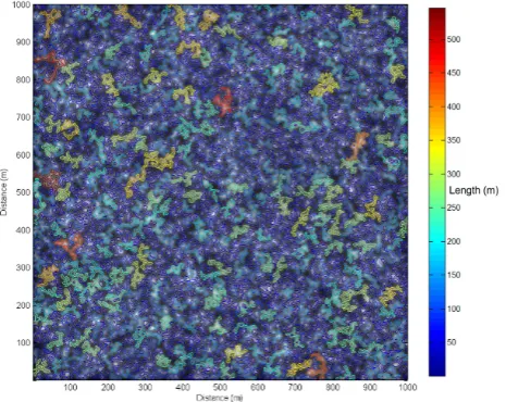
wherer2=(x2+y2). Hence the zero contour of the Lapla-cianL of the anomaly from a sphere will have a radius of z/2. Figure 1a shows a synthetic gravity dataset produced by a set of spheres. Their masses and depths are identical, and their locations are random. Their edges, as determined by the zero contour of the Laplacian, are plotted in Fig. 1b, and Fig. 1g shows the histogram of the edge contour lengths. Fig-ure 1 c, d, e, f show the plots obtained when different num-bers of spheres were used. The contour locations were deter-mined by linearly interpolating the Laplacian values of the data. When the spheres are few and relatively shallow then the overlap of anomalies is infrequent and the histogram has a prominent peak at a contour length ofπ.z, wherezis the depth of the spheres. However, as the number of spheres in-creases, their anomalies will interact more often and the his-togram shape becomes a power law. The presence of a power law in the behaviour of a system is a measure of its self-similarity, i.e. portions of an object look similar to the object itself, when suitably magnified. In this case, small contours have a similar appearance to large contours. Many objects in nature, such as clouds and trees, display fractal charac-teristics (Mandelbrot, 1982). This type of scale invariant be-haviour is exhibited by many geoscientific phemonema, such
288 G. R. J. Cooper: The scaling behaviour of the edges of gravity data
Fig. 1a. The gravity response from 100 000 point sources, each with a mass of 1011kg and a depth of 5 m.
Fig. 1b. Edge contours of the data shown in Fig. 1a. The contours are coloured according to their length.
as seismicity (Turcotte, 1997, p. 56), coastlines (Richardson, 1961), topography (Gagnon et al., 2006), faulting (Bohnen-stiehl and Kleinrock, 1999), and non-linear least-squares in-verse theory (Cooper, 2000). Fractal analysis has also been used to determine an optimum grid size in the interpolation of geophysical data (Dimri et al., 2005).
The fractal behaviour of a system is characterised by its fractal dimension, which is determined from the exponent of the power law that describes its behaviour in some manner. Customarily this is performed by taking logarithms of some measure of the data (in this case, the number of edge contours within a range of lengths is plotted against the mean value of
Fig. 1c, d. Histogram and log-log histogram of the lengths of the edge contours obtained from the gravity response from 10 000 sources at a depth of 5 m. A fitted power–law distribution is shown as a solid line.
tal dimension of the object or system. Figure 1i shows a plot of the fractal dimension obtained as a function of the number of spheres used. As more spheres are added their responses overlap more and hence the degree of spatial averaging of the gravity field gradually increases, the result eventually being a small number of relatively large contours. Boundary effects then become important as most contours intersect the spatial limits of the dataset. The statistics on the lengths of the con-tours then become unreliable and the power–law relationship breaks down. The shallower the sources are, the smaller their interaction and the greater the number of spheres required be-fore the breakdown occurs; conversely, the deeper they are, the lower the fractal dimension obtained and the smaller the number of spheres required to produce a breakdown in the power–law relationship.
grav-G. R. J. Cooper: The scaling behaviour of the edges of gravity data 289
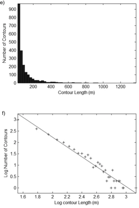
Fig. 1e, f. Histogram and log-log histogram of the lengths of the edge contours obtained from the gravity response from 50 000 sources at a depth of 5 m. A fitted power–law distribution is shown as a solid line.
up. Firstly, since each computation is essentially the same, one prior computation of the anomaly of a single source centred in a grid 2000×2000 points in size was made. In all, 1000×1000 point portions of this grid were then used when its centre was located randomly within the desired 1000×1000 point grid. Hence no repeated computations of the anomaly were made. Secondly, the computations were moved from the CPU to the GPU (nVidia GeForce GTX295) using the CUDA architecture. The time of computation was then reduced to a more reasonable 90 s.
Figure 1j shows the result of allowing the sphere masses to vary (randomly) as well as their location. The result is similar to that shown in Fig. 1i, although a higher fractal dimension is obtained. If the sphere depths are varied instead of their mass a similar behaviour was also observed.
Fig. 1g, h. Histogram and log-log histogram of the lengths of the edge contours in Fig. 1b. A fitted power–law distribution is shown as a solid line.
290 G. R. J. Cooper: The scaling behaviour of the edges of gravity data
Fig. 1j. Fractal dimension obtained as a function of the number of randomly located buried sphere sources, at a depth of 5 m. The mass of each sphere was generated randomly between 0 and 1011kg. Be-cause the fractal dimension depended on the locations of the spheres and these were calculated randomly, the experiment was repeated five times and the mean value and the standard deviation deter-mined.
3 The statistical distribution of the edges of a gravity dataset from South Africa
Figure 2a shows a Bouguer gravity dataset from South Africa. The image is 650 km×700 km in size, and the orig-inal approximately 90 000 gravity measurements (made by the Council for Geoscience, Pretoria) were gridded to a cell size of 1 km. The prominent circular anomaly on the middle right side is the Trompsburg high (Buchmann, 1960), and the Vredefort dome impact structure is just visible in the upper right corner of the figure. This portion of the South African gravity dataset was chosen because it is the largest rectangu-lar area that does not intersect South Africa’s borders, beyond which no data were available.
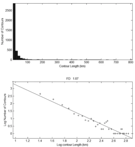
Figure 2b overlays the zero contours of the Laplacian on the gravity data, and Fig. 2c and d show the histogram of the edge contour lengths and a power-law fit. As suggested by the theoretical framework in the previous section, the scaling behaviour of the edges of the gravity data followed a power law, which had a fractal dimension of 1.87 for this particular area.
Fig. 2a. Gravity data over a portion of South Africa. The grid spac-ing is 1 km.
Fig. 2b. The gravity dataset from Fig. 2a is overlain by the zero contour of the Laplacian function. The contours are colour coded by their length.
4 Conclusions
G. R. J. Cooper: The scaling behaviour of the edges of gravity data 291
Fig. 2c, d. Histogram and log-log histogram of the lengths of the edge contours in Fig. 2b. A fitted power–law distribution is shown as a solid line.
Acknowledgements. The Council for Geoscience (Pretoria) is
thanked for permission to use the gravity dataset shown in Fig. 2. The NRF (Pretoria) is thanked for funding this project. The constructive comments of two anonymous reviewers helped to improve the manuscript.
Edited by: M. Fedi
Reviewed by: two anonymous referees
References
Bohnenstiehl, D. R. and Kleinrock, M. C.: Faulting and fault scal-ing on the median valley floor of the trans-Atlantic geotraverse (TAG) segment, 26◦N on the Mid-Atlantic Ridge, J. Geophys. Res., 104, 29351, 29531–29364, doi:10.1029/1999JB900256, 1999.
Buchmann, J. P.: Exploration of a geophysical anomaly at Tromps-burg, Orange Free State, South Africa, Trans. Geol. Soc. South Africa, 63, 1–10, 1960.
Cooper, G. R. J.: Fractal convergence properties of geophysical in-version, Comput. Graphics, 24, 603–609, 2000.
Dimri, V. P., Srivastava, R. P., and Vedanti, N.: Optimum gridding of potential field data: a case study, SEG Expanded Abstr. 24, 674, http://dx.doi.org/10.1190/1.2144413, 2005.
Gagnon, J.-S., Lovejoy, S., and Schertzer, D.: Multifractal earth topography, Nonlin. Processes Geophys., 13, 541–570, doi:10.5194/npg-13-541-2006, 2006.
Horn, B. K. P.: Hill shading and the reflectance map, Geo-Process., 2, 65–146, 1982.
Jahne, B.: Digital Image Processing, 6th edn, Springer, Berlin, 2005.
Mandelbrot, B.: The Fractal Geometry of Nature, W. H. Freeman & Co., 1982.
Richardson, L. F.: The problem of contiguity: An appendix to Statis-tic of Deadly Quarrels, in: General systems: Yearbook of the Society for the Advancement of General Systems Theory, (Ann Arbor, Mich.: The Society, [1956-: Society for General Systems Research) 6 (139), 139–187, 1961.