www.soil-journal.net/3/67/2017/ doi:10.5194/soil-3-67-2017
© Author(s) 2017. CC Attribution 3.0 License.
SOIL
A probabilistic approach to quantifying soil physical
properties via time-integrated energy and mass input
Christopher Shepard1, Marcel G. Schaap1, Jon D. Pelletier2, and Craig Rasmussen1
1Department of Soil, Water and Environmental Science, The University of Arizona, Tucson, AZ
85721-0038, USA
2Department of Geosciences, The University of Arizona, Tucson, AZ 85721-0077, USA
Correspondence to:Christopher Shepard ([email protected])
Received: 30 September 2016 – Discussion started: 18 October 2016 Revised: 16 February 2017 – Accepted: 5 March 2017 – Published: 30 March 2017
Abstract. Soils form as the result of a complex suite of biogeochemical and physical processes; however, effec-tive modeling of soil property change and variability is still limited and does not yield widely applicable results. We suggest that predicting a distribution of probable values based upon the soil-forming state factors is more effective and applicable than predicting discrete values. Here we present a probabilistic approach for quantify-ing soil property variability through integratquantify-ing energy and mass inputs over time. We analyzed changes in the distributions of soil texture and solum thickness as a function of increasing time and pedogenic energy (effective energy and mass transfer, EEMT) using soil chronosequence data compiled from the literature. Bivariate normal probability distributions of soil properties were parameterized using the chronosequence data; from the bivariate distributions, conditional univariate distributions based on the age and flux of matter and energy into the soil were calculated and probable ranges of each soil property determined. We tested the ability of this approach to predict the soil properties of the original soil chronosequence database and soil properties in complex terrain at several Critical Zone Observatories in the US. The presented probabilistic framework has the potential to greatly inform our understanding of soil evolution over geologic timescales. Considering soils probabilistically captures soil variability across multiple scales and explicitly quantifies uncertainty in soil property change with time.
1 Introduction
Pedogenic models that can be widely applied and easily uti-lized are paramount for understanding soil-landscape evo-lution, soil property change with time, and predicting fu-ture soil conditions. A mathematically simple, easily param-eterized approach has yet to be developed that is capable of predicting current soil properties or recreating potential soil evolution with time. Here we address this knowledge gap through the development of a probabilistic model of soil property change capable of predicting soil properties across a wide range of terrains, climates, and ecosystems.
The state-factor approach has been one of the primary pe-dogenic models since its development in the late 1800s and early 1900s (Dokuchaev, 1883; Jenny, 1941). The soil state-factor approach (Jenny, 1941) assumes that the state of the
Here we develop a simple probabilistic approach to pre-dict soil physical properties using a large dataset of chronose-quence studies. The model compresses state-factor variabil-ity into two key components (parent material and total pe-dogenic energy, defined in Sect. 1.1) that were parameter-ized and calibrated using the chronosequence database. We hypothesized that a probabilistic approach predicts accurate ranges of soil physical properties based on the soil-forming environment. Additionally, we modified the model to include soil depth to capture the influence of redistributive hillslope processes to predict soil properties. We hypothesized that by including soil depth, the model would effectively predict the clay content in an independent dataset synthesizing soil and landscape variability in complex, hilly terrain from a wide range of environments.
Probabilistic model of soil property change
The model presented here is based on a reformulated state-factor model, where a location has a probability of displaying a range of differing soil morphologies and properties based upon the state factors, with some range of values more prob-able than others, meaning that the state-factor model (Jenny, 1941) may be restated as
P(s1≤S≤s2)=f(cl, o, r, p, t), (1)
where the left-hand side of the equation, P(s1≤S≤s2),
represents the probability that a given soil will have a value located between a lower limit (s1) and an upper limit (s2)
(Phillips, 1993b). Equation (1) can be restated more simply as
P(s1≤S≤s2)=f(Lo, Px, t), (2)
where the original soil-forming state factors have been sim-plified to represent the fluxes of matter and energy into the soil system (Px), incorporating the influence of climate and biology, and the initial state of the soil-forming conditions (Lo), incorporating the influence of the initial topography and original soil parent material and time or age of the soil system (t) (Jenny, 1961).
Equation (2) was further simplified to make the approach operational. A quantitative measure of climate and biology was needed to represent the influence ofPx on soil forma-tion. We used a quantification ofPxcalculated from effective precipitation and biological productivity, termed effective en-ergy and mass transfer (EEMT, J m−2yr−1) (Rasmussen and Tabor, 2007; Rasmussen et al., 2005, 2011). EEMT provides a measure of the energy transferred to the subsurface, in the form of reduced carbon from primary productivity and heat transfer from effective precipitation, which has the poten-tial to perform pedogenic work, e.g., chemical weathering and carbon cycling. Using EEMT as a simplification ofPx, Eq. (2) was restated as (Rasmussen et al., 2011)
P(s1≤S≤s2)=f(Lo,EEMT, t). (3)
We further simplified Eq. (3) by combining the flux term EEMT and the age of the soil system (t). EEMT multiplied by the age of the soil system, i.e., EEMT×t, provides an es-timate of the total energy transferred to the soil system over the course of its evolution, referred to here as total pedogenic energy (TPE, J m−2). The TPE provides an estimate of Px that incorporates soil age; thus, Eq. (3) may be restated as
P(s1≤S≤s2)=f(Lo,TPE), (4)
where at a certain point in time the probability of a soil prop-erty existing betweens1ands2is a function ofLoand TPE. Locontrols the spread or variation of the probability distri-butionP(s1≤S≤s2) over time and the potential
observ-able soil states, whereas TPE is proportional to the internal soil state at a given time (Jenny, 1961). Explicitly includ-ing time in Eq. (4) through TPE partially captures variation in soil property change attributable to topography and par-ent material. Soil residence time may be directly related to landscape position through topographic control on soil pro-duction and sediment transport and deposition (Heimsath et al., 1997, 2002; Yoo et al., 2007). Additionally, parent ma-terial modulates soil residence time through control on soil depth (Heckman and Rasmussen, 2011; Rasmussen et al., 2005), soil production, and sediment transport rates (Andre and Anderson, 1961; Portenga and Bierman, 2011). The ini-tial conditions of the soil-forming system (Lo) are never fully known; however, representing the state of the soil system as a probable distribution of values, implicitly accounting for soil age, and not constraining the initial soil-forming conditions, the influence of initial conditions can be partially ignored, and hence we herein focus on modeling soil properties using only TPE.
Quantitatively realizing Eq. (4) required the use of pre-determined joint probability density functions parameterized with TPE and a selected soil physical property. Bivariate nor-mal density functions were calculated to determine the prob-ability of a soil property range given a TPE value. The bi-variate density function was selected due to its simplicity and ease of parameterization; other bivariate density func-tions are available that may better fit the selected soil prop-erty data but are not considered here. The bivariate normal density distribution (Ugarte et al., 2008) was calculated as
f(x, y)= 1 2π σxσy
p
1−ρ2exp −
1
2 1−ρ2 "
(x−µx)2
σ2
x
+ y−µy
2
σ2
y
−2ρ(x−µx) y−µy
σxσy
#!
, (5)
conditional means and variances parameterized conditional univariate normal distributions for the selected soil physical properties. The conditional mean (Ugarte et al., 2008) was calculated as
µY|X=x=µy+ρ σy σx
(x−µx), (6)
where µY|X=x is the conditional mean soil property value given a value for TPE. The conditional variance (Ugarte et al., 2008) was calculated as
σY2|X=x=σy21−ρ2, (7)
whereσY2|X=xis the conditional variance of the soil property given a value of TPE.
Applying this approach required certain assumptions and simplifications. The model assumes that climate was constant over the entire duration of pedogenesis. The model makes no assumptions about the progressive and regressive processes that drive pedogenesis; by weighting all profiles equally, the net effects of both progressive (e.g., horizonation, clay ac-cumulation, reddening) and regressive (e.g., haplodization, erosion, pedoturbation) pedogenic processes (Johnson and Watson-Stegner, 1987; Phillips, 1993a) are captured in the model structure. The model also does not consider the net ef-fect of progressive and regressive pedogenic processes on the distribution of selected soil properties with depth. The model makes no assumptions about the initial soil-forming system, and we did not constrain the model to any particular initial condition for either parent material or geomorphic landform; the model simply describes the probability of a location ex-hibiting a range of soil properties based on TPE. The model assumes that all changes in soil physical properties are due to pedogenic processes. We used a bivariate normal distribu-tion; consequently the model assumes that the data conform to a normal distribution.
2 Methods
2.1 Data collection and preparation
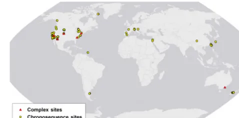
The probability distributions were parameterized using an extensive literature review of chronosequence studies. More than 140 chronosequence publications were identified us-ing Google Scholar (www.scholar.google.com) and Thom-son Reuters Web of Science (www.webofknowledge.com), 44 of which contained the required data. Inclusion within the present study required the following: profile descriptions with horizon-level clay, sand, and silt content and soil depth; well-defined ages of the soil-geomorphic surfaces; and ge-ographic coordinates or maps showing locations of the de-scribed profiles. The chronosequences spanned a wide range of geographic locations, ecosystems, climates, rock types, and geomorphic landforms (Fig. 1, Table S1 in the Supple-ment). The chronosequence soils spanned ages from 10 years
Figure 1.Map of study sites. Yellow points indicate location of chronosequences, and red triangles indicate location of soils in com-plex terrain.
to 4.35 Myr and depth ranges from 3.0 to 1460 cm, with mean annual temperature (MAT) and precipitation (MAP) ranging from−11.2 to 28.0◦C and 3.0 to 400 cm yr−1, respectively.
We were limited in site selection by the available data; as such we could not control for any bias that may exist with regard to site selection and reported soil property values.
2.2 Total pedogenic energy
2.3 Application to chronosequence data
The chronosequence database included 44 distinct chronose-quences representing 405 different soil profiles. We focused here on changes in sand, silt, and clay content and solum thickness as examples of soil property change with time. We tested the approach on depth-weighted (DWT) sand, silt, and clay content (reported as weight %), as well as the maximum measured value of sand, silt, and clay content within each soil profile. Buried horizons were removed from the soil pro-files before either the maximum or DWT content values were calculated. Solum thickness was extracted for each profile, defined as the thickness of the horizons influenced by pe-dogenic processes or the depth to C horizons (Schaetzl and Anderson, 2005). The site RW-14 from McFadden and Wel-don (1987) was not included in the solum thickness model calculations; the measured solum thickness of RW-14 was 1460 cm, 1 order of magnitude greater than all other soil pro-files included in the study. Four hundred and five propro-files reported clay content data, only 387 profiles reported sand and silt content, and 399 soil profiles contained a developed solum. We classified the soil profiles by parent material in terms of igneous, metamorphic, or sedimentary material and by geomorphic landform, e.g., alluvial surface, marine ter-race, or moraine (Shoeneberger et al., 2012); for example, if a soil was formed on an alluvial fan from granitic parent material, it would be defined as alluvial and igneous.
Using the soil data, we calculated bivariate normal prob-ability distributions using TPE and the soil physical prop-erties (Eq. 5). The soil data were transformed using loga-rithmic and square root transformations when appropriate to meet the normality assumption of the bivariate normal prob-ability distribution. Conditional univariate normal distribu-tions (Eqs. 6, 7) were calculated to approximate probable ranges of soil properties using leave-one-out cross validation (LOOCV). Each of the soil chronosequences was removed from the model dataset, with the all remaining chronose-quence data used to calculate the parameters of the bivariate and conditional univariate normal distributions. The condi-tional univariate normal distributions were calculated using the TPE values for the profiles within the left-out chronose-quence.
2.4 Application to complex terrain
By design, soil chronosequences are generally sited on gen-tle, low, sloping terrain to minimize the influence of topogra-phy and erosion/deposition on soil formation (Harden, 1982). However, much of the Earth’s surface is characterized by complex topography with high relief, steep slopes, and dif-ferences in slope aspect. Any predictive soil model or ap-proach must be effective in both simple and complex terrain. To test the ability of the model to predict soil properties in complex terrain, we compiled data from upland catchments with variable parent material and topography from the
lit-erature, as well as data available from the US NSF Criti-cal Zone Observatory Network (CZO, www.critiCriti-calzone.org) (Table 1) (Bacon et al., 2012; Dethier et al., 2012; Foster et al., 2015; Holleran et al., 2015; Lybrand and Rasmussen, 2015; Rasmussen, 2008; West et al., 2013). Data from several additional studies from complex terrain were also included to test the model (Table 1) (Dixon et al., 2009; Yoo et al., 2007). These data were accessed from www.criticalzone.org or Google Scholar (www.scholar.google.com). These stud-ies were included because they all contained horizon-level soil texture data, soil depth, percent volume rock fragment data, and10Be or U series measures of soil erosion rates or residence time, where mean residence time (MRT) was cal-culated as MRT=h/E, wherehis soil depth (m) andEis erosion rate (m yr−1) (Pelletier and Rasmussen, 2009b). We used published coordinates to extract EEMT values, calcu-lated from New et al. (1999), for each soil profile using Ar-cGIS 10.1 and used EEMT and MRT to calculate TPE. It should be noted the coarse resolution of New et al. (1999) EEMT values does not account for local-scale variation in water redistribution and primary productivity that can lead to significant topographic variation in EEMT (Rasmussen et al., 2015). Using Eq. (5) and the parameters generated from the chronosequence database, conditional mean depth-weighted clay content was calculated for each profile.
Due to the influence of redistributive hillslope processes on soil development (Yoo et al., 2007), soil depth varies sys-tematically across hillslopes (Heimsath et al., 1997); thus, soil depth can be used to incorporate information about these processes within the model calculations. We calculated the mass per area clay content of these profiles using soil depth to incorporate this variation, as
mass per area claykg m−2 (8)
=(ρb)(h)
µY|X=x,DWT CLAY
100
1−
RF%
100
,
whereρbis the soil bulk density assumed to be 1500 kg m−3
for all soil profiles,µY|X=x,DWT CLAYis the predicted
condi-tional mean for depth-weighted clay content (DWT CLAY) using Eq. (6), RF% is the measured depth-weighted percent volume rock fragments within the soil (when no RF% data were available we assumed a value of 41.7 %, which was the average RF% for profiles with reported values), andhis the soil depth in meters. Using Eq. (8), mass per area clay was calculated for each soil profile. Further, we examined the im-pact of depth, rock fragment percentage, and predicted con-ditional mean DWT clay on the predicted mass per area clay predictions using multiple linear regression.
Coupling geomorphic model with probabilistic model
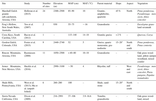
Table 1.Complex terrain study sites and characteristics.
Site Study Number
of sites
Elevation (m)
MAP (cm) MAT (◦C) Parent material Slope Aspect Vegetation
Marshall Gulch granite sub-catchment, Arizona, USA
Holleran et al. (2015)
24 2300–2500 85–90 10 Granite,
amphibolite, quartzite
45 % North Pinus ponderosa,
Pseudotsuga men-ziesii,Abies concolor
Frog’s Hollow, New South Wales, Australia
Yoo et al. (2007)
2 930 55–75 ∼16 Granodiorite – – Eucalyptus
grass-land savannah
Cross Keys, South Carolina, USA
Bacon et al. (2012)
1 – 115–140 14–18 Granitic gneiss < 2 % – Quercus, Carya
Gordon Gulch, Colorado, USA
Foster et al. (2015)
9 2440–2740 52 5 Gneiss, quartz
monzonite, gra-nodiorite
15–28◦ North
and south
Pinus ponderosa,
Pinus contorta
Rincon Mountains, Arizona, USA
Rasmussen (2008)
11 1050–2500 < 40–80 10–18 Granodiorite – – Oak grass
wood-land, piñon–juniper woodland, mixed conifer
Jemez Mountains, New Mexico, USA
Huckle et al. (2016)
4 2990–3100 ∼50 4 Rhyolite, tuff – West
and east
Pseudotsuga men-ziesii,Abies concolor, Picea
pungens,Populus tremuloides
Shale Hills, Pennsylvania, USA
West et al. (2013); Ma et al. (unpub-lished)
6 260–280 100 – Shale,
sand-stone
15–20◦ North
and south
–
Sierra Nevada California, USA
Dixon et al. (2009)
5 216–2991 37–106 3.9–16.6 Tonalite,
granodiorite
– – Oak-grass
wood-land, mixed conifer, subalpine
the Santa Catalina Mountains (Catalina-Jemez CZO, Fig. 2a– b, Table 1) (Holleran et al., 2015; Lybrand and Rasmussen, 2015). The ∼6 ha catchment is located at an elevation be-tween 2300 and 2500 m with mixed conifer vegetation, ap-proximately 30 km northeast of Tucson, AZ (Fig. 2, Table 1). The approach utilized soil depth and residence time output from a process-based numerical soil depth model (Pelletier and Rasmussen, 2009a). The model used high-resolution lidar-derived topographic data to estimate 2 m pixel reso-lution soil depth and erosion rates (Fig. 2c) (Pelletier and Rasmussen, 2009a). These data were coupled with topo-graphically resolved EEMT values that accounted for lo-cal hillslope-slo-cale variation in water redistribution and pri-mary productivity at a 10 m pixel resolution (Rasmussen et al., 2015) (Fig. 2d). We used calculated TPE from the to-pographically resolved EEMT and soil residence time values to predict DWT clay and coupled predicted DWT clay values with modeled depth from Pelletier and Rasmussen (2009a) in Eq. (8) to predict mass per area clay at a 2 m pixel resolution; the data processing and model apparatus are shown in Fig. 3. We assumed a constant 50 % rock fragment value for each location. The coupled geomorphic–TPE model outputs were compared with point measures of mass per area clay from
Holleran et al. (2015) and Lybrand and Rasmussen (2015). Model data were completely independent of the Holleran et al. (2015) and Lybrand and Rasmussen (2015) datasets such that they served as validation data for the modeled output.
2.5 Model domain
Figure 2.Marshall Gulch study site.(a)Location of the Santa Catalina Mountains and the Marshall Gulch catchment within Arizona, USA;
(b)elevation of the granite sub-catchment of Marshall Gulch;(c)predicted soil depth in the granite sub-catchment (Pelletier and Rasmussen, 2009a);(d)EEMTv2.0 in the granite sub-catchment (Rasmussen et al., 2015);(e)mismatch between the measured soil depths and predicted soil depths.
Process-based numerical soil depth model
Topographically resolved EEMT
model
Probabilistic soil property
model Soil depth
Soil residence
time
EEMT
Predicted DWT clay TPE
Eq. ( 9)
Mass per area clay
Figure 3.Coupled geomorphic–probabilistic model apparatus. The process-based numerical soil depth model is used to predict soil depth, which is used to predict soil residence time. The topographi-cally resolved EEMT model is used to calculate TPE using the soil residence time and EEMT values. The probabilistic model is used to calculate DWT clay contents using the TPE values, and mass per area clay is calculated using predicted DWT clay and predicted soil depth values.
3 Results
3.1 Application and parameterization to chronosequences
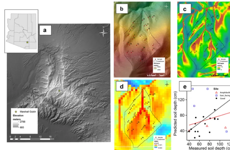
The relationships between TPE and soil texture and solum thickness were used to calculate the bivariate probability distributions. The bivariate probability distributions (Eq. 5) were parameterized using the means, standard deviations, and Pearson’s correlation from the chronosequence database (Table 2). Furthermore, the relationship between TPE and the soil properties was stronger than just using age, NPP, MAP, or MAT alone (Table 3). Age was expected to strongly cor-relate to the soil properties due to the design of chronose-quence studies; however, comparing age and TPE separately, the percent increase in Spearman rank correlations (r) ranged from 8.7 % (DWT silt) to 25.6 % (max sand). Maximum and depth-weighted silt content were weakly correlated to both age and TPE and exhibited only a minimal change in Spear-man’s rank correlation with TPE relative to age.
re-Table 2.Parameters for the bivariate normal probability distribu-tions for the soil physical properties and TPE;nis number of pro-files;µis mean;σ is standard deviation; andρis Pearson’s corre-lation between soil variables and total pedogenic energy.
Soil property parameters
Variable n µ σ ρ
Max sand 387 70.97 25.55 −0.48
Max silt 387 34.27 18.32 0.32
Max claya 405 4.52 2.26 0.78
DWT sand 387 59.47 26.22 −0.57
DWT silta 387 4.50 1.66 0.26
DWT claya 405 3.66 2.12 0.73
Solum thicknessb 399 1.77 0.53 0.65
TPEb 405c 8.69 1.30 –
387d 8.70 1.29 –
399e 8.72 1.27 –
aSquare root transformed.bLog10 transformed.cFor clay variables.dFor
sand and silt variables.eFor solum thickness, max indicates maximum
content; DWT indicates depth-weighted average content.
lated, but weaker relative to the maximum clay–TPE rela-tionship (Fig. S1 in the Supplement, Pearson’s ρ=0.65,
r2=0.42×log(solum thickness)= −0.58+0.27·log(TPE),
df=397). The relationships between TPE and max sand
(Fig. S2) and silt (Fig. S3) contents were generally weaker, relative to clay and solum thickness, with little to no relation-ship between TPE and silt content.
The conditional univariate normal distribution parameters were determined for the soil physical properties from the bi-variate distribution and using Eqs. (6) and (7). The bibi-variate normal distribution effectively predicted maximum clay con-tent (Fig. 5) with an r2=0.54 (RMSE=14.8 %) between the measured maximum clay content and predicted condi-tional mean maximum clay content (Eq. 6) across all sites based on LOOCV (Fig. 5d). The model effectively predicted maximum clay content regardless of parent material withr2
of 0.61 (RMSE=14.4 %), 0.56 (RMSE=12.0 %), and 0.59 (RMSE=16.8 %), for igneous, metamorphic, and sedimen-tary parent materials, respectively. Ther2between the mea-sured values and predicted values for solum thickness, max sand, and max silt were 0.28 (RMSE=101.0 cm, Fig. S4), 0.17 (RMSE=23.4 %, Fig. S5), and 0.04 (RMSE=18.0 %, Fig. S6), respectively.
The relationship of predicted to actual maximum clay content varied significantly across individual studies. The predicted values represent the predicted conditional means (Eq. 6) bounded by the conditional standard deviation (Eq. 7), which approximates a 50 % probability that the mea-sured maximum clay content will be within 1 standard devi-ation of the conditional mean (Fig. 6). The individual stud-ies presented in Fig. 6 were selected to represent a broad
0.02
0.04
0.06
0.08
6 8 10 12
0 2 4 6 8 10
6 8 10 12
0 2 4 6 8 10 Sqr t (maxim um cla
y content (%))
Log (total pedogenic energy (kJ m ))–2
● ● ● ● ●● ● ● ● ● ● ● ● ● ● ● ● ● ● ● ● ● ● ● ● ● ● ● ● ● ● ●●● ● ● ● ● ● ● ● ● ● ● ● ● ● ● ● ● ● ● ● ● ● ● ● ● ● ● ● ●● ● ● ● ● ● ● ● ● ● ● ● ● ● ● ● ● ● ● ● ● ● ● ● ● ● ● ● ● ● ●●● ● ● ● ● ● ● ● ● ● ● ● ● ● ● ● ● ● ● ● ● ● ● ● ● ● ● ● ● ● ● ● ● ● ● ●●●● ● ● ● ● ● ● ● ● ● ● ● ● ● ● ● ● ● ● ● ● ● ● ● ● ● ● ● ● ● ● ● ● ● ● ● ● ● ● ● ● ● ●● ● ● ● ● ● ● ● ● ● ● ● ● ● ● ● ● ● ● ● ●●● ●●● ● ● ● ● ● ● ● ● ● ● ● ● ● ● ● ● ● ● ● ●● ● ● ● ● ● ● ● ● ● ● ● ● ● ● ● ● ● ● ● ● ● ● ● ● ● ● ● ● ● ● ● ● ● ● ● ● ● ● ● ● ● ● ● ● ●● ● ● ● ● ● ● ● ● ● ● ● ● ● ● ● ● ● ●●● ● ● ● ● ● ● ● ● ● ● ● ● ● ● ● ● ● ● ● ● ● ●● ● ● ● ● ● ● ● ● ● ● ● ● ● ● ● ● ● ● ● ● ● ● ● ● ● ● ● ● ● ● ● ● ●● ●● ● ●● ● ● ● ● ● ● ● ● ● ● ● ● ● ● ● ● ● ● ● ● ● ● ● ● ●●●● ● ● ● ● ● ● ● ● ● ● ● ● ● ● ● ●●● ● ● ● ● ● ● ●● ●
Figure 4.Bivariate normal distribution between TPE and max clay content. The points indicate individual soils. The red ellipses rep-resent lines of equal probability, which corresponds to a three-dimensional probability distribution. From this relationship the con-ditional mean and variances for the soil physical properties were calculated.
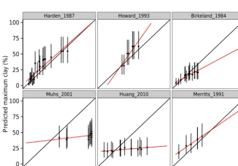
range of climates and landforms and demonstrate both the strengths and weaknesses of the model. For Harden (1987) (Fig. 6a,r2=0.88,p<0.0001, df=20, RMSE=9.4 %) and Howard et al. (1993) (Fig. 6b,r2=0.86,p<0.001, df=6, RMSE=10.2 %), the model was generally successful at pre-dicting the maximum clay content values; both the Harden (1987) and Howard et al. (1993) sequences were located in alluvial deposits but in vastly different climates: xeric (winter-dominated annual rainfall regime) vs. udic (evenly distributed annual rainfall regime), respectively. The model was capable of predicting maximum clay content values for glacial moraine deposits, in a frigid climate (Fig. 6c,r2= 0.87, p<0.0001, df=12, RMSE=6.0 % Birkeland, 1984) and on marine terraces in northern California with a xeric cli-mate (Fig. 6f,r2=0.98,p<0.001, df=4, RMSE=8.9 %; Merritts et al., 1991). The model was incapable of predict-ing clay accumulation on marine terraces in hot, wet cli-mates in Barbados (Fig. 6d, r2=0.31, p=0.08, df=9, RMSE=44.9 % Muhs, 2001) or Taiwan (Fig. 6e,r2=0.67,
p<0.001, df=11, RMSE=23.1 %, Huang et al., 2010).
3.2 Application in complex terrain
The model was much less effective in complex terrain and highly overpredicted DWT clay contents in soils located in complex landscapes (Fig. 7a,r2=0.26, y=0.39x+7.36,
Igneous Metamorphic Sedimentary (All)
0 25 50 75 100
0 25 50 75 100 0 25 50 75 100 0 25 50 75 100 0 25 50 75 100
Measured maximum clay content (%)
P
re
d
ic
te
d
ma
x
im
u
m
cl
a
y
co
n
te
n
t (
%
)
50 000 100 000 150 000 200 000
EEMT (kJ m−2 yr−1)
Landform
Alluvial Anthropogenic Beach ridges Coral reef terrace Dunes Floodplain Fluvial terrace Glacial moraine Lake terrace Lateritic Marine terrace Paleochannel Uplands Volcanic
Figure 5.LOOCV results for max clay content. The results were subdivided by general soil parent material: igneous, metamorphic, and sedimentary; the points represent the geomorphic surface each soil formed on, and the colors represent the EEMT value for the location of each soil. Using LOOCV, where one chronosequence was removed from the model dataset and the remaining datasets were used to predict the parameters of the bivariate distributions, the conditional means of the left-out chronosequence was determined. The model was effectively able to predict the conditional mean values of the max clay contents with anr2=0.54 (RMSE=14.8 %). The model was least capable of predicting the clay contents on coral reef terraces (+) and appeared the most effective for alluvial surfaces ().
Harden_1987 Howard_1993 Birkeland_1984
Muhs_2001 Huang_2010 Merritts_1991 0
25 50 75 100
0 25 50 75 100
0 25 50 75 100 0 25 50 75 100 0 25 50 75 100 Measured maximum clay (%)
P
re
d
ic
te
d
ma
x
im
u
m
cl
a
y
(
%
)
Figure 6.Selected relationships between the measured maximum clay content and predicted maximum clay content. (a) Harden (1987),(b)Howard et al. (1993),(c)Birkeland (1984),(d)Muhs (2001),(e)Huang et al. (2010), and(f)Merritts et al. (1991). The er-rors represent the conditional standard deviations around the mean, which correspond to a probability of 50 %. The model effectively predicted clay content across a diverse range of climates, landforms, and parent materials. The model was the least effective at predict-ing the clay content of soils in tropical climates and soils formpredict-ing on coral reef terraces.
When correcting for the influence of hillslope processes by explicitly including soil depth and calculating mass per area clay, the approach effectively predicted clay content, with an r2=0.81 (Fig. 7b, y=1.58x−15.5, p<0.0001, RMSE=86.4 kg clay m−2), only slightly overpredicting clay
content, with a regression slope of 1.58. Soil depth was the strongest contributing factor to the mass per area clay pre-diction with the greatest sums of squares in a simple multi-ple linear regression including depth, RF%, and DWT clay% (Table 4); predicted conditional mean clay content percent-age was the second strongest contributing factor to the mass per area clay prediction. Rock fragment percentage did not influence the mass per area clay content prediction.
3.3 Coupled geomorphic–TPE model
The coupled geomorphic–TPE model effectively predicted mass per area clay for the majority of soils located within the Marshall Gulch sub-catchment with anr2=0.74 (Fig. 8a,
y=0.86x−5.06, p<0.0001, RMSE=17.7 kg clay m−2).
Figure 7.Model results in complex terrain.(a)Prediction of depth-weighted (DWT) clay contents;(b)prediction of mass per area clay using Eq. (9). The model was incapable of directly predicting DWT clay for the soils in complex terrain due to redistributive hillslope processes;r2=0.26 between measured and predicted conditional mean DWT clay(a). By including information about soil depth and percent volume rock fragment and converting DWT clay to mass per area clay, the model was significantly more effective at predicting clay contents for these soilsr2=0.81.
4 Discussion
4.1 Model effectiveness
4.1.1 Model results for chronosequences
The model predicted maximum clay content across a di-verse range of lithologies, climates, and landforms. Weath-ering and clay production are primary pedogenic processes (Birkeland, 1999; Schaetzl and Anderson, 2005), and be-cause the model assumed that all changes in the soil pro-file are due to these processes and TPE is closely related to degree of weathering, the model was the most effective at predicting clay content. For initial soil states that begin
Figure 8. Model results of coupled geomorphic–EEMT–TPE model in Marshall Gulch granite sub-catchment.(a)Prediction of mass per area clay for sites from Holleran et al. (2015) and Lybrand and Rasmussen et al. (2015);(b)spatial prediction of mass per area clay. When combining the present approach, with a geomorphic-based soil depth model, the combined models together were highly effective at predicting the clay contents for a majority of soils in the Santa Catalina Mountains (Catalina-Jemez CZO),r2=0.74.
environ-ments (Maejima et al., 2005; Muhs, 2001). Coral reef ter-races represent a relatively unique landform that weathers rapidly to fine-sized particles, especially under tropical cli-mates, and generally have complicated parent material com-positions (Muhs et al., 1987). The combination of these fac-tors limited the ability of the model to predict the soil prop-erties on these surfaces.
Sand and silt displayed weaker relationships with increas-ing total pedogenic energy. The lack of correlation of sand and silt to TPE may result in part from the definitions of the particle size classes. Sand-sized particles span a difference in particle size of several orders of magnitude, ranging from particles of 2 to 0.05 mm (Soil Survey Staff, 2010), whereas clays are constrained to a particle size less than 0.002 mm. The sequential weathering of rock fragments and coarse sand to fine and very fine sands therefore is not reflected in total sand content and likely diminishes the relationship between sand content and total pedogenic energy and time (Pye and Sperling, 1983; Pye, 1983; Sharmeen and Willgoose, 2006). The relationship between silt content and pedogenic energy was the weakest of the three broad particles size classes (Ta-bles 2, 3). Similar to sand, the silt size fractions span 1 order of magnitude in particle size ranging from 0.05 to 0.002 mm in diameter. Further, the sand and silt fractions are domi-nated by resistant primary minerals (Pye, 1983) and would not change greatly in response to increased TPE or weath-ering, which may partly account for the weaker correlations with TPE. Additionally, the silt fraction may also be heavily influenced by the deposition of eolian material and thereby introduce an additional mass of silt that was not derived from the direct weathering of the initial soil-forming system (Mc-Fadden et al., 1987) effectively uncoupling silt content from total pedogenic energy.
Solum thickness displayed a relatively strong relationship with increasing pedogenic energy, with TPE explaining up to 42 % of the variance in solum thickness (Tables 2, 3). Soil production is related to climatic variation (Amundson et al., 2015), with this variation partly captured by EEMT and TPE, leading to the slightly stronger predictive power of the model. However, soil production is also highly influenced by redis-tributive hillslope process, chemical and physical weather-ing, and tectonic uplift (Heimsath et al., 1997; Riebe et al., 2004; Yoo and Mudd, 2008b) and can be a highly nonlin-ear process (Pelletier and Rasmussen, 2009a). These factors were not directly accounted for in this study in that topog-raphy was not a quantified factor, which likely represents a large proportion of the remaining unexplained variance in solum thickness.
4.1.2 Model results in complex terrain
Due to using soil chronosequence data to parameterize the approach, the influence of redistributive hillslope processes was not captured. Additionally, in the amount of time re-quired to transport soil across a hillslope, chemical and
phys-ical alterations of the soil particles are possible and may not be reflected in mean residence time calculations (Yoo and Mudd, 2008a; Yoo et al., 2007). Soil thickness is highly de-pendent upon hillslope position and landscape morphology (Dietrich et al., 2003; Heimsath et al., 1997; Pelletier and Rasmussen, 2009a). By using soil thickness as a proxy for the strength of these redistributive hillslope processes and converting the predicted conditional mean clay content value to a mass per area basis, the model was able to capture differ-ences in clay content across complex terrain for a variety of lithologies and climates. The differing lithologies, climates, or vegetation types did not appear to impact the ability of the model to predict clay contents, likely because local varia-tion in soil depth accounts for many of these controls. Parent material and climate influence the weathering process and production of clay in soils (Harden and Taylor, 1983; Muhs et al., 2001); however, these factors are collinear with soil depth (Heckman and Rasmussen, 2011; Lybrand and Ras-mussen, 2015; Pelletier and RasRas-mussen, 2009a), such that by including soil depth, differences due to lithology or climate were partly incorporated in the model prediction.
4.1.3 Results from coupled geomorphic–TPE model
For the majority of sites in the Marshall Gulch sub-catchment, the coupled geomorphic–TPE model was highly effective at predicting clay content and the spatial distribu-tion of clay stocks. Large differences were found for four soils located on the east-facing ridge of the catchment under-lain by granite, with the model generally overpredicting soil depth and clay content. Discrepancies between the modeled and measured depths were likely the primary sources of error within the mass per area clay predictions for the four east-facing ridge soils (Fig. 2e). The geomorphic model predicted deeper soil depths due to the presence of an apparent con-vergent zone on the east-facing ridge of the sub-catchment; however, this convergent zone is only a small feeder tribu-tary to the larger catchment drainage. The inability of the model to effectively predict clay contents and the mismatch between modeled and actual soil depths in the four soils lo-cated on the east-facing ridge is likely due to this local, fine-scale topographic variation. The fine-fine-scale topographic vari-ation may indicate that the scale of soil property predictions is important in achieving accurate predictions. Fine spatial scales match the scale of local soil-landscape variation and processes, but fine-scale variation in weathering rates and lithology is also required to better predict soil depth within the catchment (McKenzie and Ryan, 1999).
Ras-Table 3.Spearman rank correlations between soil physical properties and TPE and age.
Spearman rank correlations
Variable NPP MAP MAT TPE Age % increase∗ n
Max sand −0.34 −0.15 −0.23 −0.46 −0.36 25.6 387
Max silt 0.00 −0.11 0.05 0.31 0.32 −1.1 387
Max clay 0.16 −0.01 0.37 0.80 0.73 8.8 405
DWT sand −0.25 −0.07 −0.27 −0.57 −0.50 15.2 387
DWT silt 0.11 −0.01 0.02 0.23 0.21 8.7 387
DWT clay 0.22 0.02 0.40 0.75 0.67 11.7 405
Solum thickness 0.12 0.07 0.22 0.63 0.58 9.9 399
Max indicates maximum content; DWT indicates depth-weighted average content;∗percent increase in Spearman
rank correlation between TPE and age.
Table 4.Sensitivity analysis of model prediction in complex terrain.
Sensitivity analysis of model prediction in complex terrain
Effects DF Sums of squares Mean sums of squares Fvalue p
Depth,h(cm) 1 1 158 897 1 158 897 472.9 <0.0001
CM DWT clay,µY|X=x(%) 1 148 896 148 896 60.8 <0.0001
Rock fragment, RF% (%) 1 1563 1563 0.6 0.428
Residuals 58 142 140 2451
mussen, 2009a); due to differences in primary mineral as-semblage, the amphibolite materials are likely weathering at a faster rate compared to the granite-derived soils (White et al., 2001; Wilson, 2004), resulting in greater clay produc-tion and likely explaining the underestimated clay contents. Inclusion of differential weathering rates for varying litholo-gies within the geomorphic model would likely lead to better prediction of clay contents, but in areas of complex lithology this would require detailed information about distributions of differing lithologies. With these adjustments, the coupled geomorphic–TPE model represents an effective, independent prediction of clay stocks.
4.2 Advantages of probabilistic approach
Simplifying and representing the soil-forming factors as mul-tivariate distributions and probabilities has the potential to quantitatively represent the general state-factor model, mak-ing the approach universally applicable. The initial state of the soil can likely never be fully known, leading to variability in soil properties over time that cannot necessarily, or ever, be attributed to any external factor (Phillips, 1989, 1993b). A probabilistic approach utilizes that variability to drive predic-tions and understanding of these systems. Similar to the ap-proach taken here, building distributions of the soil-forming state factors that are associated with distributions of partic-ular soil properties could yield probabilistic predictions of soil formation and change. We selected to use a represen-tation of climate and biology (EEMT). However,
depend-ing on the soil property of interest, the variables needed to parameterize the distributions would likely change; for ex-ample, if interested in organic matter content, aboveground net primary productivity or the normalized difference vege-tation index may be better predictors of organic matter accu-mulation. The strength of this approach lies in the fact that no assumptions are made about the initial conditions of the soil-forming system or the specific soil-forming processes. Predicting probable distributions of soil physical properties implicitly acknowledges that our understanding of any sys-tem is incomplete but explicitly quantifies uncertainty in pre-dictions and constrains the potential observable values to a predicted range. Utilizing this approach will require the necessary data to build distributions that are widely repre-sentative and applicable to most locations (Yaalon, 1975). With wide accessibility to large databases of soil informa-tion, such as the US National Soil Information System (NA-SIS) and the FAO Harmonized World Soil Database, access to the required amount and quality of data may be possi-ble. Similar to the present study, simple bivariate distribu-tions could be solved to calculate conditional distribudistribu-tions based on the soil-forming state factors, effectively producing quantitative probabilistic representations of Jenny’s original equation (Jenny, 1941).
on producing hypothetical soil-landscape relationships that progress forward through time (Minasny and McBratney, 2001; Vanwalleghem et al., 2013) or have focused on ide-alized landscapes (Temme and Vanwalleghem, 2015). How-ever, by combining probabilistic approaches parameterized using known landscapes and geomorphically based land-scape evolution models, predictions of the current state of the soil landscape can be investigated. As was demonstrated in Fig. 7b, combining the present approach with geomor-phically based soil depth models generated from DEMs has great potential to predict soil properties across a diverse range of environments, without needing prior knowledge of the landscape other than topography and climate. Further, potential soil landscapes can be investigated by updating EEMT values to incorporate future climate scenarios avail-able from predictive climate models (Gent et al., 2011; Tay-lor et al., 2012) and topographic and hydrological impacts due to changes in topography over time (Rasmussen et al., 2015).
4.3 Limitations and potential refinements
There are obvious limitations within the current model: a lack of consideration of parent material influences, topo-graphic variation, human impacts, internal soil feedbacks and thresholds, determination of landscape and soil age, and dif-ferences in paleoclimate variation. Parent material control on the relative proportion of weatherable minerals and mineral weathering rates (Jackson et al., 1948) can manifest itself as vastly different soil morphologies and rates of pedogenesis when controlling for other soil-forming factors or even with-out controlling for other factors (Heckman and Rasmussen, 2011; Parsons and Herriman, 1975; Phillips, 1993b). The current approach implicitly assumes no information about the initial conditions, only that all clay production is a pe-dogenic process. The application of this approach to par-ent materials, where a large fraction of clay-sized particles formed through non-pedogenic processes, is thus limited and may explain why the model was ineffective for some soils. Refining the current approach would require normalization of soil to the particle size distribution of the soil parent ma-terial. Past studies have utilized highly characterized parent material data to model soil property change with time (Chad-wick et al., 1990; Harden, 1982), but these data are gener-ally difficult to obtain and often not reported in the available chronosequence literature.
Topography dictates soil chemical and physical proper-ties and residence times, especially in complex terrain (Al-mond et al., 2007; Egli et al., 2008; Lybrand and Rasmussen, 2015), where nonlinear diffusive hillslope processes control the fluxes of matter and energy into and out of the soil sys-tem (Heimsath et al., 1997; Pelletier and Rasmussen, 2009a; Rasmussen et al., 2015; Yoo and Mudd, 2008b; Yoo et al., 2007). Using earlier versions of EEMT (Rasmussen and Ta-bor, 2007; Rasmussen et al., 2005), the current formulation
of the model and TPE does not explicitly quantify topo-graphic variation, which may account for error within cur-rent soil property distributions and predictions. With the in-clusion of topographic variation in EEMT (Rasmussen et al., 2015) and topographic control of soil residence times (Foster et al., 2015; West et al., 2013), we were able to correct this error with the present approach and effectively predicted clay stocks in complex terrain.
Human activities significantly alter soil physical proper-ties (Grieve, 2001; Neff et al., 2005; Pouyat et al., 2007). For example, differences in land use and increased grazing activity can alter soil physical properties such as clay and sand content across landscapes (Neff et al., 2005; Pouyat et al., 2007) or compaction from farming equipment leading to increased bulk density and increased erosion rates (Fullen, 1985; Hamza and Anderson, 2005). Human impacts on soil physical properties were not included in the presented model. The energetic contributions due to human impacts can be in-corporated within the EEMT apparatus, and adjusted model parameters can be calculated (Rasmussen et al., 2011). Hu-man impacts on soil physical properties may be locally im-portant, but for the majority of locations, human energetic contributions to the soil system are generally orders of mag-nitude smaller compared to the energetic inputs from solar radiation, precipitation, or primary productivity.
Internal or intrinsic feedbacks and thresholds within the soil system drive pedogenic development without changes in the external state factors (Chadwick and Chorover, 2001; Muhs, 1984). For example, greater chemical weathering and clay production due to increased water residence time caused by argillic horizon development is the result of an internal feedback that is independent of the external climatic and bio-logical system (Schaetzl and Anderson, 2005). These thresh-olds can operate as progressive or regressive processes, driv-ing soil formation forward or hinderdriv-ing further development (Johnson and Watson-Stegner, 1987; Phillips, 1993a). In-ternal soil development feedbacks were not explicitly con-sidered in the present model formulation. The presence of these internal feedbacks may partially explain error within the model predictions. Changes in EEMT would not explain all observed differences in soil properties over the age of the soil. However, if these feedbacks were operating in the in-cluded soils, the influence of intrinsic thresholds was implic-itly captured within the probability distributions, partially ac-counting for the role of internal soil development feedbacks on soil formation.
relative-age dating methods using landscape position are easily uti-lized and can provide the necessary age constraint needed to make model predictions (Burke and Birkeland, 1979; Favilli et al., 2009; Huggett, 1998; Matthews and Shakesby, 1984; Nicholas and Butler, 1996; Schaetzl and Anderson, 2005). Age constraint may also be achieved using landscape or hill-slope morphology derived from elevation transects or digital elevation models to estimate a “diffusivity age” for the soil (Hsu and Pelletier, 2004; Pelletier et al., 2006).
Global climate patterns have shifted dramatically over the last 65 Myr (Zachos et al., 2001). The majority of soils ob-served in the compiled chronosequence database span the Quaternary, including both the Holocene and Pleistocene. The Pleistocene was marked by a number of major glacial-interglacial cycles at approximately 100 000-year intervals (Imbrie et al., 1992; Wallace and Hobbs, 2006), which cor-responded with shifting climatic conditions; e.g., for large portions of the northern midlatitudes glacial periods were generally cooler and wetter and interglacial periods were warmer and drier (Connin et al., 1998; Petit et al., 1999). Fur-ther, the Pleistocene climate shifts likely influenced the rates of weathering and clay production (Hotchkiss et al., 2000). Taking into account the differences in past and modern cli-mate would partially reduce prediction errors between ob-served and modeled soil physical properties. Reconstructed global paleo-EEMT values would improve model accuracy and limit uncertainty in the probabilistic ranges of soil prop-erties for soils older than Holocene age.
5 Conclusions
The present approach effectively predicts soil physical prop-erties across a diverse range of geomorphic surfaces, litholo-gies, ecosystems, and climates. Further, this approach is mathematically simple and only requires knowledge of the probable age of a geomorphic surface and the effective en-ergy and mass transfer value associated with a given location, making this approach universally applicable. The simplicity of the probabilistic approach lies in the lack of the need to consider the initial conditions of the soil-forming state or the processes driving soil property change. A probabilistic approach does not exactly predict a soil physical property value at a given location but constrains the probable values based upon the state of the external environment to the soil. Using probabilistic approaches, we can model probable soil-landscape evolution scenarios, greatly informing our under-standing of the evolution of critical zone structure.
Data availability. All of the data used in this study can be found in the published studies in Table 1 and Supplement Table 1.
The Supplement related to this article is available online at doi:10.5194/soil-3-67-2017-supplement.
Competing interests. The authors declare that they have no con-flict of interest.
Acknowledgements. We thank Molly Holleran, Rebecca Ly-brand, and Ashlee Dere for providing data for this study. Support for C. Shepard was provided by the University Fellows program at the University of Arizona and by the University of Arizona/NASA Space Grant Graduate Fellowship. This research was funded by the US National Science Foundation grant no. EAR-1331408 provided in support of the Catalina-Jemez Critical Zone Observatory. Lidar data acquisition was supported by US National Science Foundation grant no. EAR-0922307 (P. I. Qinghua Guo).
Edited by: P. Finke
Reviewed by: J. Phillips and one anonymous referee
References
Almond, P., Roering, J., and Hales, T. C.: Using soil resi-dence time to delineate spatial and temporal patterns of tran-sient landscape response, J. Geophys. Res., 112, F03S17, doi:10.1029/2006JF000568, 2007.
Amundson, R., Heimsath, A., Owen, J., Yoo, K., and Dietrich, W. E.: Hillslope soils and vegetation, Geomorphology, 234, 122– 132, doi:10.1016/j.geomorph.2014.12.031, 2015.
Anderson, R. S., Repka, J. L., and Dick, G. S.: Explicit treatment of inheritance in dating depositional surfaces using in site 10Be and 26Al, Geology, 24, 47–51, 1996.
Andre, J. and Anderson, H.: Variation of Soil Erodibility with Geology, Geographic Zone, Elevation, and Vegetation Type in Northern California Wildlands, J. Geophys. Res., 66, 3351–3358, 1961.
Bacon, A. R., Richter, D. D., Bierman, P. R., and Rood, D. H.: Cou-pling meteoric 10Be with pedogenic losses of 9Be to improve soil residence time estimates on an ancient North American in-terfluve, Geology, 40, 847–850, doi:10.1130/G33449.1, 2012. Bierman, P. R.: Using in situ produced cosmogenic isotopes
to estimate rates of landscape evolution: A review from the geomorphic perspective, J. Geophys. Res., 99, 13885–13896, doi:10.1029/94JB00459, 1994.
Birkeland, P. W.: Holocene soil chronofunctions, Southern Alps, New Zealand, Geoderma, 34, 115–134, doi:10.1016/0016-7061(84)90017-X, 1984.
Birkeland, P. W.: Soils and Geomorphology, Third., Oxford Univer-sity Press, New York, New York, 1999.
Burke, R. M. and Birkeland, P. W.: Reevaluation of multiparameter relative dating techniques and their application to the glacial se-quence along the eastern escarpment of the Sierra Nevada, Cali-fornia, Quat. Res., 11, 21–51, doi:10.1016/0033-5894(79)90068-1, 1979.
Chadwick, O. A. and Chorover, J.: The chemistry of pedo-genic thresholds, Geoderma, 100, 321–353, doi:10.1016/S0016-7061(01)00027-1, 2001.
Connin, S., Betancourt, J., and Quade, J.: Late Pleistocene C4 plant dominance and summer rainfall in the southwestern United States from isotopic study of herbivore teeth, Quat. Res., 50, 179–193, 1998.
Dethier, D. P., Birkeland, P. W., and McCarthy, J. A.: Using the accumulation of CBD-extractable iron and clay content to estimate soil age on stable surfaces and nearby slopes, Front Range, Colorado, Geomorphology, 173–174, 17–29, doi:10.1016/j.geomorph.2012.05.022, 2012.
Dietrich, W. E., Bellugi, D. G., Heimsath, A. M., Roering, J. J., Sklar, L. S., and Stock, J. D.: Geomorphic Transport Laws for Predicting Landscape Form and Dynamics, Geophys. Monogr., 135, 1–30, doi:10.1029/135GM09, 2003.
Dixon, J. L., Heimsath, A. M., and Amundson, R.: The crit-ical role of climate and saprolite weathering in landscape evolution, Earth Surf. Process. Landforms, 34, 1507–1521, doi:10.1002/esp.1836, 2009.
Dokuchaev, V. V.: Russian Chernozem, edited by S. Monson, Israel Program for Scientific Translations Ltd. (For USDA-NSF), 1967 (Translated from Russian to English by N. Kaner), Jerusalem, Israel, 1883.
Egli, M., Merkli, C., Sartori, G., Mirabella, A., and Plotze, M.: Weathering, mineralogical evolution and soil organic matter along a Holocene soil toposequence developed on
carbonate-rich materials, Geomorphology, 97, 675–696,
doi:10.1016/j.geomorph.2007.09.011, 2008.
Favilli, F., Egli, M., Brandova, D., Ivy-Ochs, S., Kubik, P., Cheru-bini, P., Mirabella, A., Sartori, G., Giaccai, D., and Haeberli, W.: Combined use of relative and absolute dating techniques for detecting signals of Alpine landscape evolution during the late Pleistocene and early Holocene, Geomorphology, 112, 48–66, doi:10.1016/j.geomorph.2009.05.003, 2009.
Finke, P. A.: Modeling the genesis of luvisols as a function of topo-graphic position in loess parent material, Quat. Int., 265, 3–17, doi:10.1016/j.quaint.2011.10.016, 2012.
Foster, M. A., Anderson, R. S., Wyshnytzky, C. E., Ouimet, W. B., and Dethier, D. P.: Hillslope lowering rates and mobile-regolith residence times from in situ and meteoric 10 Be analysis, Boul-der Creek Critical Zone Observatory, Colorado, Geol. Soc. Am. Bull., 127, 862–878, doi:10.1130/B31115.1, 2015.
Fullen, M. A.: Compaction, hydrological processes and soil erosion on loamy sands in east Shropshire, England, Soil Tillage Res., 6, 17–29, doi:10.1016/0167-1987(85)90003-0, 1985.
Gent, P. R., Danabasoglu, G., Donner, L. J., Holland, M. M., Hunke, E. C., Jayne, S. R., Lawrence, D. M., Neale, R. B., Rasch, P. J., Vertenstein, M., Worley, P. H., Yang, Z. L., and Zhang, M.: The community climate system model version 4, J. Clim., 24, 4973– 4991, doi:10.1175/2011JCLI4083.1, 2011.
Gosse, J. C. and Phillips, F. M.: Terrestrial in situ cosmogenic nu-clides: theory and application, Quat. Sci. Rev., 20, 1475–1560, doi:10.1016/S0277-3791(00)00171-2, 2001.
Granger, D. E. and Muzikar, P. F.: Dating sediment burial with in situ-produced cosmogenic nuclides: Theory, tech-niques, and limitations, Earth Planet. Sci. Lett., 188, 269–281, doi:10.1016/S0012-821X(01)00309-0, 2001.
Grieve, I. C.: Human impacts on soil properties and their implica-tions for the sensitivity of soil systems in Scotland, Catena, 42, 361–374, doi:10.1016/S0341-8162(00)00147-8, 2001.
Hamza, M. A. and Anderson, W. K.: Soil compaction in cropping systems: A review of the nature, causes and possible solutions, Soil Tillage Res., 82, 121–145, doi:10.1016/j.still.2004.08.009, 2005.
Harden, J.: A quantitative index of soil development from field de-scriptions: Examples from a chronosequence in central Califor-nia, Geoderma, 28, 1–28, 1982.
Harden, J.: Soils Developed in Granitic Alluvium near Merced, Cal-ifornia, USGS Bulletin 1590-A, Washington, DC, 1987. Harden, J. W. and Taylor, E. M.: A quantitative comparison of Soil
Development in four climatic regimes, Quat. Res., 20, 342–359, doi:10.1016/0033-5894(83)90017-0, 1983.
Heckman, K. and Rasmussen, C.: Lithologic controls on regolith weathering and mass flux in forested ecosys-tems of the southwestern USA, Geoderma, 164, 99–111, doi:10.1016/j.geoderma.2011.05.003, 2011.
Heimsath, A. M., Dietrich, W. E., Nishiizumi, K., and Finkel, R. C.: The soil production function and landscape equilibrium, Nature, 388, 358–361, 1997.
Heimsath, A. M., Chappell, J., Spooner, N. A., and Questiaux, D. G.: Creeping soil, Geology, 30, 111, doi:10.1130/0091-7613(2002)030<0111:CS>2.0.CO;2, 2002.
Holleran, M., Levi, M., and Rasmussen, C.: Quantifying soil and critical zone variability in a forested catchment through digi-tal soil mapping, SOIL, 1, 47–64, doi:10.5194/soil-1-47-2015, 2015.
Hotchkiss, S., Vitousek, P. M., Chadwick, O. A., and Price, J.: Cli-mate Cycles, Geomorphological Change, and the Interpretation of Soil and Ecosystem Development, Ecosystems, 3, 522–533, doi:10.1007/s100210000046, 2000.
Howard, J., Amos, D., and Daniels, W.: Alluvial soil chronose-quence in the Inner Coastal Plain, Virginia, Quat. Res., 39, 201– 213, 1993.
Hsu, L. and Pelletier, J. D.: Correlation and dating of Quaternary alluvial-fan surfaces using scarp diffusion, Geomorphology, 60, 319–335, doi:10.1016/j.geomorph.2003.08.007, 2004.
Huang, W.-S., Tsai, H., Tsai, C.-C., Hseu, Y., and Chen, Z.-S.: Subtropical Soil Chronosequence on Holocene Marine Ter-races in Eastern Taiwan, Soil Sci. Soc. Am. J., 74, 1271, doi:10.2136/sssaj2009.0276, 2010.
Huckle, D., Ma, L., McIntosh, J., Vazquez-Ortega, A., Rasmussen, C., and Chorover, J.: U-series isotopic signatures of soils and headwater streams in a semi-arid complex volcanic terrain, Chem. Geo., 445, 68–83, doi:10.1016/j.chemgeo.2016.04.003, 2016.
Huggett, R. J.: Soil chronosequences, soil development, and soil evolution: a critical review, Catena, 32, 155–172, doi:10.1016/S0341-8162(98)00053-8, 1998.
Imbrie, J., Boyle, I. E. A., Clemens, S. C., Duffy, A., Howard, I. W. R., Kukla, G., Kutzbach, J., Martinson, D. G., Mclntyre, A., Mix, A. C., Molfino, B., Morley, J. J., Pisias, N. G., Prell, W. L., Peterson, L. C., and Toggweiler, J. R.: On the structure and ori-gin of major glaciation cycles 1. Linear responses to Milankovith forcing, Paleoceanography, 7, 701–738, 1992.
Jenny, H.: Factors of Soil Formation: A System of Quanti-tative Pedology, Dover Publications, Inc, New York, New York, available at: http://books.google.com/books?hl=en&lr= &id=orjZZS3H-hAC&oi=fnd&pg=PP1&dq=Factors+of+ Soil+Formation:+A+System+of+Quantitative+Pedology&ots=
fIfMb5fWkk&sig=e6Ev-CJjgsMYaO8DzFszbQK6Sss (last
access: 6 November 2014), 1941.
Jenny, H.: Derivation of state factor equations of soils and ecosys-tems, Soil Sci. Soc. Am. J., 385–388, 1961.
Johnson, D. and Watson-Stegner, D.: Evolution model of pedogen-esis, Soil Sci., 143, 349–366, 1987.
Lybrand, R. A. and Rasmussen, C.: Quantifying Climate and Landscape Position Controls on Soil Development in Semi-arid Ecosystems, Soil Sci. Soc. Am. J., 79, 104–116, doi:10.2136/sssaj2014.06.0242, 2015.
Maejima, Y., Matsuzaki, H., and Higashi, T.: Application of cos-mogenic 10Be to dating soils on the raised coral reef terraces of Kikai Island, southwest Japan, Geoderma, 126, 389–399, doi:10.1016/j.geoderma.2004.10.004, 2005.
Matthews, J. A. and Shakesby, R. A.: The status of the “Little Ice Age” in southern Norway: relative-age dating of Neoglacial moraines with Schmidt hammer and lichenometry, Boreas, 13, 333–346, doi:10.1111/j.1502-3885.1984.tb01128.x, 1984. McFadden, L. and Weldon, R.: Rates and processes of soil
devel-opment on Quaternary terraces in Cajon Pass, California, Geol. Soc. Am. Bull., 98, 280–293, 1987.
McFadden, L., Wells, S., and Jercinovich, M.: Influences of eolian and pedogenic processes on the origin and evolution of desert pavements, Geology, 15, 504–508, 1987.
McKenzie, N. J. and Ryan, P. J.: Spatial prediction of soil prop-erties using environmental correlation, Geoderma, 89, 67–94, doi:10.1016/S0016-7061(98)00137-2, 1999.
Merritts, D., Chadwick, O., and Hendricks, D.: Rates and processes of soil evolution on uplifted marine terraces, northern California, Geoderma, 51, 241–275, 1991.
Minasny, B. and McBratney, A.: A rudimentary mechanistic model for soil production and landscape development, Geoderma, 90, 3–21, 1999.
Minasny, B. and McBratney, A.: A rudimentary mechanistic model for soil formation and landscape development II. A two-dimensional model incorporating chemical weathering, Geo-derma, 103, 161–179, 2001.
Muhs, D. R.: Intrinsic thresholds in soil systems., Phys. Geogr., 5, 99–110, doi:10.1080/02723646.1984.10642246, 1984.
Muhs, D. R.: Evolution of Soils on Quaternary Reef Ter-races of Barbados, West Indies, Quat. Res., 56, 66–78, doi:10.1006/qres.2001.2237, 2001.
Muhs, D. R., Crittenden, R. C., Rosholt, J. N., Bush, C. A., and Stewart, K.: Genesis of marine terrace soils, Barbados, West In-dies: evidence from mineralogy and geochemistry, Earth Surf. Process. Landforms, 12, 605–618, 1987.
Muhs, D. R., Bettis, E. a., Been, J., and McGeehin, J. P.: Impact of Climate and Parent Material on Chemical Weathering in Loess-derived Soils of the Mississippi River Valley, Soil Sci. Soc. Am. J., 65, 1761, doi:10.2136/sssaj2001.1761, 2001.
Neff, J., Reynolds, R., Belnap, J., and Lamothe, P.: Multi-decadal impacts of grazing on soil physical and biogeochemical proper-ties in southeast Utah, Ecol. Appl., 15, 87–95, 2005.
New, M., Hulme, M., and Jones, P.: Representing Twentieth-Century Space – Time Climate Variability. Part I: Development of a 1961–90 Mean Monthly Terrestrial Climatology, J. Clim., 12, 829–856, 1999.
Nicholas, J. W. and Butler, D. R.: Application of Relative-Age Dat-ing Techniques on Rock Glaciers of the La Sal Mountains, Utah: An Interpretation of Holocene Paleoclimates, Geogr. Ann. Ser. A, Phys. Geogr., 78, 1–18, 1996.
Parsons, R. and Herriman, R.: A Lithosequence in the Mountains of Southwestern Oregon, Soil Sci. Soc. Am. J., 39, 943–948, 1975. Pelletier, J. D. and Rasmussen, C.: Geomorphically based predictive mapping of soil thickness in upland watersheds, Water Resour. Res., 45, W09417, doi:10.1029/2008WR007319, 2009a. Pelletier, J. D. and Rasmussen, C.: Quantifying the climatic and
tectonic controls on hillslope steepness and erosion rate, Litho-sphere, 1, 73–80, doi:10.1130/L3.1, 2009b.
Pelletier, J. D., DeLong, S. B., Al-Suwaidi, a. H., Cline, M., Lewis, Y., Psillas, J. L., and Yanites, B.: Evolution of the Bonneville shoreline scarp in west-central Utah: Comparison of scarp-analysis methods and implications for the diffusions model of hillslope evolution, Geomorphology, 74, 257–270, doi:10.1016/j.geomorph.2005.08.008, 2006.
Petit, J., Jouzel, J., Raynaud, D., and Barkov, N.: Climate and at-mospheric history of the past 420,000 years from the Vostok ice core, Antarctica, Nature, 399, 429–436, 1999.
Phillips, J. D.: An evaluation of the state factor model of soil ecosys-tems, Ecol. Modell., 45, 165–177, 1989.
Phillips, J. D.: Progressive and Regressive Pedogenesis and Com-plex Soil Evolution, Quat. Res., 40, 169–176, 1993a.
Phillips, J. D.: Stability implications of the state factor model of soils as a nonlinear dynamical system, Geoderma, 58, 1–15, doi:10.1016/0016-7061(93)90082-V, 1993b.
Portenga, E. W. and Bierman, P. R.: Understanding earth’s eroding surface with 10Be, GSA Today, 21, 4–10, doi:10.1130/G111A.1, 2011.
Pouyat, R. V, Yesilonis, I. D., Russell-Anelli, J., and Neerchal, N. K.: Soil chemical and physical properties that differentiate urban land-use and cover types, Soil Sci. Soc. Am. J., 71, 1010–1019, doi:10.2136/sssaj2006.0164, 2007.
Pye, K.: Formation of quartz silt during humid tropical weathering of dune sands, Sediment. Geol., 34, 267–282, 1983.
Pye, K. and Sperling, C. H. B.: Experimental investigation of silt formation by static breakage processes: the effect of temperature, moisture and salt on quartz dune sand and granitic regolith, Sedi-mentology, 30, 49–62, doi:10.1111/j.1365-3091.1983.tb00649.x, 1983.
Rasmussen, C.: Mass balance of carbon cycling and mineral weath-ering across a semiarid environmental gradient, Geochim. Cos-mochim. Acta, 72, A778, 2008.
Rasmussen, C. and Tabor, N. J.: Applying a Quantitative Pedogenic Energy Model across a Range of Environmental Gradients, Soil Sci. Soc. Am. J., 71, 1719, doi:10.2136/sssaj2007.0051, 2007. Rasmussen, C., Southard, R. J., and Horwath, W. R.: Modeling
En-ergy Inputs to Predict Pedogenic Environments Using Regional Environmental Databases, Soil Sci. Soc. Am. J., 69, 1266–1274, doi:10.2136/sssaj2003.0283, 2005.
critical zone structure and function, Biogeochemistry, 102, 15– 29, doi:10.1007/s10533-010-9476-8, 2011.
Rasmussen, C., Pelletier, J. D., Troch, P. A., Swetnam, T. L., and Chorover, J.: Quantifying Topographic and Vegetation Effects on the Transfer of Energy and Mass to the Critical Zone, Vadose Zo. J., 14, doi:10.2136/vzj2014.07.0102, 2015.
Riebe, C. S., Kirchner, J. W., and Finkel, R. C.: Erosional and cli-matic effects on long-term chemical weathering rates in granitic landscapes spanning diverse climate regimes, Earth Planet. Sci. Lett., 224, 547–562, doi:10.1016/j.epsl.2004.05.019, 2004. Runge, E. C. A.: Soil Development Sequences and Energy
Mod-els, Soil Sci., 115, 183–193, doi:10.1097/00010694-197303000-00003, 1973.
Salvador-Blanes, S., Minasny, B., and McBratney, A. B.: Modelling long-term in situ soil profile evolution: application to the genesis of soil profiles containing stone layers, Eur. J. Soil Sci., 58, 1535– 1548, doi:10.1111/j.1365-2389.2007.00961.x, 2007.
Schaetzl, R. and Anderson, S.: Soils: Genesis and Geomorphology, First, Cambridge University Press, Cambridge, UK, 2005. Sharmeen, S. and Willgoose, G.: The interaction between
armour-ing and particle weatherarmour-ing for erodarmour-ing landscapes, Earth Surf. Process. Landforms, 31, 1195–1210, doi:10.1002/esp.1397, 2006.
Shoeneberger, P., Wysocki, D., Benham, E., and Soil Sur-vey Staff: Field book for describing and sampling soils, Version 3., Natural Resources Conservation Service, Na-tional Soil Survey Center, Lincoln, NE, available at: http: //scholar.google.com/scholar?hl=en&btnG=Search&q=intitle:
Field+Book+for+Describing+and+Sampling+Soils#2 (last
access: 24 June 2015), 2012.
Smeck, N., Runge, E., and Mackintosh, E.: Dynamics and genetic modelling of soil systems, in: Pedogenesis and Soil Taxonomy I. Concepts and Interactions, edited by: Wilding, L., Smeck, N., and Hall, G., 51–81, Elsevier, Amsterdam, ND, 1983.
Soil Survey Staff: Keys to Soil Taxonomy, 11th ed., United States Department of Agriculture, National Resources Conservation Service, 2010.
Taylor, K. E., Stouffer, R. J., and Meehl, G. A.: An overview of CMIP5 and the experiment design, B. Am. Meteorol. Soc., 93, 485–498, doi:10.1175/BAMS-D-11-00094.1, 2012.
Temme, A. J. A. M. and Vanwalleghem, T.: LORICA – A new model for linking landscape and soil profile evolution: Development and sensitivity analysis, Comput. Geosci., 90, doi:10.1016/j.cageo.2015.08.004, 2015.
Ugarte, M., Militino, A., and Arnholt, A.: Probability and Statistics with R, CRC Press, Boca Raton, FL, 2008.
Vanwalleghem, T., Stockmann, U., Minasny, B., and McBratney, A. B.: A quantitative model for integrating landscape evolution and soil formation, J. Geophys. Res.-Earth Surf., 118, 331–347, doi:10.1029/2011JF002296, 2013.
Volobuyev, V.: Ecology of soils, Academy of Sciences of the Azer-baijan SSR. Institute of Soil Science and Agronomy, Israel Pro-gram for Scientific Translations, Jerusalem, Israel, 1964. Wallace, J. M. and Hobbs, P. V: Atmospheric Science: An
Intro-ductory Survey, Second, Academic Press Inc., Amsterdam, ND, 2006.
West, N., Kirby, E., Bierman, P., Slingerland, R., Ma, L., Rood, D., and Brantley, S.: Regolith production and transport at the Susquehanna Shale Hills Critical Zone Observatory, part 2: In-sights from meteoric10Be, J. Geophys. Res.-Earth Surf., 118, 1877–1896, doi:10.1002/jgrf.20121, 2013.
White, A. F., Bullen, T. D., Schulz, M. S., Blum, A. E., Huntington, T. G., and Peters, N. E.: Differential rates of feldspar weathering in granitic regoliths, Geochim. Cosmochim. Acta, 65, 847–869, doi:10.1016/S0016-7037(00)00577-9, 2001.
Wilson, M. J.: Weathering of the primary rock-forming miner-als: processes, products and rates, Clay Miner., 39, 233–266, doi:10.1180/0009855043930133, 2004.
Yaalon, D.: Conceptual models in pedogenesis: Can soil-forming functions be solved?, Geoderma, 14, 189–205, 1975.
Yoo, K. and Mudd, S. M.: Discrepancy between mineral residence time and soil age: Implications for the interpretation of chemical weathering rates, Geology, 36, 35–38, doi:10.1130/G24285A.1, 2008a.
Yoo, K. and Mudd, S. M.: Toward process-based model-ing of geochemical soil formation across diverse landforms: A new mathematical framework, Geoderma, 146, 248–260, doi:10.1016/j.geoderma.2008.05.029, 2008b.
Yoo, K., Amundson, R., Heimsath, A. M., Dietrich, W. E., and Brimhall, G. H.: Integration of geochemical mass balance with sediment transport to calculate rates of soil chemical weathering and transport on hillslopes, J. Geophys. Res.-F Earth Surf., 112, F02013, doi:10.1029/2005JF000402, 2007.