www.atmos-meas-tech.net/7/1331/2014/ doi:10.5194/amt-7-1331-2014
© Author(s) 2014. CC Attribution 3.0 License.
Evaluation of SCIAMACHY Oxygen A band cloud heights using
Cloudnet measurements
P. Wang and P. Stammes
Royal Netherlands Meteorological Institute (KNMI), De Bilt, the Netherlands
Correspondence to: P. Wang ([email protected])
Received: 16 July 2013 – Published in Atmos. Meas. Tech. Discuss.: 1 October 2013 Revised: 31 March 2014 – Accepted: 1 April 2014 – Published: 19 May 2014
Abstract. Two SCIAMACHY (SCanning Imaging Absorp-tion spectroMeter for Atmospheric CHartographY) O2 A band cloud height products are evaluated using ground-based radar/lidar measurements between January 2003 and De-cember 2011. The products are the ESA (European Space Agency) Level 2 (L2) version 5.02 cloud top height and the FRESCO (Fast Retrieval Scheme for Clouds from the Oxy-gen A band) version 6 cloud height. The radar/lidar profiles are obtained at the Cloudnet sites of Cabauw and Lindenberg, and are averaged for 1 h centered at the SCIAMACHY over-pass time. In total we have 217 cases of single-layer clouds and 204 cases of multilayer clouds. We find that the ESA L2 cloud top height has a better agreement with the Cloudnet cloud top height than the Cloudnet cloud middle height. The ESA L2 cloud top height is on average 0.4 km higher than the Cloudnet cloud top height, with a standard deviation of 3.1 km. The FRESCO cloud height is closer to the Cloud-net cloud middle height than the CloudCloud-net cloud top height. The mean difference between the FRESCO cloud height and the Cloudnet cloud middle height is −0.1 km with a stan-dard deviation of 1.9 km. The ESA L2 cloud top height is higher than the FRESCO cloud height. The differences be-tween the SCIAMACHY cloud (top) height and the Cloud-net cloud top height are linked to cloud optical thickness. The SCIAMACHY cloud height products are further compared to the Cloudnet cloud top height and the Cloudnet cloud mid-dle height in 1 km bins. For single-layer clouds, the differ-ence between the ESA L2 cloud top height and the Cloud-net cloud top height is less than 1 km for each cloud bin at 3–7 km. The difference between the FRESCO cloud height and the Cloudnet cloud middle height is less than 1 km for each cloud bin at 0–6 km. The results are similar for multi-layer clouds, but the percentage of cases having a bias within
1 km is smaller than for single-layer clouds. We may con-clude that the FRESCO cloud height is accurate for low and middle level clouds, whereas the ESA L2 cloud top height is more accurate for middle level clouds. Both products are less accurate for high clouds.
1 Introduction
The SCIAMACHY (SCanning Imaging Absorption spec-troMeter for Atmospheric CHartographY) instrument had performed measurements of trace gases, clouds and aerosols for almost 10 years (2002–2012) when Envisat (Environmen-tal Satellite) and its payload stopped operations unexpectedly on 8 April 2012. SCIAMACHY measured the reflected Earth radiance and incident solar irradiance at the top of the atmo-sphere in the 240–1750 nm wavelength range and selected regions between 2000 and 2400 nm at a spectral resolution of 0.2–1.5 nm (Bovensmann et al., 1999). It is a challenge to retrieve cloud information from SCIAMACHY because of its large pixel size. In an area of 60 km×30 km, which is the typical SCIAMACHY pixel size for the O2 A band wave-length range, clouds are often multilayer, inhomogeneous, or broken.
play an important role in the energy and water cycle of Earth. A change of only about 1 % in global cloudiness can either mask or double the effect that a decade’s worth of greenhouse-gas emissions have on the amount of Earth’s heat lost to space (Wielicki et al., 2005).
Within the Global Energy and Water Experiment (GEWEX) cloud assessment project (Stubenrauch et al., 2013) various satellite-derived monthly mean global cloud products were compared. From this intercomparison of cloud observations from multispectral imagers, multian-gle multispectral imagers, IR (infrared) sounders and lidar, Stubenrauch et al. (2013) concluded that cloud top height can be accurately determined from space with lidar (e.g., CALIPSO; Winker et al., 2009) whereas passive remote sensing provides a “radiative height” (apart from the MISR – Multi-angle Imaging SpectroRadiometer – stereoscopic height retrieval). In general, the “radiative height” lies near the middle between cloud top and “apparent” cloud base. They reported that the cloud height determined via O2 ab-sorption from the POLDER (POLarization and Direction-ality of the Earth’s Reflectances) instrument corresponded to a location even deeper inside the cloud (Ferlay et al., 2010; Desmons et al., 2013). Note that it does not mean that the cloud top height cannot be derived from the O2 absorption band (see the results in this paper). The height-stratified cloud amount was determined for high, middle and low clouds, with separation levels at 440 and 680 hPa, cor-responding to altitudes of about 6 and 3 km, respectively. Stubenrauch et al. (2013) found that about 42 % of all clouds are high-level clouds with optical thickness>0.1; the frac-tion of high clouds decreases to 20 % when considering only clouds with optical thickness>2.About 16 % (±5 %) of all clouds correspond to midlevel clouds with no other clouds above. About 42 % (±5 %) of all clouds are single-layer low-level clouds. When including low-low-level clouds underneath semi-transparent higher level clouds, about 60 % of all clouds correspond to low-level clouds.
The radar/lidar combination can be considered currently the most accurate remote sensing tool to measure cloud ver-tical extent. However, these active instruments have neces-sarily a very small field of view (FOV). Therefore, most of the time passive satellite instruments (imaging radiome-ters or spectromeradiome-ters) and active satellite-based or ground-based instruments observe different (parts of) clouds. The comparison between cloud top height from passive satel-lite instruments and radar/lidar instruments requires a good temporal and spatial matching. The Equator overpass time of CALIPSO (Cloud-Aerosol Lidar and Infrared Pathfinder Satellite Observation) and Cloudsat is close to 13:30 LT (lo-cal time). The time difference between CALIPSO/Cloudsat and SCIAMACHY measurements is often too large (3.5 h) to allow observing similar cloudy scenes. Most cloud systems are too variable to remain constant in this time period. Con-sequently, we do not use the CALIPSO and Cloudsat cloud
products for the evaluation of the SCIAMACHY cloud prod-ucts.
We used the ground-based radar/lidar cloud height data set from the Cloudnet project. The Cloudnet project (Illingworth et al., 2007) operates a network of ground stations to contin-uously monitor cloud-related variables over multiyear time periods. The remote sensing sites of Cabauw and Linden-berg are two Cloudnet sites, which are equipped with suitable ground-based remote sensing instruments, such as radar, li-dar, and microwave radiometer, to measure cloud and aerosol profiles operationally (www.cloud-net.org). The time period of the Cloudnet products covers the whole lifetime of SCIA-MACHY (2002–2012), which provides a unique opportunity to validate the whole time series of SCIAMACHY cloud height products.
The Fast Retrieval Scheme for Clouds from the Oxygen A band (FRESCO) is an operational cloud retrieval algo-rithm developed by Koelemeijer et al. (2001) and Wang et al. (2008), which derives effective cloud fraction and cloud height from GOME, SCIAMACHY and GOME-2 O2A band observations and provides near-real-time data to users via the TEMIS (Tropospheric Emission Monitoring Internet Ser-vice) web site (http://www.temis.nl). The FRESCO cloud algorithm (version 5) was compared with 1 year of col-located ground-based radar/lidar cloud observations at the SGP/ARM (Southern Great Plains/Atmospheric Radiation Measurement) site (Wang et al., 2008). They reported that the FRESCO-retrieved cloud height was close to the midlevel of the clouds. The latest FRESCO algorithm (version 6, Wang et al., 2012) has been improved by using the MERIS surface albedo database (Popp et al., 2011) and the O2line param-eters from HITRAN (High Resolution Transmission) 2008 (Rothman et al., 2009). Cloud middle height is relevant for applications related to scattering in the shortwave spectral range, and for retrieval of cloud geometric thickness by com-bining cloud middle height with IR cloud top heights (Joiner et al., 2010, 2012).
periods (Kokhanovsky et al., 2006, 2007; Rozanov et al., 2006). Recently, Lelli et al. (2012) compared GOME cloud top heights retrieved using the SACURA algorithm with cloud top heights from radar/lidar measurements at ARM sites and Chilbolton. They found that the GOME cloud top height from SACURA was higher than the radar-measured cloud top for shallow clouds and lower than the radar-measured cloud top for deep clouds. Here deep clouds refer to clouds of which the top is higher than 3 km and the verti-cal extent is greater than 50 % of its height; other clouds are referred to as shallow clouds (Sayer et al., 2011).
The SCIAMACHY ESA L2 cloud product has been com-pared before with the FRESCO cloud product and the SACURA scientific product (Lichtenberg, 2009). The qual-ity of a L2 product is not only determined by the retrieval algorithm but also by the quality of the Level 1 (L1) product used as input. The SCIAMACHY measurements have some degradation with time (Bramstedt, 2008), which may appear as a tendency in the cloud products if it is not corrected. The impact of the degradation could only be evaluated using a data set covering a long time period. In this paper the latest SCIAMACHY ESA L1 product (version 7.04-W, released in February 2012) is used for both cloud products, namely the ESA L2 product version 5.02 (released in June 2012) and the FRESCO product version 6. This is the first time that the full time series of the latest SCIAMACHY ESA L2 cloud top height and FRESCO cloud height products are being val-idated with the same independent ground-based radar/lidar measurements.
In Sect. 2 we describe the validation data set. Section 3 contains the methodology for the validation. The results are presented in Sect. 4. Conclusions are drawn in Sect. 5.
2 Data sets
2.1 SCIAMACHY FRESCO cloud product
FRESCO has been developed as a simple, fast, and robust algorithm to provide cloud information for cloud correction in trace gas retrievals, such as ozone and NO2(Koelemeijer et al., 2001; Wang et al., 2008). The effective cloud fraction (between 0 and 1) and the cloud pressure are retrieved si-multaneously. The information on the effective cloud frac-tion comes from the continuum at about 758 nm whereas the depth of the O2A band provides the information about the cloud pressure. The effective cloud fraction and the cloud pressure are independent. FRESCO uses the reflectances in three 1 nm wide windows of the O2 A band: 758–759 nm, 760–761 nm, and 765–766 nm. In FRESCO the cloud is as-sumed to be a Lambertian reflector with albedo of 0.8. Only O2absorption along the light path and single Rayleigh scat-tering are taken into account; absorption by oxygen inside the cloud is neglected. The transmission in the O2A band is first calculated line-by-line based on the O2 line parameters in
the HITRAN 2008 database (Rothman et al., 2009) and then convolved with the SCIAMACHY spectral response function (slit function). Surface albedo is an a priori parameter for FRESCO retrievals, and is taken from the MERIS monthly climatological surface albedo database (Popp et al., 2011). For a partly cloudy pixel, the reflectance is assumed to be the sum of the reflectances from the clear-sky part and the cloudy part of the pixel. The O2transmission and Rayleigh scatter-ing are calculated usscatter-ing the midlatitude summer (MLS) at-mospheric profile (Anderson, 1986); therefore, cloud pres-sure can be converted into cloud height (and vice-versa) us-ing the MLS atmospheric profile.
2.2 SCIAMACHY ESA level 2 cloud product
The SCIAMACHY ESA L2 cloud top height is derived us-ing the SACURA algorithm. SACURA determines the cloud top height and cloud optical thickness (COT) using mea-surements of the cloud reflectance in the entire O2A band at 756–770 nm (Rozanov and Kokhanovsky, 2004). The for-ward model simulates the reflectance at top of atmosphere (TOA), assuming clouds to be a single plane-parallel scat-tering layer and including multiple scatscat-tering and oxygen absorption above, below and inside the clouds, as well the surface reflection contribution. The cloud layer is character-ized by a cloud top height and a geometric thickness. The phase function of the cloud layer is computed using Mie the-ory for an effective radius of 6 µm according to Deirmend-jian’s cloud C1 model. The cloud phase function is assumed to be the same throughout the cloud layer. The SACURA algorithm is based on an analytic approximation of the re-flectance for optically thick clouds (COT≥5), therefore the algorithm is much faster than an exact radiative transfer sim-ulation. For broken clouds extra information on the cloud fraction is required, which can be obtained using OCRA, dis-cussed below. The reflectance at TOA is assumed to be the sum of the reflectance from the cloud-free part of the pixel and the cloudy part of the pixel weighted by the cloud frac-tion. For the retrieval algorithm, in order to find the cloud top height (h), the TOA reflectance is presented in the form of a Taylor expansion around the a priori assumed value of cloud top height (h0). The assumed cloud top height is 1 km in SACURA, which is a typical value for low clouds (Feigel-son, 1981). Neglecting the nonlinear term, the cloud height is obtained from the fit to the measured reflectances in the O2 A band. The main assumption in SACURA is that the rela-tionship between reflectance and cloud top height can be pre-sented by a linear function on the interval (h–h0). The oxy-gen absorption cross sections are calculated from a correlated
the SCIAMACHY L2 product’s algorithm theoretical base-line document (Lichtenberg, 2011).
The ESA L2 operational cloud fraction is retrieved us-ing OCRA, which is a PMD algorithm usus-ing the red, green and blue PMDs for cloud fraction determination (Loyola, 2004). The basic idea of OCRA is to decompose the radi-ance measured by an optical sensor into two components: the background and the clouds. The PMD radiances in the red (PMD3), green (PMD2) and blue (PMD1) are calculated and normalized by the sum of the three radiances. The cloud-free composite is created by selecting the pixels with minimum radiance out of the multitemporal data set. The fractional cloud cover, defined in the range [0, 1], is determined from the distance between the measured radiance and the cloud-free radiance. However, the cloud fraction also depends on scaling and offset factors that are proportional to the position of the white point [1/3, 1/3, 1/3] in the RGB (red, green, blue) space.
2.3 Cloudnet target classification product
Cloudnet is a network of ground-based remote sensing sites for the continuous evaluation of cloud and aerosol profiles in operational numerical weather prediction models. Cloudnet started with three observation stations at Cabauw, Chilbolton, and Palaiseau around 2001. At present, besides the original sites, Cloudnet includes five new sites: Juelich (since 2010), Leipzig (since 2011), Lindenberg (since 2004), Mace Head (since 2008), and Potenza (since 2009). These sites provide vertical profiles of cloud cover and cloud ice and liquid wa-ter contents at high spatial and temporal resolution by us-ing active sensors such as lidar and Doppler millimeter-wave radar. In order to retrieve cloud microphysical properties, the backscatter targets in each of the radar/lidar pixels have to be categorized into different classes (Illingworth et al., 2007).
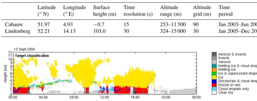
The vertically pointing Doppler cloud radar and backscat-ter lidar are the most relevant instruments for the Cloudnet target classification (Hogan and O’Connor, 2004). The radar can detect rain, drizzle drops, ice particles, and insects, be-cause it is sensitive to large particles. Cloud droplets and aerosols can be identified from lidar measurements, because the lidar is sensitive to small particles (Illingworth et al., 2007). In the target classification product, each radar/lidar backscatter pixel is classified as liquid droplets, ice, insects, aerosols, clear-sky, or other categories. The target classifica-tion product also contains cloud top height and cloud base height. Cloud top and cloud base heights correspond to the highest and lowest of backscatter altitude grid boxes, respec-tively, that have clouds. Therefore, for multilayer clouds, the cloud top height refers to the top of the highest layer of the clouds and the cloud base height refers to the base of the lowest cloud layer. An example of the Cloudnet target classi-fication product at Lindenberg (Germany) is shown in Fig. 1. At Cabauw (the Netherlands) the target classification prod-uct is produced every 15 s at 90 m vertical resolution. At
Lindenberg, the cloud profile has a time resolution of 30 s and a vertical resolution of 30 m. A summary of the Cloud-net target classification product at Cabauw and Lindenberg is given in Table 1.
2.4 Simulated FRESCO retrievals for SCIAMACHY In order to understand the validation results shown later on, O2A band spectra of several cloud cases are simulated using the Doubling-Adding KNMI (Royal Netherlands Meteoro-logical Institute) code (DAK) and retrievals are performed using the FRESCO algorithm. DAK is a plane-parallel radia-tive transfer model with pseudo-spherical correction at large solar zenith angles (De Haan et al., 1987; Stammes, 2001). It includes multiple scattering and polarization. The clouds can be specified at any layer of the atmosphere and differ-ent scattering phase matrices for clouds can be used. The gas absorptions are calculated line-by-line using the parameters from the HITRAN 2008 database (Rothman et al., 2009). In the simulations, the clouds are at 5 different heights: (a) cloud top at 2 km and cloud base at 1 km, (b) cloud top at 6 km and cloud base at 5 km, (c) cloud top at 10 km and cloud base at 9 km, (d) cloud top at 6 km and cloud base at 2 km, and (e) cloud top at 10 km and cloud base at 3 km, respectively, to represent low, middle, high clouds, thick middle clouds, and thick high clouds. The COT values are 5, 15, and 35 for cloud cases a–c and 15, 35, and 60 for cloud cases d and e. The scat-tering phase matrix for water clouds is calculated using Mie theory. The cloud droplets have a two-parameter gamma size distribution with an effective radius of 6 µm and an effective variance of 0.15 µm. Surface albedos (As) of 0.05 and 0.3 are used to represent the albedo of ocean surface (dark surface) and grass-covered surface (bright surface) at 758 nm, respec-tively. The O2A band spectra are simulated at 0.01 nm res-olution and convolved with the spectral response function of SCIAMACHY (full width at half maximum about 0.45 nm). Ten solar zenith angles and 10 viewing zenith angles between 0 and 85◦ are used in the simulations. We use the midlati-tude summer atmospheric profile (Anderson, 1986) and the surface height is assumed to be 0 km. The geometric cloud fraction is 1. Simulations have been performed before to un-derstand the FRESCO retrievals (Wang et al., 2008; Sneep et al., 2008), but those simulations were only representative for clouds over a dark surface. Because the Cabauw and Lin-denberg Cloudnet sites are both covered with vegetation, the new simulations should provide a better physical explanation of the validation results.
Table 1. Information on the Cloudnet target classification product at Cabauw and Lindenberg.
Latitude Longitude Surface Time Altitude Altitude Time
(◦N) (◦E) height (m) resolution (s) range (m) grid (m) period
Cabauw 51.97 4.93 −0.7 15 253–11 500 90 Jan 2003–Jun 2005
Lindenberg 52.21 14.13 103.0 30 324–15 000 30 Jan 2005–Dec 2011
Figure 1. Quick-look image of the Cloudnet target classification product at Lindenberg on 13 September 2004 (downloaded from www. cloud-net.org).
bright surface, the light path between the surface and clouds becomes important, while this long light path is missing in the FRESCO cloud model. The retrieval tries to simulate this long light path by reducing the cloud fraction and putting the cloud at a high altitude. In this case, the FRESCO retrievals have larger errors. For optically thick clouds, at COT≥35, the surface albedo has almost no impact on the reflectance at the top of the atmosphere. Consequently, FRESCO-retrieved cloud heights are very similar for the dark and bright sur-faces. The chi-square values are larger for theAs=0.3 cases than for the As=0.05 cases, which suggests that the fit is better over a dark surface.
3 Methodology
The FRESCO and ESA L2 cloud products are processed us-ing the same SCIAMACHY L1 data. The SCIAMACHY FRESCO and ESA L2 global cloud products are first in-tercompared to show the general features of the O2A band cloud retrievals and to give more statistics. Next, the valida-tion is performed using collocated SCIAMACHY data and Cloudnet radar/lidar measurements.
The Cloudnet target classification product and cloud boundaries at Cabauw and Lindenberg are used for the val-idation of SCIAMACHY cloud height products, because they have long continuous data sets: from January 2001 to June 2005 at Cabauw and from January 2005 until now at Lindenberg. For the validation the Cloudnet and SCIAMACHY measurements from January 2003 to Decem-ber 2011 are used to construct a collocated data set.
For every SCIAMACHY pixel covering Cabauw or Lin-denberg, 1 h of Cloudnet target classification data, centered at the SCIAMACHY overpass time (±30 min), is selected as collocated data. Thus, for every cloud height measurement
from SCIAMACHY there are about 240 (temporal)×126 (vertical) radar/lidar backscatter pixels at Cabauw and 120 (temporal)×450 (vertical) radar/lidar backscatter pixels at Lindenberg, which are classified as one of the 10 categories or clear-sky. The categories “ice” and “cloud droplets only” are used to determine ice and water clouds (see Fig. 1). The categories with “drizzle” and “rain” usually occur at the cloud base, so they have no impact on the SCIAMACHY cloud retrievals. The cloud radars at Cabauw and Lindenberg are operated at 35 GHz. Only in heavy rain can the sensitiv-ity of the cloud radars to high clouds be affected (Illingworth et al., 2007). Therefore, the cases with precipitation are in-cluded in the validation data set. The radars can miss some high clouds with optical thickness of less than 0.1. This has no impact on the intercomparison because these thin clouds cannot be observed properly by SCIAMACHY.
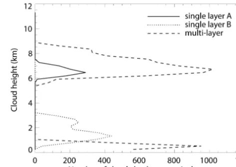
Height distributions of the radar/lidar backscatter pixels are derived for ice clouds, water clouds, and both types, re-spectively, from 250 to 12 000 m with a bin size of 270 m. Some examples of cloud height distributions are shown in Fig. 3. If the distribution has a single mode without inter-ruption by clear-sky pixels, the cloud case is classified as a single-layer cloud. If more than one mode appears in the distribution and these modes are separated by clear-sky pix-els, the case is classified as a multilayer cloud. As illustrated in Fig. 3, single-layer cloud A has a single peak, whereas single-layer cloud B has two local peaks; but since there are no clear-sky pixels between the two peaks, case B is classi-fied as a single-layer cloud.
Figure 2. FRESCO-retrieved cloud heights for simulated cloud cases for a solar zenith angle of 60◦and nadir view. The cloud op-tical thickness values areτ1=5,τ2=15,τ3=35,τ4=60. Cloud top and base heights are indicated using blue horizontal lines. The surface albedos (As) are 0.3 and 0.05.
separated into water and ice clouds. The Cloudnet cloud top height is the arithmetic mean of the cloud top heights in a 1 h period around the SCIAMACHY overpass time; the same holds for the cloud base height. We define a “cloud middle height”, which is the arithmetic mean of the heights of the targets which are classified as “ice” and/or “cloud droplets only”. The cloud middle height depends on the cloud height distribution; it often differs from the mean of cloud top and cloud base heights.
In the validation of FRESCO and ESA L2 cloud heights using the Cloudnet data, we are mainly focusing on the scenes having effective cloud fractions larger than 0.1. This criterion is necessary because the ESA L2 cloud top heights are often not retrieved for scenes having an effective cloud fraction smaller than 0.1. The ESA L2 cloud product pro-vides flags in bits for the quality of the SACURA retrievals, which can be interpreted in the following categories: (1) full convergence, (2) number of iterations exceeded, (3) cloud layer size set to constraint, (4) cloud bottom height set to constraint, (5) cloud top height set to constraint, and (6) no convergence. If the algorithm does not converge, the cloud top height is a filled value (−99.9). If the ESA L2 cloud frac-tion is 0, cloud top height is also 0. For the retrievals having flags of 1–5, the cloud top heights are provided in a range of 1–17 km. The full convergence retrievals have an error of 0.25 km for cloud top height, while the retrievals with con-straints have an error of 0.5 km (Meringer, 2010). Because we would like to evaluate the quality of the complete cloud top height product, we use all the ESA L2 cloud top heights between 1 and 17 km which means the data having flags 1–5 are used.
Figure 3. Three examples of Cloudnet cloud vertical distributions: two single-layer cases and one multilayer case. The distributions are based on 1 h of data centered at the SCIAMACHY overpass time (about 10:00 LT).
4 Results
4.1 Global intercomparison of FRESCO and ESA L2 cloud products
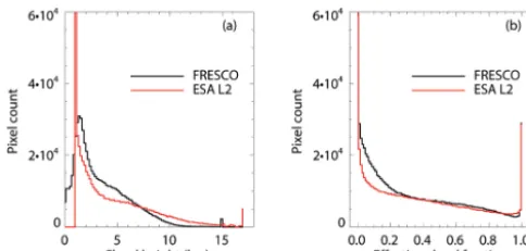
Figure 4. (a) Histogram of SCIAMACHY FRESCO cloud height and ESA L2 cloud top height for global data. (b) Histogram of SCIAMACHY FRESCO effective cloud fraction and ESA L2 cloud fraction. The pixel count for the ESA L2 product (out of range in the plots) is 1.6×10⁵at cloud height of 1 km in (a) and is 2.0×10⁵ at effective cloud fraction of 0.0 in (b).
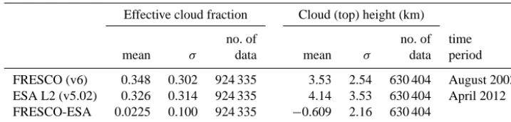
SCIAMACHY L1 measurements has no obvious effect on neither the cloud fraction nor the cloud (top) height retrieved by the investigated algorithms. The global statistics of the FRESCO and ESA L2 cloud products are summarized in Ta-ble 2.
The global frequency distributions of the FRESCO cloud height and ESA L2 cloud top height are shown in Fig. 4a. Both histograms have a maximum at 1–2 km, which indi-cates the global dominance of low clouds. The ESA L2 cloud top height distribution is cut off at 1 km as the low-est value, which is a feature of the SACURA algorithm. The FRESCO mean cloud height is 0.6 km lower than the ESA L2 mean cloud top height. The difference between ESA L2 and FRESCO cloud heights decreases with increasing ESA L2 COT because both FRESCO and ESA L2 cloud algorithms are most suitable for optically thick clouds (see Sect. 2). The difference between ESA L2 and FRESCO cloud heights does not depend on the effective cloud frac-tion, the solar zenith angle or the ESA L2 convergence flags. These differences can be understood from the principles of the FRESCO and SACURA algorithms. Both algorithms re-trieve the cloud height from the amount of O2absorption at 760 nm, which determines the length of the light path above the cloud and inside the cloud. Multiple scattering inside the cloud is taken into account in the SACURA algorithm but not in the FRESCO algorithm. In FRESCO the light path of photons inside the cloud is added to the light path above the cloud. Therefore, FRESCO retrieves a lower cloud height than SACURA. As shown in Fig. 2, FRESCO effectively re-trieves a cloud midlevel height, especially over dark surfaces. The FRESCO-retrieved cloud height increases with increas-ing COT for geometrically thick clouds. This may explain the COT dependence of the difference between the ESA L2 and FRESCO cloud heights. In reality, the retrieved cloud heights could be different from the simulations due to differ-ent cloud optical properties and differdiffer-ent solar and viewing geometries.
The FRESCO effective cloud fraction and the ESA L2 cloud fraction, shown in Fig. 4b, have similar distributions except at effective cloud fractions of less than 0.2. In that range the ESA L2 cloud fraction product is sharper peaked (more cloud-free pixels), whereas the FRESCO effective cloud fraction product has a wider distribution. Because the cloud fraction in the ESA L2 product is derived from PMDs, which have a pixel size of about 7 km×30 km, it has slightly more clear-sky pixels than FRESCO (Krijger et al., 2007). This may cause differences between ESA L2 cloud fraction and FRESCO effective cloud fraction at small cloud frac-tions. However, the ESA L2 cloud fraction and FRESCO ef-fective cloud fraction are very similar: the global mean dif-ference (ESA L2 – FRESCO) is only−0.023 (6 %) with a standard deviation of 0.1. The consistence between the ESA L2 cloud fraction and FRESCO effective cloud fraction sug-gests that the ESA L2 cloud fraction is actually an effective cloud fraction for optically thick clouds (with cloud albedo of 0.8). The relationship between geometric cloud fraction and effective cloud fraction has been described by Stammes et al. (2008).
4.2 Validation
From January 2003 to December 2011, there are 693 collo-cated SCIAMACHY and Cloudnet measurements, of which 157 cases are excluded because of almost cloud-free con-ditions (Cloudnet cloud fraction<0.05). In the remaining 536 cases, 297 cases are single-layer clouds and 239 cases are multilayer clouds. The single-layer cloud cases with FRESCO effective cloud fraction>0.1 (217 cases) include 71 cases of water clouds (class “cloud droplets only”), 103 cases of ice clouds (class “ice”), and 43 cases having co-existing water and ice clouds. For the multilayer clouds, ice and water clouds are not analyzed separately, because most multilayer clouds have both ice and water cloud droplets. The number of cloud-free cases is 99 according to the Cloud-net products. According to the ESA L2 product there are 82 cloud-free cases. This difference can occur due to errors in the satellite cloud detection technique, and due to partial col-location, e.g., if the Cloudnet site is located at the edge of the SCIAMACHY pixel. For the cloud-free pixels in the ESA L2 cloud product, the mean of the FRESCO effective cloud frac-tions is 0.0244. This is in good agreement with the global dif-ference of 0.0225 between the FRESCO and ESA L2 cloud fractions (see Table 2).
4.2.1 Single-layer clouds
Table 2. Statistics of SCIAMACHY FRESCO (v6) and ESA L2 (v5.02) global cloud products,σ– standard deviation.
Effective cloud fraction Cloud (top) height (km)
no. of no. of time
mean σ data mean σ data period
FRESCO (v6) 0.348 0.302 924 335 3.53 2.54 630 404 August 2002–
ESA L2 (v5.02) 0.326 0.314 924 335 4.14 3.53 630 404 April 2012
FRESCO-ESA 0.0225 0.100 924 335 −0.609 2.16 630 404
Figure 5. Scatter plots of SCIAMACHY FRESCO cloud height vs. Cloudnet cloud top height, for (a) all layer clouds, (b) single-layer water clouds, and (c) single-single-layer ice clouds. The color of the symbol indicates the FRESCO effective cloud fraction, with the color code given by the vertical bar. The black line is the one-to-one line. For the points with c_fresco>0.1, the correlation coefficients are (a) 0.685, (b) 0.206, and (c) 0.489.
because some single-layer clouds have both ice and water droplets. If the FRESCO effective cloud fraction is less than 0.1, the FRESCO cloud heights show large scatter. FRESCO cloud heights are in good agreement with Cloudnet cloud top heights for low clouds, but are lower than the Cloud-net cloud top heights for high clouds. This behavior does not depend on the effective cloud fraction. The linear cor-relation coefficients andpvalues are calculated for the data in Fig. 5 for the cases having effective cloud fraction>0.1. The correlation coefficients are tested for their significance and expressed as ap value. A smallp value suggests that the correlation is significant. Results having apvalue<0.01 are defined significant in this paper. The criteria on effective cloud fraction andpvalue are also applicable to all correla-tion analyses in Sect. 4. The correlacorrela-tion coefficients between the FRESCO cloud height and the Cloudnet cloud top height are 0.685, 0.206, and 0.489 for all, water, and ice (single-layer) clouds, respectively. The correspondingp values for all, water, and ice clouds are 0.0, 0.170, and 1.75×10⁻⁵. According to the above definedp value threshold, the lin-ear correlation between the FRESCO cloud height and the Cloudnet cloud top height is significant for all clouds and ice clouds, but not for water clouds. The small correlation coef-ficient for water cloud cases is mainly caused by a few out-liers. The small effective cloud fraction values indicate that these water clouds are optically thin, which is not a favorable condition for the FRESCO algorithm. The correlation coeffi-cient between the FRESCO cloud height and Cloudnet cloud top height is much larger for the cases having large effective cloud fractions.
Figure 6. Scatter plots of SCIAMACHY ESA L2 cloud top height versus Cloudnet cloud top height for (a) all single-layer clouds, (b) single-layer water clouds, and (c) single-layer ice clouds. The color of the symbol indicates the ESA L2 cloud fraction, with the color code given by the vertical bar. The black line is the one-to-one line. For the points with c_lv2>0.1, the correlation coefficients are (a) 0.451, (b) 0.247, and (c) 0.426.
the Cloudnet cloud top height for large cloud fractions. In a cloudy scene, the effective cloud fraction is proportional to the cloud albedo, which increases with increasing cloud optical thickness (Stammes et al., 2008). Figure 6 indicates that the difference between the ESA L2 cloud top height and the Cloudnet cloud top height may be related to cloud opti-cal thickness. The correlation coefficients between the ESA L2 cloud top height and the Cloudnet cloud top height are 0.451, 0.247, and 0.426 withpvalues of 4.24×10⁻¹⁰, 0.188, and 1.66×10⁻³for all clouds, water clouds and ice clouds,
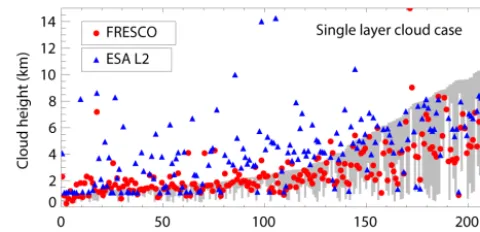
Figure 7. Comparison between SCIAMACHY ESA L2 cloud top height, FRESCO cloud height, and Cloudnet cloud top and cloud base height for single-layer clouds. The cases are sorted according to the Cloudnet cloud top height. The grey bar indicates the altitude range of the cloud according to the Cloudnet product. Here the cases with FRESCO effective cloud fraction below 0.1 are excluded.
respectively. Therefore, the correlation coefficients are sig-nificant for all clouds and ice clouds. In Fig. 6b, the small cor-relation coefficient for water cloud cases is caused by some outliers and by the cases where the ESA L2 cloud top heights are set to constraint at 1.1 km. As shown in Fig. 6b the ESA L2 cloud top height and the Cloudnet cloud top height have a good linear correlation for water clouds having c_lv2>0.7.
Figure 7 shows the single-layer cloud cases sorted accord-ing to the Cloudnet cloud top height. The grey bar marks the Cloudnet cloud vertical range from cloud base height to cloud top height. The red and blue points indicate the FRESCO cloud height and ESA L2 cloud top height, re-spectively. These are the same single-layer cloud cases as in Figs. 5 and 6, but excluding the cases that have a FRESCO ef-fective cloud fraction of less than 0.1. For the cases in Fig. 7, the mean and median of the geometric cloud fraction derived from the Cloudnet measurements are, respectively, 0.84 and 0.99. Therefore, most of the cases are fully cloudy for 1 h of collocated Cloudnet measurements. The mean variations of Cloudnet cloud top and cloud base heights within an hour are both about 340 m and the medians about 220 m.
amount of O2 absorption in scenes with thin cirrus can be very close to that of cloud-free scenes. Therefore, any small errors in the simulated O2 absorption would cause the re-trieval not to converge or yield a cloud height close to the surface or the upper limit of 15 km.
For the low clouds in Fig. 7, the FRESCO cloud height and ESA L2 cloud top height are often higher than the Cloudnet cloud top height. Furthermore, the ESA L2 cloud top height is very noisy. We have further analyzed these low cloud cases (Cloudnet cloud top height<2 km). In Fig. 7 the cloud cases 0–81 are used in the following analysis. The SZA in these 82 cases is in the range of 31–78◦ with a mean SZA of 55◦. The ESA L2 COT values are from 5 to 101 and include some filled values (−99.9), which is due to low reflectance (COT<5). Although the ESA L2 COT may have a bias or a large error in some cases, the COT for the single-layer clouds are more reliable than for the multilayer clouds (Rozanov and Kokhanovsky, 2004) and are retrieved consistently. For the simulated cloudy cases shown in Fig. 2, the effective cloud fractions over a dark (bright) surface are 0.3 (0.2) for COT of 5. This suggests that the cases having ESA L2 COT of−99.9 may have COT<5 and an effective cloud fraction>0.1.
For the cases where FRESCO cloud heights are higher than the Cloudnet cloud top heights, the median of the ESA L2 COT is 9 with some filled values; the mean and median of the SZA are 63◦and 68◦, respectively. From the simulations in Sect. 2.4 we find that the FRESCO-retrieved cloud height can be above the cloud top over a bright surface if COT is smaller than 15 and for large SZA (>60◦). For the low cloud cases with COT = 5 and As= 0.3, the FRESCO-retrieved cloud height is higher than the cloud top at SZA = 70◦. If
COT is<5, the simulated FRESCO cloud height would be above the cloud top height at slightly smaller SZA. In the 82 cases, the difference between the FRESCO cloud height and the Cloudnet cloud top height tends to increase with increas-ing SZA with a slope of about 0.03 km degree−1. Based on the simulations of Sect. 2.4 we may conclude that for low clouds, the fact that the FRESCO cloud height is higher than the Cloudnet cloud top height, is caused by the bright surface (As= 0.3), small COT, and large SZA.
The difference between the ESA L2 and the Cloudnet cloud top height is larger at small COT and smaller at large COT for these 82 low cloud cases. For 5≤COT<15, 15≤COT<35, and COT≥35, the mean (median) of the cloud top height differences (ESA L2 – Cloudnet) are 2.9 (2.5), 0.9 (0.4), and 0.1 (0.2) km, respectively. For the ESA L2 data, the reason for the positive bias could be attributed to small COT, while it has no correlation with SZA. Because the approximation used in SACURA is more accurate for op-tically thick clouds, it is not a surprise that the retrievals are more accurate at large COT. The bright surface and the cloud phase function might contribute to the bias. Although most low clouds are water clouds, there are mixed-phase clouds. Retrieval errors in SACURA related to a bright surface may need more investigation.
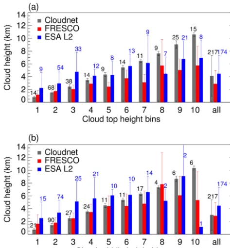
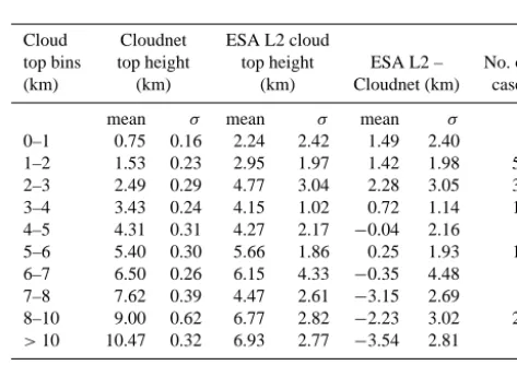
Because the Cloudnet cloud top height covers a range of 0.25–12 km, it would be too coarse to give only a mean dif-ference. SCIAMACHY cloud heights and Cloudnet cloud heights for single-layer clouds have been analyzed for ver-tical bins. The Cloudnet cloud top heights are divided into 1 km bins from 0 to 8 km, a bin for 8–10 km and a bin above 10 km. For every Cloudnet cloud top height bin, the cor-responding FRESCO cloud heights and ESA L2 cloud top heights are selected and the mean and standard deviations are calculated. The results are presented in bar plots in Fig. 8. The number of cases in each bin is the same for the Cloud-net data and FRESCO data, while the number of cases for ESA L2 data is generally less because of non-convergence or no retrievals. Therefore, the number of Cloudnet cloud data in every bin used to compare with ESA L2 cloud top height is less than that used to compare with FRESCO cloud height. For the clarity of the figures, in Figs. 8 and 12, only the Cloudnet cloud heights for collocated FRESCO cloud heights are shown. The Cloudnet cloud heights for collocated ESA L2 cloud top heights are provided in the tables in the Appendix. As shown in Fig. 8a, below 4 km the FRESCO cloud height is close to the Cloudnet cloud top height; the differences are between 0.20 km (bin 2) and−0.57 km (bin 4), which include 62 % of 217 cases. The ESA L2 cloud top height is close to the Cloudnet cloud top height for the bins at 4–7 km; the differences are between−0.04 km (bin 5) and 0.72 km (bin 4), which include 24 % of 174 cases. However, the mean difference between ESA L2 and Cloudnet cloud top heights is small: the ESA L2 cloud top height is only 0.44 km higher than the Cloudnet cloud top height, with a standard deviation of 3.07 km. FRESCO cloud height is about 1.25 km lower than the Cloudnet cloud top height, with a standard de-viation of 2.31 km.
Figure 8b shows the comparisons for 1 km bins of the Cloudnet cloud middle height and the SCIAMACHY cloud height products. The number of data in each bin is different from Fig. 8a, because a Cloudnet cloud can fall into a dif-ferent bin by considering the cloud top height or the cloud middle height. For example, in bin 10 the number of Cloud-net cloud top heights is 15 but the number of CloudCloud-net cloud middle heights is 6. The FRESCO cloud height has a good agreement with the Cloudnet cloud middle height for 85 % of the cases and for the bins from 0 to 6 km. The smallest difference of 0.01 km occurs in the 2–3 km bin. The mean difference between the FRESCO cloud height and the Cloud-net cloud middle height is only−0.14 km, with a standard deviation of 1.88 km. The values that are used in Fig. 8 are provided in Tables A1–A4 in the Appendix.
Figure 8. (a) Bar plot of Cloudnet cloud top height, FRESCO cloud height and ESA L2 cloud top height in 1 km bins of Cloudnet cloud top height, for single-layer clouds. The height ranges of bins 1–10 are 0–1, 1–2, 2–3, 3–4, 4–5, 5–6, 6–7, 7–8, 8–10, and >10 km. The bin “all” is the mean of bins 1–10. The number above the bar indicates the number of cases; the number of cases for FRESCO is the same as for Cloudnet. The error bar indicates the standard deviation of the data. (b) Same as (a) but for the Cloudnet cloud middle height bins.
of the SCIAMACHY cloud heights for different cloud (top) height ranges. If one would use SCIAMACHY cloud data for some regions dominated by low clouds, then according to Tables A1–A4 in the Appendix the FRESCO cloud prod-uct would be a good option. For middle level and high cloud data, the ESA L2 cloud top height may be used. The global comparison of FRESCO cloud height and ESA L2 cloud top height also suggests that SACURA retrieves more middle and high clouds than FRESCO. Depending on different ap-plications, users may prefer cloud top height or cloud height close to the cloud middle. These tables could encourage users to select SCIAMACHY cloud products for their needs.
4.2.2 Multilayer clouds
Both the FRESCO and the SACURA algorithms assume a single-layer cloud in the retrieval model. In case of two-layer cloud systems, the FRESCO cloud height is located between the two cloud layers and closest to the optically thicker layer (Wang et al., 2008, 2012; Sneep et al., 2008). The SACURA algorithm retrieves a cloud top height close to the cloud top of the lower cloud if the high cloud is optically thin. If the
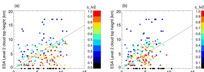
optical thickness of the high cloud layer is larger than 6, SACURA most likely retrieves a cloud top height higher than the top of the high cloud (Lelli et al., 2012). This behavior is also expected in the current comparison. Figure 9 shows the scatter plots of FRESCO cloud height vs. Cloudnet cloud top height and Cloudnet cloud middle height, respectively, for multilayer cloud cases. The FRESCO cloud height is indeed closer to the Cloudnet cloud middle height than to the cloud top height, especially for low multilayer clouds. Similar to the single-layer cloud cases, the FRESCO cloud height can be too high (at 15 km) for clouds with effective cloud frac-tion below 0.1. The correlafrac-tion coefficient between FRESCO cloud height and the Cloudnet cloud top height is 0.509 with ap value of 7.11×10⁻¹⁵. The correlation coefficient be-tween FRESCO cloud height and the Cloudnet cloud middle height is 0.520 and thepvalue is 1.55×10⁻¹⁵. This shows that the correlation between the FRESCO cloud height and the Cloudnet cloud top (middle) height is significant.
The scatter plots of the ESA L2 cloud top height vs. the Cloudnet cloud top height and cloud middle height for multi-layer cloud cases (Fig. 10) show more spread than for single-layer cloud cases (cf. Fig. 6). However, the data points are distributed almost symmetrically along the one-to-one line. The correlation coefficient between the ESA L2 cloud top height and the Cloudnet cloud top (middle) height is 0.330 (0.399) with apvalue of 1.11×10⁻⁵(7.09×10⁻⁸). We can say that the correlation between the ESA L2 cloud top height and the Cloudnet cloud top (middle) height is significant.
The cloud height distributions of multilayer clouds are shown in Fig. 11, as the multilayer analogue of Fig. 7. Here the cases are sorted according to the Cloudnet cloud mid-dle height. The Cloudnet cloud height distribution, indicated by blue-white colors, is normalized to 1 using the maximum occurrence frequency (because of the different temporal and vertical resolutions of the data at Cabauw and Lindenberg, the absolute number of occurrences is different for the two sites). The occurrence frequency can be understood as the relative cloud fraction per altitude bins. The frequency of 1 means fully cloudy. A larger occurrence frequency and a wider distribution indicate more clouds at certain altitudes, which correspond to a large cloud fraction and geometrically thick clouds. As shown in Fig. 11, the FRESCO cloud height agrees well with the peak height of the cloud distribution, up to 5 km. For higher peak heights, the FRESCO cloud height is closer to the lower cloud layers. Most of the FRESCO cloud heights are inside the Cloudnet cloud height distribu-tions. For multilayer clouds Fig. 11 shows that the ESA L2 cloud top height is generally higher than the FRESCO cloud height and lower than the Cloudnet cloud top height, but it does not show a clear relation with the Cloudnet cloud height distribution.
Figure 9. (a) Scatter plot of SCIAMACHY FRESCO cloud height versus Cloudnet cloud top height, for multilayer clouds. (b) Same as (a) but versus Cloudnet cloud middle height. The color of the symbol indicates the FRESCO effective cloud fraction, with the color code given by the vertical bar. The black line is the one-to-one line. For the points with c_fresco>0.1 in (a) the correlation coefficient is 0.509 and in (b) the correlation coefficient is 0.520.
Figure 10. (a) Scatter plot of ESA L2 cloud top height versus Cloudnet cloud top height, for multilayer clouds. (b) Same as (a) but versus Cloudnet cloud middle height. The color of the symbol indicates the ESA L2 cloud fraction, with the color code given by the vertical bar. The black line is the one-to-one line. For the points with c_lv2>0.1 in (a) the correlation coefficient is 0.330 and in (b) the correlation coefficient is 0.399.
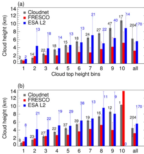
The cloud top heights of multilayer clouds are usually higher than those of single-layer clouds. It appears that the FRESCO cloud height is close to the Cloudnet cloud top height for multilayer low clouds, but we note that only a small percent-age of low clouds are multilayer cloud cases: 19 % for the cloud top height bins and 28 % for cloud middle height bins. Here low clouds refer to clouds in the bins 1–3. The ESA L2 cloud top height for multilayer clouds has about 37 % of cases close to the Cloudnet cloud top height within 1 km. The standard deviation of the differences between the Cloudnet cloud top heights and the ESA L2 cloud top heights is rather large. The statistic results of the comparison between SCIA-MACHY cloud heights and Cloudnet cloud heights for mul-tilayer clouds are given in the Appendix in Tables A5–A8.
Comparing Fig. 12 to Fig. 8, the FRESCO cloud height and ESA L2 cloud top height behave consistently for single-layer and multisingle-layer clouds. However, for the multisingle-layer cloud cases, the differences between SCIAMACHY cloud heights and Cloudnet cloud top and middle heights have larger standard deviations than for single-layer cloud cases.
Multilayer clouds often have an ice cloud layer on top of a water cloud. In this case the ESA L2 COT errors are
rather large (Rozanov and Kokhanovsky, 2004), therefore we do not analyze the cloud height differences as a function of COT. The FRESCO and SACURA algorithms are not de-signed for multilayer clouds; the errors of the SCIAMACHY cloud products can be larger for the multilayer clouds than for the single-layer clouds. Similar to the single-layer cases, Tables A5–A8 in the Appendix may also help the users to choose the proper SCIAMACHY cloud products.
Table 3. Comparison of SCIAMACHY cloud (top) heights with Cloudnet cloud (top) height for selected single-layer clouds. Here, the ESA L2 cloud top height retrievals are fully converged. Cloud fractions derived from the Cloudnet data are 1. The effective cloud fraction is>0.1. “All (c_lv2=1)” has an additional selection criterion of an ESA L2 cloud fraction of 1.
Cloud Cloudnet ESA L2 cloud Cloudnet ESA L2 Cloud
top cloud top top height FRESCO cloud cloud middle optical No. of
bins (km) height (km) (km) height (km) height (km) thickness cases
– mean σ mean σ mean σ mean σ mean σ
1–3 2.18 0.47 5.01 2.4 2.5 1.5 1.58 0.36 15.83 7.35 13
3–6 4.32 1.01 5.16 1.21 2.90 0.8 2.81 0.60 26.86 18.92 13
>6 8.55 1.35 6.86 1.31 4.46 1.17 4.96 0.80 41.73 26.04 18
All 5.42 2.95 5.81 1.87 3.42 1.47 3.32 1.58 29.68 22.45 44
All (c_lv2=1) 8.04 2.44 5.97 1.25 4.15 0.94 4.61 1.20 50.47 17.62 8
Figure 11. Comparison between the SCIAMACHY ESA L2 cloud top height, the FRESCO cloud height, and the Cloudnet cloud height distribution for multilayer clouds. The cases are sorted ac-cording to the Cloudnet cloud middle height. The Cloudnet cloud height distribution is normalized to 1 and indicated with a blue-white color (color code given by the horizontal bar). Here the cases with FRESCO effective cloud fraction below 0.1 are excluded.
4.2.3 Selected cloud cases
The above evaluations have used all the FRESCO cloud heights and ESA L2 cloud top heights provided in the cor-responding products. According to the cloud flag in the ESA L2 data, the fully converged cases should have the smallest error. The FRESCO and SACURA algorithms are more ac-curate for optically thick clouds. Therefore we applied more strict selection criteria in the comparison; namely, single-layer clouds, fully cloudy during 1 h at SCIAMACHY over-pass time at the collocated Cloudnet site (geometric cloud fraction of 1), fully converged in SACURA retrievals and ef-fective cloud fractions>0.1. Using these selection criteria for Cloudnet, FRESCO and ESA L2 cloud products, there are 44 collocated cases. The results are shown in Table 3. For the 44 cases, the mean Cloudnet cloud top height is 5.4 km and the Cloudnet cloud middle height is 3.3 km. The mean FRESCO cloud height is 2.0 km lower than the Cloudnet cloud top height and 0.1 km higher than the Cloudnet cloud
middle height. The mean ESA L2 cloud top height is 0.4 km higher than the Cloudnet cloud top height and 2.5 km higher than the Cloudnet cloud middle height. The mean ESA L2 cloud optical thickness is 29.7 with a standard deviation of 22.5. The mean FRESCO effective cloud fraction is 0.7 with a standard deviation of 0.2. The COT and effective cloud fraction values both suggest that these 44 cases are mainly optically thick clouds. These results are consistent with the comparisons for the single-layer cloud cases in Sect. 4.2.1, where the difference between ESA L2 cloud top height and Cloudnet cloud top height is 0.4 km (see Table A2 in the Ap-pendix) and the difference between FRESCO cloud height and Cloudnet cloud middle height is−0.1 km (see Table A3 in the Appendix).
In the 44 cases, there are 8 cases having an ESA L2 cloud fraction of 1. The comparison for these 8 cases is pre-sented in Table 3 as “All (c_lv2=1)”. These cases are in-cluded in Figs. 5 and 6 for c_lv2=1 and c_fresco=1, re-spectively. Most of these cases are optically and geometri-cally thick ice clouds; their mean cloud top height is 8 km, whereas the water clouds are below 4 km (see Figs. 5b and 6b). The FRESCO cloud height is still close to the Cloud-net cloud middle height and the ESA L2 cloud top height is close to the Cloudnet cloud top height, although slightly lower. SACURA retrieves cloud top height more accurately for single-layer, optically thick water clouds (see Fig. 6b, c_lv2=1 cases). For the ice clouds, the SACURA algorithm may retrieve a lower cloud top height due to the assumptions on the cloud scattering phase function and the cloud water content.
5 Conclusions
Figure 12. (a) Bar plot of Cloudnet cloud top height, FRESCO cloud height and ESA L2 cloud top height in 1 km bins of Cloudnet cloud top height, for multilayer clouds. The height ranges of bins 1– 10 are 0–1, 1–2, 2–3, 3–4, 4–5, 5–6, 6–7, 7–8, 8–10, and>10 km. The bin “all” is the mean of bins 1–10. The number above the bar indicates the number of cases; the number of cases for FRESCO is the same as for Cloudnet. The error bar indicates the standard devi-ation of the data. (b) Same as (a) but for the Cloudnet cloud middle height bins.
is 0.02 smaller than the FRESCO effective cloud fraction with a standard deviation of 0.1. The SCIAMACHY ESA L2 cloud top height is about 0.6 km higher than the FRESCO cloud height with a standard deviation of 2.2 km. The dif-ference between the FRESCO cloud height and the ESA L2 cloud top height is smaller for optically thick clouds and larger for optically thin clouds. This also depends on the ge-ometric thickness. Simulations of FRESCO cloud height re-trievals are performed for different cloud heights and optical thicknesses to interpret the validation results for the SCIA-MACHY FRESCO cloud height. The SCIASCIA-MACHY cloud products are stable over time, which suggests that the SCIA-MACHY L1 7.04 data have a good degradation correction.
The SCIAMACHY cloud height products have been vali-dated using the Cloudnet radar/lidar classification and cloud boundaries at Cabauw and Lindenberg, from January 2003 to December 2011. The collocated cases are separated into single-layer clouds and multilayer clouds according to the height distribution of the radar/lidar backscatter signals dur-ing 1 h (±30 min) around the SCIAMACHY overpass time. In total we found 693 collocated cases. After excluding the
cases with (effective) cloud fractions smaller than 0.1, 421 cases remain; of which 217 cases are single-layer clouds and 204 cases are multilayer clouds.
For single-layer clouds, the difference between FRESCO cloud height and Cloudnet cloud top height is−1.3 km with a standard deviation of 2.3 km; the difference between ESA L2 cloud top height and Cloudnet cloud top height is 0.4 km with a standard deviation of 3.1 km. For single-layer clouds, the difference between FRESCO cloud height and Cloudnet cloud middle height is−0.1 km with a standard deviation of 1.9 km; the difference between ESA L2 cloud top height and Cloudnet cloud middle height is 1.7 km with a standard de-viation of 2.7 km. The evaluation of the ESA L2 fully con-verged single-layer cases shows consistent results with those mentioned above.
The FRESCO cloud height is close to the Cloudnet cloud middle height for both single-layer and multilayer clouds. FRESCO uses a Lambertian cloud model in the forward model and in the retrievals, therefore the light path used in FRESCO is shorter than the real light path in scattering clouds. In order to compensate, the FRESCO-retrieved cloud height is lower than the real cloud top height. For cases with a relatively bright surface albedo, there are too many scat-terings and reflections between the cloud and the surface, for which light path is not included in FRESCO. Therefore, the FRESCO-retrieved cloud height has more scatter over a bright surface than over a dark surface, especially for opti-cally thin clouds.
The ESA L2 cloud top height appears to be close to the Cloudnet cloud top height for middle level clouds, higher than the Cloudnet cloud top height for low clouds, and lower than the Cloudnet cloud top height for high clouds. For the single-layer low clouds, based on the ESA L2 cloud optical thickness, the ESA L2 cloud top height has a larger error for optically thin clouds than for optically thick clouds. Due to its principle, the SACURA algorithm is more suitable for optically thick clouds. The accuracy of the SACURA algo-rithm depends on the accuracy of the geometric cloud frac-tion; therefore the accuracy of the input cloud fraction for SACURA may require further evaluation.
The validation data are analyzed for single-layer clouds and multilayer clouds for 1 km height bins. We find that the error of the FRESCO cloud height is<1 km for clouds be-low 6 km, whereas the ESA L2 cloud top height has an error of<1 km for clouds at 3–7 km, but it has a large scatter.
Based on other satellite cloud height products, globally, 42 % of all clouds are high clouds and about 42 % of all clouds are single-layer low-level clouds (Stubenrauch et al., 2013). We may conclude that, as a global cloud product, FRESCO cloud height is accurate for low clouds, whereas the ESA L2 cloud top height is more accurate for middle level clouds.
The cloud height distributions at Cabauw and Lindenberg, where the SCIAMACHY cloud height validation has been
Appendix A: Statistical results of comparisons between SCIAMACHY cloud heights and Cloudnet cloud heights for single-layer and multilayer clouds in 1 km cloud bins
Table A1. Comparison of SCIAMACHY FRESCO cloud height with Cloudnet cloud top height for single-layer clouds.
Cloud Cloudnet
top cloud top FRESCO cloud FRESCO – No. of bins (km) height (km) height (km) Cloudnet (km) cases
mean σ mean σ mean σ 0–1 0.79 0.15 1.19 0.67 0.40 0.65 14 1–2 1.54 0.24 1.74 0.98 0.20 1.01 68 2–3 2.46 0.29 2.05 0.65 −0.41 0.70 38 3–4 3.47 0.24 2.90 0.92 −0.57 0.81 14 4–5 4.35 0.31 2.44 0.69 −1.90 0.76 9 5–6 5.45 0.33 3.75 1.28 −1.70 1.39 14 6–7 6.48 0.26 3.12 1.26 −3.36 1.27 11 7–8 7.63 0.35 5.74 4.06 −1.89 4.09 9 8–10 9.03 0.58 5.04 1.72 −3.99 1.96 25 >10 10.60 0.33 5.75 3.01 −4.85 2.99 15
All 4.14 3.17 2.89 2.10 –1.25 2.31 217
Table A2. Comparison of ESA L2 cloud top height with Cloudnet cloud top height for single-layer clouds.
Cloud Cloudnet ESA L2 cloud
top bins top height top height ESA L2 – No. of (km) (km) (km) Cloudnet (km) cases
mean σ mean σ mean σ 0–1 0.75 0.16 2.24 2.42 1.49 2.40 9 1–2 1.53 0.23 2.95 1.97 1.42 1.98 54 2–3 2.49 0.29 4.77 3.04 2.28 3.05 33 3–4 3.43 0.24 4.15 1.02 0.72 1.14 12 4–5 4.31 0.31 4.27 2.17 −0.04 2.16 8 5–6 5.40 0.30 5.66 1.86 0.25 1.93 13 6–7 6.50 0.26 6.15 4.33 −0.35 4.48 9 7–8 7.62 0.39 4.47 2.61 −3.15 2.69 7 8–10 9.00 0.62 6.77 2.82 −2.23 3.02 21 >10 10.47 0.32 6.93 2.77 −3.54 2.81 8
Table A3. Comparison of SCIAMACHY FRESCO cloud height with Cloudnet cloud middle height for single-layer clouds.
Cloud Cloudnet FRESCO FRESCO –
middle middle cloud Cloudnet No. of bins (km) height (km) height (km) (km) cases
mean σ mean σ mean σ 0–1 0.73 0.15 1.64 1.42 0.91 1.37 21 1–2 1.42 0.29 1.81 0.81 0.39 0.77 90 2–3 2.50 0.32 2.51 0.80 0.01 0.79 27 3–4 3.55 0.27 3.47 1.24 −0.09 1.20 24 4–5 4.52 0.32 4.40 1.61 −0.12 1.56 11 5–6 5.37 0.27 4.43 1.86 −0.95 1.88 11 6–7 6.33 0.27 4.78 1.98 −1.55 2.02 17 7–8 7.32 0.25 7.82 4.93 0.49 4.80 4 8–10 8.66 0.43 6.08 2.94 −2.58 3.18 6 >10 10.34 0.33 5.33 4.54 −5.01 4.60 6
All 3.02 2.39 2.89 2.10 –0.14 1.88 217
Table A4. Comparison of SCIAMACHY ESA L2 cloud top height with Cloudnet cloud middle height for single-layer clouds.
Cloud Cloudnet ESA L2 ESA L2 –
middle middle cloud top Cloudnet No. of bins (km) height (km) height (km) (km) cases
mean σ mean σ mean σ 0–1 0.70 0.16 2.53 2.52 1.83 2.50 15 1–2 1.40 0.28 3.38 1.95 1.97 1.87 74 2–3 2.53 0.32 5.14 3.08 2.61 3.13 25 3–4 3.56 0.24 5.61 3.28 2.05 3.19 21 4–5 4.48 0.30 6.07 0.96 1.59 0.87 10 5–6 5.36 0.28 6.16 1.97 0.80 1.96 10 6–7 6.36 0.28 6.60 2.49 0.24 2.56 14 7–8 7.11 0.03 5.23 1.83 −1.89 1.87 2 8–10 8.62 0.70 9.08 11.21 0.46 11.90 2 >10 10.34 – 1.15 – −9.19 – 1
All 2.77 1.97 4.47 2.86 1.71 2.71 174
Table A5. Comparison of SCIAMACHY FRESCO cloud height with Cloudnet cloud top height for multilayer clouds.
Cloud Cloudnet FRESCO FRESCO –
top bins cloud top cloud Cloudnet No. of (km) height (km) height (km) (km) cases
mean σ mean σ mean σ 0–1 0.92 0.07 0.78 0.21 −0.14 0.13 2 1–2 1.47 0.35 1.88 0.77 0.42 0.64 14 2–3 2.50 0.35 2.11 1.02 −0.39 0.97 22 3–4 3.54 0.38 2.05 0.94 −1.50 1.08 18 4–5 4.61 0.23 2.76 1.32 −1.85 1.33 15 5–6 5.54 0.28 2.89 1.25 −2.65 1.28 18 6–7 6.48 0.29 2.79 1.19 −3.68 1.20 24 7–8 7.58 0.31 3.63 1.77 −3.95 1.73 27 8–10 8.91 0.57 4.20 2.28 −4.71 2.43 47 >10 10.80 0.44 5.20 2.74 −5.60 2.57 17
Table A6. Comparison of SCIAMACHY ESA L2 cloud top height with Cloudnet cloud top height for multilayer clouds.
Cloud Cloudnet ESA L2 ESA L2 –
top bins cloud top cloud top Cloudnet No. of (km) height (km) height (km) (km) cases
mean σ mean σ mean σ 0–1 0.92 0.07 1.13 0.03 0.21 0.11 2 1–2 1.44 0.34 4.42 3.62 2.99 3.53 13 2–3 2.49 0.36 3.81 3.20 1.32 3.26 18 3–4 3.52 0.39 3.83 2.18 0.32 2.16 14 4–5 4.56 0.27 4.66 2.28 0.10 2.16 13 5–6 5.56 0.26 5.31 2.99 −0.25 3.02 13 6–7 6.43 0.29 7.10 4.66 0.67 4.69 21 7–8 7.59 0.33 5.07 2.95 −2.52 2.96 22 8–10 8.92 0.60 6.39 3.94 −2.52 4.05 40 >10 10.75 0.40 8.88 3.93 −1.87 4.08 14
All 6.21 2.87 5.60 3.76 –0.61 3.91 170
Table A7. Comparison of SCIAMACHY FRESCO cloud height with Cloudnet cloud middle layer height for multilayer clouds.
Cloud Cloudnet FRESCO FRESCO –
middle cloud middle cloud Cloudnet No. of bins (km) height (km) height (km) (km) cases
mean σ mean σ mean σ 0–1 0.81 0.11 1.17 0.56 0.36 0.60 8 1–2 1.58 0.27 1.92 0.58 0.34 0.73 23 2–3 2.42 0.30 2.49 1.23 0.07 1.24 27 3–4 3.57 0.26 2.75 1.03 −0.82 1.01 22 4–5 4.46 0.30 2.82 1.22 −1.65 1.21 37 5–6 5.45 0.31 3.67 1.90 −1.78 1.98 39 6–7 6.41 0.25 4.26 1.88 −2.15 1.86 19 7–8 7.43 0.32 5.28 2.62 −2.14 2.71 16 8–10 8.59 0.49 4.01 1.95 −4.58 2.10 12 >10 10.32 – 13.76 − 3.44 – 1
All 4.50 2.15 3.21 1.96 –1.29 2.02 204
Table A8. Comparison of SCIAMACHY ESA L2 cloud top height with Cloudnet cloud middle height for multilayer clouds.
Cloud Cloudnet ESA L2 ESA L2 –
middle cloud middle cloud top Cloudnet No. of bins (km) height (km) height (km) (km) cases
mean σ mean σ mean σ 0–1 0.81 0.12 2.27 2.48 1.46 2.51 8 1–2 1.58 0.26 4.21 3.48 2.63 3.56 21 2–3 2.45 0.29 4.13 2.18 1.69 2.08 22 3–4 3.58 0.27 5.16 3.00 1.59 2.96 19 4–5 4.44 0.29 5.06 3.09 0.63 3.10 29 5–6 5.46 0.31 6.38 3.83 0.92 3.86 38 6–7 6.40 0.24 6.88 3.66 0.48 3.63 13 7–8 7.37 0.29 9.56 4.12 2.19 4.19 11 8–10 8.68 0.53 8.07 5.47 −0.61 5.64 9 >10 – – – – – – 0
Acknowledgements. We would like to thank our KNMI colleagues Ronald van der A for processing FRESCO data and Henk Klein Baltink and Dave Donovan for help with Cloudnet data. We acknowledge the ESA for the provision of SCIAMACHY L1 and L2 data. We acknowledge the Cloudnet project (European Union contract EVK2-2000-00611) for providing the target classification product, which was produced by the University of Reading and KNMI using measurements from the Cabauw Experimental Site for Atmospheric Research (CESAR), and DWD (German Weather Service) using measurements from the Lindenberg site. This work was supported by the Netherlands Space Office (NSO) as part of the SCIA-Visie project. We are grateful to two anonymous referees and to L. Lelli (Uni-Bremen) for useful comments and suggestions.
Edited by: A. Kokhanovsky
References
Anderson, G. P., Clough, S. A., Kneizys, F. X., Chetwynd, J. H., and Shettle, E. P.: AFGL atmospheric constituent profiles, Tech. Rep. AFGL-TR-86-0110, Air Force Geophys. Lab., Hanscom AFB, MA, 1986.
Boersma, K. F., Eskes, H. J., and Brinksma, E. J.: Error analysis for tropospheric NO2retrieval from space, J. Geophys. Res., 109, D04311, doi:10.1029/2003JD003962, 2004.
Bovensmann, H., Burrows, J. P., Buchwitz, M., Frerick, J., Noel, S., Rozanov, V. V., Chance, K. V., and Goede, A. P. H.: SCIA-MACHY: mission objectives and measurement modes, J. Atmos. Sci., 56, 127–150, 1999.
Bramstedt, K.: Calculation of SCIAMACHY M-Factors, Techni-cal Note, IFE-SCIA-TN-2007-01-CalcMFactor, Issue: 1, avail-able at: http://www.iup.uni-bremen.de/sciamachy/mfactors/ (last access: 10 January 2014), 2008.
Buchwitz, M., Rozanov, V. V., and Burrows, J. P.: A correlatedk distribution scheme for overlapping gases suitable for retrieval of atmospheric constituents from moderate resolution radiance measurements in the visible/near-infrared spectral region, J. Geo-phys. Res., 105, 15247–15262, 2000.
Bucsela, E. J., Celarier, E. A., Wenig, M. O., Gleason, J. F., Veefkind, J. P., Boersma, K. F., and Brinksma, E. J.: Algorithm for NO2vertical column retrieval from the Ozone Monitoring In-strument, IEEE T. Geosci. Remote Sens., 44, 1245–1258, 2006. De Haan, J. F., Bosma, P. B., and Hovenier, J. W.: The adding
method for multiple scattering calculations of polarized light, Astron. Astrophys., 183, 371–391, 1987.
Desmons, M., Ferlay, N., Parol, F., Mcharek, L., and Vanbauce, C.: Improved information about the vertical location and extent of monolayer clouds from POLDER3 measurements in the oxygen A-band, Atmos. Meas. Tech., 6, 2221–2238, doi:10.5194/amt-6-2221-2013, 2013.
Feigelson, E. M. (Ed.): Radiation in a Cloudy Atmosphere, Gidrom-eteoizdat, Leningrad, 280 pp., 1981.
Ferlay, N., Thieuleux, F., Cornet, C., Davis, A. B., Dubuis-son, P., Ducos, F., Parol, F., Riedi, J., and Vanbauce, C.: Toward new inferences about cloud structures from multi-directional measurements in the oxygen A band: middle-of cloud pressure and cloud geometrical thickness from POLDER-3/PARASOL, J. Appl. Meteorol. Clim., 49, 2492– 2507, doi:10.1175/2010JAMC2550.1, 2010.
Hogan, R. J. and O’Connor, E. J.: Facilitating cloud radar
and lidar algorithms: the Cloudnet Instrument
Syn-ergy/Target Categorization product, available at: http:
//www.met.rdg.ac.uk/~swrhgnrj/publications/categorization.pdf (last access: 30 September 2013), 2004.
Illingworth, A. J., Hogan, R. J., O’Connor, E. J., Bouniol, D., Brooks, M. E., Delanoe, J., Donovan, D. P., Eastment, J. D., Gaussiat, N., Goddard, J. W. F., Haeffelin, M., Klein Baltink, H., Krasnov, O. A., Pelon, J., Piriou, J.-M., Protat, A., Russchen-berg, H. W. J., Seifert, A., Tompkins, A. M., van Zadelhoff, G.-J., Vinit, F., Willen, U., Wilson, D. R., and Wrench, C. L.: Cloud-net – continuous evaluation of cloud profiles in seven operational models using ground-based observations, B. Am. Meteorol. Soc., 88, 883–898, 2007.
Joiner, J., Vasilkov, A. P., Bhartia, P. K., Wind, G., Platnick, S., and Menzel, W. P.: Detection of multi-layer and vertically-extended clouds using A-train sensors, Atmos. Meas. Tech., 3, 233–247, doi:10.5194/amt-3-233-2010, 2010.
Joiner, J., Vasilkov, A. P., Gupta, P., Bhartia, P. K., Veefkind, P., Sneep, M., de Haan, J., Polonsky, I., and Spurr, R.: Fast simula-tors for satellite cloud optical centroid pressure retrievals; evalu-ation of OMI cloud retrievals, Atmos. Meas. Tech., 5, 529–545, doi:10.5194/amt-5-529-2012, 2012.
Koelemeijer, R. B. A., Stammes, P., Hovenier, J. W., and de Haan, J. F.: A fast method for retrieval of cloud parameters using oxygen A band measurements from the Global Ozone Monitor-ing Experiment, J. Geophys. Res., 106, 3475–3490, 2001. Kokhanovsky, A. A., Rozanov, V. V., Nauss, T., Reudenbach, C.,
Daniel, J. S., Miller, H. L., and Burrows, J. P.: The semianalytical cloud retrieval algorithm for SCIAMACHY I. The validation, At-mos. Chem. Phys., 6, 1905–1911, doi:10.5194/acp-6-1905-2006, 2006.
Kokhanovsky, A. A., Nauss, T., Schreier, M., von Hoyningen-Huene, W., and Burrows, J. P.: The intercomparison of cloud parameters derived using multiple satellite instruments, IEEE T. Geosci. Remote, 45, 195–200, doi:10.1109/TGRS.2006.885019, 2007.
Krijger, J. M., van Weele, M., Aben, I., and Frey, R.: Technical Note: The effect of sensor resolution on the number of cloud-free observations from space, Atmos. Chem. Phys., 7, 2881–2891, doi:10.5194/acp-7-2881-2007, 2007.
Lelli, L., Kokhanovsky, A. A., Rozanov, V. V., Vountas, M., Sayer, A. M., and Burrows, J. P.: Seven years of global retrieval of cloud properties using space-borne data of GOME, Atmos. Meas. Tech., 5, 1551–1570, doi:10.5194/amt-5-1551-2012, 2012. Lichtenberg, G.: Verification Report OL V 5.0, SCIAMACHY
Level 1b to 2 processing, ENV-VPR-QWG-SCIA-0095, Issue 2, 15 June 2009, available at: http://atmos.caf.dlr.de/sciamachy/ documents/level_1b_2/SCIAVerification_L12_OL5.pdf (last ac-cess: 30 September 2013), 2009.
Lichtenberg, G.: SCIAMACHY Offline Processor Level1b-2 ATBD, Algorithm Theoretical Baseline Document (SGP OL Version 5), 23 March 2011, available at: http://atmos.caf.dlr.de/ sciamachy/documents/level_1b_2/sciaol1b2_atbd_master.pdf (last access: 30 September 2013), 2011.
Loyola, D. G.: Automatic cloud analysis from polar
or-biting satellites using neural network and data fusion
techniques, IEEE T. Geosci. Remote, 4, 2530–2534,
Meringer, M.: ENVISAT SCIAMACHY Level 1b to 2 Off-line processing Input/Output data definition, Doc.No. ENV-ID-DLR-SCI-2200-4, Issue 5/A, Date 19 January 2010, avail-able at: http://atmos.caf.dlr.de/sciamachy/documents/level_1b_ 2/ioddL12ol_5A.pdf (last acess 8 January 2014), 2010. Popp, C., Wang, P., Brunner, D., Stammes, P., Zhou, Y., and
Grzegorski, M.: MERIS albedo climatology for FRESCO+ O2 A-band cloud retrieval, Atmos. Meas. Tech., 4, 463–483, doi:10.5194/amt-4-463-2011, 2011.
Rothman, L. S., Gordon, I. E., Barbe, A., Benner, D. C., Bernath, P. F., Birk, M., Boudon, V., Brown, L. R., Campar-gue, A., Champion, J.-P., Chance, K., Coudert, L. H., Dana, V., Devi, V. M., Fally, S., Flaud, J.-M., Gamache, R. R., Gold-man, A., Jacquemart, D., Kleiner, I., Lacome, N., Lafferty, W. J., Mandin, J.-Y., Massie, S. T., Mikhailenko, S. N., Miller, C. E., Moazzen-Ahmadi, N., Naumenko, O. V., Nikitin, A. V., Or-phal, J., Perevalov, V. I., Perrin, A., Predoi-Cross, A., Rins-land, C. P., Rotger, M., Simeckova, M., Smith, M. A. H., Sung, K., Tashkun, S. A., Tennyson, J., Toth, R. A., Van-daele, A. C., and Vander Auwera, J.: The HITRAN 2008 molec-ular spectroscopic database, J. Quant. Spectrosc. Ra., 110, 533– 572, 2009.
Rozanov, V. V. and Kokhanovsky, A. A.: Semianalytical cloud re-trieval algorithm as applied to the cloud top altitude and the cloud geometrical thickness determination from top-of-atmosphere re-flectance measurements in the oxygen A band, J. Geophys. Res., 109, 5202, doi:10.1029/2003JD004104, 2004.
Rozanov, V. V., Kokhanovsky, A. A., Loyola, D. G., Siddans, R., Latter, B., Stevens, A., and Burrows, J. P.: Intercomparison of cloud top altitudes as derived using GOME and ATSR-2 instru-ments onboard ERS-2, Remote Sens. Environ., 102, 186–193, doi:10.1109/TGRS.2004.825586, 2006.
Sayer, A. M., Poulsen, C. A., Arnold, C., Campmany, E., Dean, S., Ewen, G. B. L., Grainger, R. G., Lawrence, B. N., Siddans, R., Thomas, G. E., and Watts, P. D.: Global retrieval of ATSR cloud parameters and evaluation (GRAPE): dataset assessment, Atmos. Chem. Phys., 11, 3913–3936, doi:10.5194/acp-11-3913-2011, 2011.
Sneep, M., de Haan, J. F., Stammes, P., Wang, P., Vanbauce, C., Joiner, J., Vasilkov, A. P., and Levelt, P. F.: Three-way compar-ison between OMI and PARASOL cloud pressure products, J. Geophys. Res., 113, D15S23, doi:10.1029/2007JD008694, 2008. Stammes, P.: Spectral radiance modeling in the UV-visible range, in: IRS 2000: Current Problems in Atmospheric Radiation, edited by: Smith, W. and Timofeyev, Y., A. Deepak, Hampton, Va., 385–388, 2001.
Stammes, P., Sneep, M., de Haan, J. F., Veefkind, J. P., Wang, P., and Levelt, P. F.: Effective cloud fractions from the Ozone Mon-itoring Instrument: theoretical framework and validation, J. Geo-phys. Res., 113, D16S38, doi:10.1029/2007JD008820, 2008. Stubenrauch, C. J., Rossow, W. B., Kinne, S., Ackerman, S.,
Ce-sana, G., Chepfer, H., Di Girolamo, L., Getzewich, B., Guig-nard, A., Heidinger, A., Maddux, B., Menzel, P., Minnis, P., Pearl, C., Platnick, S., Poulsen, C., Riedi, J., Sun-Mack, S., Walther, A., Winker, D., Zeng, S., and Zhao, G.: Assessment of Global Cloud Datasets from Satellites: Project and Database Ini-tiated by the GEWEX Radiation Panel, B. Am. Meteorol. Soc., 94, 1031–1049, doi:10.1175/BAMS-D-12-00117.1, 2013. Wang, P., Stammes, P., van der A, R., Pinardi, G., and van
Roozen-dael, M.: FRESCO+: an improved O2 A-band cloud retrieval algorithm for tropospheric trace gas retrievals, Atmos. Chem. Phys., 8, 6565–6576, doi:10.5194/acp-8-6565-2008, 2008. Wang, P., Tuinder, O. N. E., Tilstra, L. G., de Graaf, M., and
Stammes, P.: Interpretation of FRESCO cloud retrievals in case of absorbing aerosol events, Atmos. Chem. Phys., 12, 9057– 9077, doi:10.5194/acp-12-9057-2012, 2012.
Wielicki, B. A., Wong, T., Loeb, N., Minnis, P., Priestley, K., and Kande, R.: Changes in Earth’s albedo measured by satellite, Sci-ence, 308, 5723, doi:10.1126/science.1106484, 2005.