Orbiting Carbon Observatory-2 (OCO-2) cloud screening algorithms: validation against collocated MODIS and CALIOP data

www.atmos-meas-tech.net/9/973/2016/ doi:10.5194/amt-9-973-2016

© Author(s) 2016. CC Attribution 3.0 License.

Orbiting Carbon Observatory-2 (OCO-2) cloud screening

algorithms: validation against collocated MODIS and CALIOP data

Thomas E. Taylor1, Christopher W. O’Dell1, Christian Frankenberg2,3, Philip T. Partain1, Heather Q. Cronk1, Andrey Savtchenko4, Robert R. Nelson5, Emily J. Rosenthal5, Albert Y. Chang3, Brenden Fisher3,

Gregory B. Osterman3, Randy H. Pollock3, David Crisp3, Annmarie Eldering3, and Michael R. Gunson3

1_{Cooperative Institute for Research in the Atmosphere, Fort Collins, CO, USA}

2_{California Institute of Technology, Division of Geology and Planetary Sciences, Pasadena, CA, USA} 3_{Jet Propulsion Laboratory, California Institute of Technology, Pasadena, CA, USA}

4_{NASA Goddard Space Flight Center, Code 610.2/ADNET, Greenbelt, MA, USA} 5_{Department of Atmospheric Science, Colorado State Univ., Fort Collins, CO, USA}

Correspondence to: Thomas E. Taylor ([email protected])

Received: 22 October 2015 – Published in Atmos. Meas. Tech. Discuss.: 4 December 2015 Revised: 2 February 2016 – Accepted: 3 February 2016 – Published: 8 March 2016

Abstract. The objective of the National Aeronautics and Space Administration’s (NASA) Orbiting Carbon Observatory-2 (OCO-2) mission is to retrieve the column-averaged carbon dioxide (CO2) dry air mole fraction (XCO2) from satellite measurements of reflected sunlight in the near-infrared. These estimates can be biased by clouds and aerosols, i.e., contamination, within the instrument’s field of view. Screening of the most contaminated soundings min-imizes unnecessary calls to the computationally expensive Level 2 (L2) XCO2 retrieval algorithm. Hence, robust cloud screening methods have been an important focus of the OCO-2 algorithm development team. Two distinct, com-putationally inexpensive cloud screening algorithms have been developed for this application. The A-Band Prepro-cessor (ABP) retrieves the surface pressure using measure-ments in the 0.76 µm O2 A band, neglecting scattering by

clouds and aerosols, which introduce photon path-length dif-ferences that can cause large deviations between the ex-pected and retrieved surface pressure. The Iterative Maxi-mum A Posteriori (IMAP) Differential Optical Absorption Spectroscopy (DOAS) Preprocessor (IDP) retrieves indepen-dent estimates of the CO2and H2O column abundances using

observations taken at 1.61 µm (weak CO2band) and 2.06 µm

(strong CO2band), while neglecting atmospheric scattering.

The CO2and H2O column abundances retrieved in these two

spectral regions differ significantly in the presence of cloud and scattering aerosols. The combination of these two

algo-rithms, which are sensitive to different features in the spectra, provides the basis for cloud screening of the OCO-2 data set. To validate the OCO-2 cloud screening approach, col-located measurements from NASA’s Moderate Resolution Imaging Spectrometer (MODIS), aboard the Aqua platform, were compared to results from the two OCO-2 cloud screen-ing algorithms. With tunscreen-ing of algorithmic threshold param-eters that allows for processing of'20–25 % of all OCO-2 soundings, agreement between the OCO-OCO-2 and MODIS cloud screening methods is found to be '85 % over four 16-day orbit repeat cycles in both the winter (December) and spring (April–May) for OCO-2 nadir-land, glint-land and glint-water observations.

the surface, even when the optical thicknesses are greater than 1.

1 Introduction

NASA’s OCO-2 satellite was launched on 2 July 2014 into a sun-synchronous orbit. After an initial on-orbit satellite bus checkout period, it was inserted into the 705 km Afternoon Constellation, known as the A-Train (L’Ecuyer and Jiang, 2010). From that orbit, it will collect measurements of re-flected solar radiation in tandem with the other A-Train sen-sors such as MODIS-Aqua, CloudSat and Cloud-Aerosol Li-dar with Orthogonal Polarization (CALIOP) (Xiong et al., 2009; Stephens et al., 2002; Winker et al., 2010). The OCO-2 instrument, described in detail in Crisp et al. (2008), contains three co-bore-sighted imaging spectrometers, fed by a com-mon telescope. The light is dispersed via gratings to form two dimensional images of spectra onto a 1024×1024 pixel fo-cal plane array. The three spectral bands, centered at 0.76 µm (O2A band), 1.61 µm (weak CO2band) and 2.06 µm (strong

CO2 band), with resolving powers of 18 000, 21 000 and

21 000, respectively, were chosen to provide high-precision retrievals of XCO2.

The orientation of the satellite bus rotates with latitude to align the optical elements at a constant orientation rela-tive to the principle scattering plane defined by the earth– sun–satellite geometry. With an integration time of 0.33 s, each OCO-2 frame is approximately 2.3 km along-track. The cross-track width of the swath varies from'0.1 km, when the spectrometer slits are oriented along the orbit track, to 10.6 km at nadir, when the spectrometer slits are oriented per-pendicular to the ground track. Cross-track frames are subdi-vided into eight equal footprints, each being approximately 1.3 km wide at nadir. Each footprint contains a single sound-ing comprised of spectra for all three OCO-2 bands. Further details of the instrument and satellite viewing modes can be found in Sects. 2.2 and 2.3 of Bösch et al. (2015).

For scenes containing significant amounts of cloud and/or aerosol, i.e., contamination, the OCO-2 Level 2 (L2) XCO2 retrieval algorithm fails to converge, thus wasting valu-able processing time. More importantly, contamination at even modestly low optical thicknesses (.0.3) can intro-duce scene-dependent biases in the XCO2 (Butz et al., 2011; O’Dell et al., 2012; Guerlet et al., 2013), hindering the abil-ity to accurately determine the sources and sinks on regional scales – the primary objective of OCO-2. It is therefore nec-essary to provide reliable cloud screening on all of the ap-proximately 1 million OCO-2 measurements collected each day. In this work the definition of optical thickness includes the contribution from aerosols, as well as from both ice and water clouds, except where noted. Therefore, for OCO-2, labeling a scene as cloudy indicates the detection of either cloud or aerosol or both.

The OCO-2 sampling approach was designed to mitigate the chances of introducing systematic biases in the retrieved XCO2 values (Bösch et al., 2006, 2011; Crisp et al., 2008). Two primary mitigation strategies related to cloud screening are the satellite’s multiple observation modes and the small native footprint size of the instrument’s field of view (FOV). As discussed in Miller et al. (2007), nadir viewing obser-vations, with the instrument bore sighted directly beneath the satellite orbit track, minimizes the FOV of individual foot-prints. However, nadir viewing yields low signal-to-noise ra-tios (SNRs) over water surfaces, which are very dark in the CO2 channels, making accurate XCO2 retrievals nearly im-possible over much of the globe. Observations in glint view-ing mode, with the bore sight oriented towards the point of specular reflection, maximizes the SNR but yields larger footprint sizes and longer atmospheric optical paths. This increases the likelihood of cloud contamination within the FOV.

The operational viewing strategy of OCO-2 in the early phase of the mission (September 2014 through June 2015) alternated between nadir-only and glint-only observations on successive 16-day ground track repeat cycles. However, on 2 July 2015 (the 1-year launch anniversary) the nominal se-quence was modified to alternate between nadir and glint ob-servations on successive orbits.

The OCO-2 spacecraft can also point the instrument bore-sight at a stationary surface location in the target observation mode, acquiring thousands of observations as it flies over-head. Target sites include validation targets, such as the To-tal Carbon Column Observing Network (TCCON) stations, which return precise XCO2 estimates using direct observa-tions of the solar disk that can be compared to the OCO-2 XCO2 estimates to identify biases (Wunch et al., 2010, 2011). Anywhere from zero to three orbits each day are designated as a target orbit, with acquisition made only when the skies are predicted to be relatively clear and the local target solar zenith angle (SZA) is less than approximately 55◦ (Wunch et al., 2016). However, the current validation study addresses only the global nadir and glint mode data.

Prior to the launch of OCO-2, the algorithm development team had the benefit of working with the Japanese Green-house Gases Observing Satellite (GOSAT) data set (Kuze et al., 2009; Yoshida et al., 2011). Analysis of the A-Band Preprocessor (ABP) cloud screening algorithm performance, similar to that presented here, was published in Taylor et al. (2012). That study concluded that the ABP, alone, yielded agreement with the MODIS cloud screening around 80 % (90 %) of the time over land (ocean) surfaces. The Itera-tive Maximum A-Posteriori Differential Optical Absorption Spectroscopy Preprocessor (IDP) algorithm was not avail-able at that time.

this comparison yields far more collocated samples than the GOSAT comparison reported in (Taylor et al., 2012). The collocation data set for the MODIS comparison is comprised of four 16-day repeat cycles, two in nadir and two in glint viewing, over both a winter (December) and spring (April– May) time range (approximately 50 million soundings in to-tal). For CALIOP, the comparison is performed on the May nadir-land observations. This provides a statistically robust global analysis of the OCO-2 cloud screening performance.

The work presented here is organized as follows. In Sect. 2, the two OCO-2 cloud screening algorithms are de-scribed and their performance on simulated data is sum-marized. Section 3 briefly discusses the OCO-2 B7 data used in this study and introduces the collocated MODIS and CALIOP products. Section 4 provides detailed analy-sis of the cloud screening validation procedure, including optimization of algorithm tuning and the direct comparison against both MODIS and CALIOP. Finally, summary conclu-sions are given in Sect. 5.

2 OCO-2 aerosol and cloud screening algorithms The OCO-2 ABP and the IDP algorithms are applied to the full OCO-2 data set as part of the operational data processing system. Since OCO-2 collects almost 1 million soundings per day, both algorithms are made computationally efficient by neglecting atmospheric scattering by clouds and aerosols in the radiative transfer forward model. ABP does account for Rayleigh scattering by air molecules, which is non-negligible in the O2 A band, while IDP neglects all sources of

scat-tering. By assuming clear-sky conditions, deviations of re-trieved variables from expected values allow for the identi-fication of scenes contaminated by cloud and aerosol. Brief descriptions of both algorithms are given below. In addition, we provide a detailed discussion of the merits of combin-ing the two into a scombin-ingle cloud and aerosol filter and directly compare the performance on a set of simulated radiances.

2.1 The ABP

The ABP algorithm employs Bayesian optimal estimation (Rodgers, 2000) to retrieve surface pressure and surface albedo from high-resolution spectra in the 0.76 µm O2 A

band, which contain a signature due to the absorption of reflected sunlight by oxygen molecules. Using some prior knowledge of the expected values, the retrieved parame-ters can be interpreted to provide information on cloud and aerosol contamination within the FOV of the satellite sensor. The radiative transfer forward model assumes clear-sky conditions (molecular Rayleigh scattering only), such that differences between the modeled and measured radiances are often apparent when the scene contains cloud or aerosol. Es-timates of the surface pressure from this algorithm, differ-enced against values from the nearest 3, 6, 9 or 12 h European Centre for Medium-Range Weather Forecasts (ECMWF)

forecasts, interpolated to the observation, are calculated as 1ps,cld =ps -ps,a. Here, the subscripts refers to the

sur-face, whilea refers to a priori. The value of1ps,cld, along

with the surface albedo (α) and theχ2goodness-of-fit statis-tic are used to identify changes in the expected opstatis-tical path length, allowing scenes to be flagged as cloudy or clear.

The ABP algorithm was introduced and applied to early GOSAT data in Taylor et al. (2012), with further analysis performed on realistic GOSAT simulations given in O’Dell et al. (2012). More detail about this algorithm as applied to OCO-2 can be found in O’Dell et al. (2014). Simulations have demonstrated the ability of the ABP to reliably deter-mine scenes contaminated with mid- or high-altitude clouds, although it sometimes has trouble detecting low level clouds, even when they are optically thick (O’Dell et al., 2012).

2.2 The IDP

The IDP algorithm performs independent, single-band non-scattering retrievals of the CO2and H2O column abundances

using radiances measured in the 1.61 µm (weak) and 2.06 µm (strong) CO2bands. Ratios of the retrieved CO2(RCO2) and H2O (RH2O) column abundances are computed as

Rgas=

VCDW_gas

VCDS_gas, (1)

where VCD represents the vertical column density of the re-trieved gas (CO2or H2O) in the weak and strong absorption

bands.

2.3 Combing ABP and IDP on simulated data

Following the methodology described in O’Dell et al. (2012), the effectiveness of the combined ABP and IDP filters was tested using simulated OCO-2 and GOSAT measurements. These studies document observable differences in the cloud screening results between OCO-2 and GOSAT and quantify the relative reliability of the ABP for identifying high, thin clouds. They also provide predictions of the performance of the combined ABP and IDP algorithms.

A large set of simulations for both OCO-2 and GOSAT was created via the CSU orbit simulator model (O’Brien et al., 2009), which has realistic distributions of clouds, aerosols, surface types and viewing geometries for both mis-sions. The OCO-2 orbit geometry was adopted for both in-struments. The simulation data set consists of 96 orbits span-ning 3 days in both June and December to cover a full range of solar zenith angles and viewing conditions. Soundings with a sub-satellite point over land were set to nadir view-ing geometry, while those over water were set to view the specular glint spot. A temporal sampling rate of 1 Hz was used. Only the instrument model used to convolve the top-of-atmosphere (TOA) reflected radiances differs between the two sets of simulations.

The major differences in the OCO-2 and GOSAT ments are polarization sensitivity, spectral resolution, instru-ment line shape (ILS) and the noise models. Full details on the specific sensors and calibration procedures can be found in Crisp et al. (2008), O’Dell et al. (2011), Day et al. (2011), Rosenberg et al. (2016), Lee et al. (2016) and Bösch et al. (2015) for OCO-2 and Kuze et al. (2009) and Yoshida et al. (2010) for GOSAT.

O’Dell et al. (2012) found that 20–40 % of thick, low wa-ter clouds or aerosol layers with total optical depth (TOD) &1 can be missed by the ABP for GOSAT simulated obser-vations over land. The culprit appears to be a nearly com-plete cancellation of PPL shortening and lengthening, which can occur for certain combinations of cloud top pressure, cloud optical depth, solar zenith angle and the O2A band

sur-face albedo (e.g., see Sect. 2 of Taylor and O’Brien, 2009). This may be related to the “critical albedo” phenomenon de-scribed in Seidel and Popp (2012). In general, these cancella-tion effects can also occur in the weak and strong CO2bands

but are unlikely to occur in all three spectral regions simulta-neously.

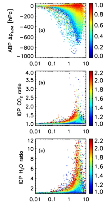
Panel (a) of Fig. 1 shows differences between the surface pressure retrieved by the ABP and the model a priori val-ues,1ps,cld, as a function of the model cloud plus aerosol

optical depth (AOD) for'30 thousand synthetic soundings in nadir viewing mode over land in the month of June. The soundings are colored by the cloud relative height, defined as the height at which the partial-column TOD at 760 nm reaches the smaller of 50 % of the TOD or unity, where the integration begins at the top of the atmosphere. This is a unit-less quantity, as it is normalized by the surface pressure, i.e.,

Figure 1. Scatter plots of (a)1ps,cld, (b) CO2ratio (RCO2) and

(c) H2O ratio (RH2O) versus the total optical depth for OCO-2

sim-ulations over land for the month of June. In panel (a), each sounding is colored according to the cloud relative height (see text), while in panels (b) and (c), each sounding is colored according to the ratio of the 1.6 to the 2.0 µm retrieved effective albedo. The horizontal black lines show the selected threshold values presented in Table 1.

hPa/hPa. Values near 0 (blue colors) represent high cloud or aerosol layers, while values near unity (red colors) represent low cloud or aerosol layers. The horizontal black lines in the figure show thresholds used to separate cloudy scenes from clear sky. The1ps,cldtest is two sided; deviations from the

ECMWF a priori, either high or low, will cause the scenes to be flagged as cloudy.

For the OCO-2 instrument model, the value of1ps,cld

di-verges from 0 at a lower TOD for the high clouds (blue col-ors) than it does for low clouds (red colcol-ors). This is an indi-cator of the ABP’s ability to detect high, optically thin clouds due to strong PPL modification. However, the ABP has more difficulty identifying low clouds, even some that are optically thick, as seen by the large number of bright red data points with small1ps,cldat high TOD. This is due to their relatively

Results (not shown) were quantitatively similar for GOSAT, although the divergence of1ps,cldfrom 0 for high

cloud occurs at higher values of TOD than it does for the OCO-2 instrument model. This suggests a lower sensitivity in the O2A band, implying that the ABP is more sensitive to

contamination by optically thin scattering layers for OCO-2 than for GOSAT. Further tests (not shown) indicate that this is not due to the difference in polarization response between the two instruments. Because their spectral ranges and reso-lutions are similar, the difference could be due to the OCO-2 noise model, which provides higher SNR in the absorption line cores relative to the continuum than does the spectrally uniform noise model of GOSAT. Another explanation for the improved OCO-2 sensitivity to thin clouds may be the much quicker fall off in the ILS wings, which should lead to deeper line cores despite the narrower full width at half maximum of the GOSAT ILS.

The IDP RCO2 andRH2O versus the TOD are shown in panels (b) and (c) of Fig. 1. Here, the color represents the ratio of the 1.61 µm to the 2.06 µm retrieved effective albe-dos,Rα=α1.61 µm/α2.06 µm. In the absence of scattering the

respective RCO2 andRH2O should converge to unity as the light path distributions in the strong and weak bands will be identical, irrespective of differences in surface albedos. For cases with larger TOD, however, the light path distributions will differ between the bands, resulting in ratios that deviate from 1. We found that the ratios almost exclusively deviated in the positive direction, meaning that the PPL in the weak band was larger than in the strong band. This is most likely a consequence of generally lower surface albedos in the strong band as well as higher aerosol sensitivity owing to nearly sat-urated absorption lines.

As the values ofRα diverge from unity (move from blue to red colors in the plots), the IDP RCO2 andRH2O diverge from unity at lower values of the model TOD, thus allowing for more effective screening. In other words, when there are significant differences in the surface albedos of the two CO2

bands, the IDP has higher fidelity in identifying contamina-tion by cloud and aerosol.

Figure 2 compares the fraction of soundings identified as clear by ABP only (blue), IDP only (green) and the combined set (black) for the OCO-2 June nadir-land simulated obser-vations. The total number of scenes and the percent identi-fied as clear are labeled on each panel for the three cloud screening combinations in the corresponding colors. Cloud screening yields are shown for (a) all scenes, (b) high clouds only and (c) low clouds. Here, high (low) cloud is defined as cases where 95 % of the TOD resides in the top 40 % (bottom 30 %) of the atmosphere. About 4 and 18 % of the soundings were classified as high cloud and low cloud cases, respec-tively. The histogram, indicated by the gray shading, shows that there is a large fraction of simulated scenes with optical thickness'3. A similar feature is seen in the real CALIOP data, as will be displayed in Sect. 4.4. The authors currently have no explanation for this seemingly odd feature.

Figure 2. The fraction of simulated OCO-2 soundings identified

as clear by the ABP screen alone (blue), by theRCO2 plusRH2O

(green) and by all three filters combined (black), plotted as a func-tion of the total cloud plus aerosol optical depth (TOD) at 760 nm. The frequency histogram of the TOD is plotted in gray against the right ordinate. Panel (a) shows all cloud cases, while panel (b) shows only those scenes where 95 % of the OD resides in the upper 40 % of the atmosphere (i.e., high clouds) and panel (c) shows cases where 95 % of the OD resides in the lowest 30 % of the atmosphere (i.e., low clouds layers). Only the June nadir-land data are shown.

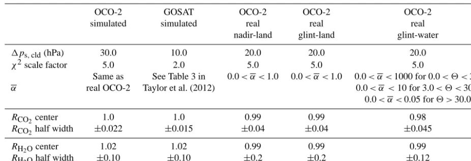
The values of the selected screening variables are provided in Table 1. Details of the ABP1ps,cld,χ2 andα

parame-ters can be found in Sect. III.C. of Taylor et al. (2012). In summary,1ps,cld detects changes in the retrieved versus a

priori surface pressure brought about by scattering-induced PPL modification. The multiplicativeχ2scale factor allows the dynamically calculatedχ2threshold to be scaled. Setting this parameter near unity indicates high confidence in the in-strument calibration and spectroscopy, while very large val-ues (say 20 or greater) effectively disable this test. Moderate values, like those used in this study, cause highly contami-nated soundings to be screened but put most of the burden on the surface pressure check. The third ABP filter is a compari-son of the retrieved surface albedo, averaged over the spectral band end points (α), against predefined lower and upper sur-face albedo thresholds. For all viewing configurations (nadir-land, glint-(nadir-land, glint-water), the lower threshold is set to 0, while the upper threshold is set to unity for land surfaces and varies piecewise as a function of the glint angle for water surfaces. The glint angle,2, is calculated directly from the solar and satellite observation geometries and indicates the angular difference between the sounding center point and the point of solar specular reflection.

Table 1. Settings of the ABP and IDP cloud screening thresholds used for the OCO-2 and GOSAT simulated data sets discussed in Sect. 2.3

and the real OCO-2 data used in Sect. 4.2. Here,2represents the glint angle, as defined in the text.

OCO-2 GOSAT OCO-2 OCO-2 OCO-2

simulated simulated real real real

nadir-land glint-land glint-water

1ps,cld(hPa) 30.0 10.0 20.0 20.0 20.0

χ2scale factor 5.0 2.0 5.0 5.0 5.0

α

Same as See Table 3 in 0.0< α <1.0 0.0< α <1.0 0.0< α <1000 for 0.0< 2 <3.0 real OCO-2 Taylor et al. (2012) 0.0< α <10 for 3.0< 2 <30.0

0.0< α <0.05 for2 >30.0

RCO2center 1.0 1.0 0.99 0.99 0.98

RCO2half width ±0.022 ±0.015 ±0.04 ±0.04 ±0.045

RH2Ocenter 1.02 1.02 0.99 0.99 0.99

RH2Ohalf width ±0.10 ±0.10 ±0.2 ±0.2 ±0.12

RCO2andRH2Othat fall outside the allowed range are flagged as cloudy.

The top panel indicates general agreement between the two cloud screening algorithms in the all-scenes case. For example, when TOD=0.25 about 50 % of the scenes are identified as clear by both ABP and IDP. The combination of ABP and IDP provides a more aggressive screening than a single filter, as seen by the lower fraction of scenes iden-tified as clear at any given TOD. This indicates that ABP and IDP are not flagging identical soundings and are there-fore complimentary. The curves in the plot indicate that all three cloud screening combinations (ABP-only, IDP-only and ABP+IDP) exhibit a smooth decay toward zero fraction passing with increasing TOD. The exception is a noticeable increase in the fraction identified as clear for TOD'3, i.e., a misidentification of cloudy scenes as clear. As mentioned previously, the histogram (gray shading) indicates that there is a large number of scenes with TOD'3. This feature also appears in the real CALIOP data to be presented in Sect. 4.4. This odd feature in the data set is not currently understood.

Panel (b) of Fig. 2 indicates that at TOD = 0.25, the per-cent identified as clear is 0, 4 and 0 % for the ABP, IDP and combined cloud screens, respectively. This is consistent with previous results (Taylor et al., 2012; O’Dell et al., 2012) that show the ABP filter to be extremely effective at screening high clouds. It also suggests that the IDP algorithm is rea-sonably effective at identifying high clouds.

In contrast, the lower panel of Fig. 2 shows that a large fraction of the optically thick, low clouds are not identified by the ABP and to a lesser extent by the IDP. For example, when TOD=1.0, the clear-sky yields are 83, 64 and 61 % for ABP, IDP and combined cloud screens, respectively. This supports the findings for GOSAT presented in O’Dell et al. (2012) and confirms that ABP alone is unlikely to detect low clouds ob-served by OCO-2. However, combining the two filters yields a reduction of about a third of the number of low-altitude, cloud-contaminated scenes with TOD=1, compared to

us-ing the ABP alone. As shown in O’Dell et al. (2012), the re-maining cloud-contaminated scenes do not exhibit PPL mod-ifications in any band and therefore may yield unbiased XCO2 retrievals.

In summary, combining the ABP and IDP cloud filters in tandem yields a cloud and aerosol screener that is more ef-fective at identifying scenes with both high- and low-altitude scattering material then either algorithm alone. Results from these two preprocessors are used in the sounding selection process for the OCO-2 L2 XCO2 retrieval algorithm.

3 OCO-2, MODIS and CALIOP collocated data sets The A-Train is comprised of six satellites flying in tight for-mation that provide near-simultaneous observations from 14 sensors (L’Ecuyer and Jiang, 2010). The OCO-2 reference ground track (RGT) is identical to the CloudSat RGT, which is displaced 217.3 km east of the World Reference System (WRS)-2 track and has an Equator crossing time of 13:30 on the ascending node. This ground track was chosen so that, when OCO-2 is in the nadir observation mode, the sur-face footprints of the spectrometers are centered on the same ground track as the CloudSat radar and Cloud-Aerosol Lidar and Infrared Pathfinder Satellite Observations (CALIPSO) li-dar.

Table 2. Summary of OCO-2 B7 data set to which MODIS and CALIOP collocation were performed. Note that each OCO-2 frame contains

eight footprints, i.e., eight soundings.

Index View mode Start date End date NumDays NumOrbits NumFrames

1 Glint 01 Dec 2014 12 Dec 2014 12 153 1.35 million

2 Nadir 13 Dec 2014 28 Dec 2014 16 228 1.86 million

3 Glint 04 Apr 2015 18 Apr 2015 15 198 1.65 million

4 Nadir 11 May 2015 21 May 2015 11 147 1.13 million

A variety of MODIS-Aqua and CALIOP products, sub-setted to the OCO-2 ground tracks, are being produced by the Cooperative Institute for Research in the Atmo-sphere (CIRA) Data Processing Center (DPC) at Colorado State University in collaboration with the A-Train Data De-pot (ATDD) at the Goddard Earth Sciences Data and In-formation Services Center (GES-DISC). These products are being used for a variety of tasks such as spectral vicar-ious calibration of the instrument and detailed cloud and aerosol analysis. They will be made available to researchers upon request. The work presented here uses these collocated MODIS-Aqua and CALIOP products to provide validation of the OCO-2 cloud and aerosol screening for four sets of 16-day orbit repeat cycles in both nadir and glint viewing modes, as summarized in Table 2.

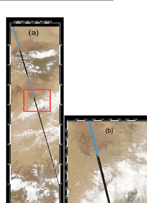
Figure 3 provides an example of the collocation of MODIS pixels to OCO-2 footprints. The OCO-2 spacecraft, and hence spectrometer slit, rotates as a function of latitude, pro-ducing frames that are nearly perpendicular (parallel) to the direction of motion near the equator (poles). Panel (a) pro-vides spatial context of the narrow ('10 km) swath of OCO-2 relative to part of the very wide ('2330 km) MODIS swath. This particular scene is across the Libyan desert in northern Africa on 13 August 2015 (orbit 5930), at which latitudes the OCO-2 slit is aligned non-perpendicular to the motion of the spacecraft, providing a swath width somewhat reduced from the 10 km maximum near the Equator. Panel (b) zooms in on a portion of panel (a) to show the relative size of the OCO-2 footprints against this typical scene of scattered clouds. In both panels, the individual OCO-2 foot-prints are labeled as cloudy (black) or clear (blue) based on the results from the combined ABP and IDP cloud screening algorithms.

Detailed explanation of the collocation technique is pro-vided in the following section.

An analysis of the full OCO-2 data set spanning 6 September 2014 to 1 August 2015 (orbit numbers 958 to 5762) showed that, on average, slightly more than one third (36 %) of the nadir-land soundings pass the ABP operational cloud flag, i.e., are identified as clear, on a per-orbit basis. For nadir-water, glint-land and glint-water observations, the mean per-granule pass rates are 1.9, 26.9 and 23.0 %, re-spectively. The small yield for nadir-water soundings is pre-dominately due to low signal-to-noise ratios, not just because

Figure 3. Demonstration of the collocation of MODIS to OCO-2

for orbit number 5930 (13 August 2015) in nadir viewing mode over central Africa. Panel (a) shows data spanning 20–29◦N lati-tude and 16.4–18.5◦E longitude (450 frames in'150 s). Panel (b) shows a zoomed-in portion of the granule (the red box in Panel (a)) to reveal the relative width of an OCO-2 frame, which is comprised of eight cross-track footprints, each approximately 2 km by 2 km, in relation to a typical scattered cloud deck observed by MODIS. The pixels are colored black (cloudy) or blue (clear) based on the com-bined ABP and IDP cloud screening algorithm results. The cloudy frames north of the visible cloud deck presumably contain sub-visible clouds or aerosols.

operational B7 data set are identifying approximately 20 % of the 1 million daily soundings as clear. Of those soundings that are passed to the L2 retrieval algorithm, approximately 80 % are sufficiently cloud free to yield XCO2 estimates that converge.

3.1 Collocation methodology

The ATDD generates collocated MODIS L1B and L2 atmo-spheric products for many of the satellites in the A-Train con-stellation using the algorithm described in Savtchenko et al. (2008). The main difference in the creation of the OCO-2 product relative to other A-Train sensors is the preparation of the reference track for ingest into the collocation algorithm. In the case of CloudSat, it is most convenient to use the two-line elements of the spacecraft to compute 15 min of Cloud-Sat ground track for every MODIS 5 min granule. However, the OCO-2 flight modes make this simple approach unattain-able. Instead, the geolocation and time information of the central OCO-2 footprint must be extracted from an OCO-2 L1B science granule. Based on that time, an “OpenSearch” request is formulated and sent to the MODIS Processing Sys-tem (LAADS). Upon acquiring the corresponding MODIS 5 min granules (typically nine per OCO-2 granule), a work order is logged with the GES-DISC to push MODIS gran-ules through the processing system. In most cases, part of the processing involves extrapolation of the OCO-2 track us-ing the great arc model. The extrapolation is sufficiently ac-curate to extend the ground track of the OCO-2 footprint so that the resulting reference ground track fully transects the acquired MODIS granules. The resulting output are MODIS-like 5 min HDF-EOS files that contain all the MODIS geolo-cation and science data for a given product within±50 km of the OCO-2 ground target.

Supplemental collocation of the OCO-2 soundings is per-formed at the DPC for MODIS L1A 1 km satellite and scene information, L1B half-kilometer radiances, 1 and 5 km cloud properties, the 10 km aerosol product as well as the CALIOP 1 km cloud layer product and the 5 km cloud and aerosol lay-ered products. As is done at the ATDD, the date and time information is extracted from the OCO-2 L1B files to de-termine the corresponding MODIS and CALIOP granules. Then any product-specific preprocessing is performed and a pixel-by-pixel matching to the OCO-2 geolocation is done. Note that, in the case of MODIS products, the information from all 5 min granules corresponding to a given OCO-2 granule is output to a single file, such that there is a one-to-one file correspondence between the original OCO-2 granule and the collocated MODIS products.

The resultant DPC output HDF-5 files contain geolocation and science data within±50 km of the OCO-2 ground target for MODIS and all geolocation and data for CALIOP. They also contain the geolocation and time information for OCO-2 along with thex andyMODIS or CALIOP pixel location for each match-up, as well as information that allows users

to trace back to the original MODIS and OCO-2 files includ-ing file names, subset start pixel index and collection label. This configuration allows user customization of the match-up process, such as distance-dependent pixel searching.

3.2 MODIS cloud mask

In this work, we define a hybrid MODIS cloud mask by com-bining the standard cloud mask (Ackerman et al., 1998; Frey et al., 2008) with the 1.38 µm cirrus reflectance value (Gao et al., 2002), both contained in the MYD06 cloud product. This follows the procedure first described in Taylor et al. (2012). Each OCO-2 footprint, i.e., a scene, is assigned a reference state of either clear or cloudy based on the fol-lowing MODIS cloud criteria. First, a subset is formed of all 1 km MODIS pixels with center latitude and longitudes falling within 2 km of the center latitude and longitude of an OCO-2 footprint. All scenes in which all of the MODIS pix-els are labeled as confident or probably clear and with cirrus reflectance,R, less than 0.01, are defined as clear sky. If ei-ther of these conditions are violated, then the reference state of the scene is considered to be cloudy. We limit the analysis to MODIS pixels with viewing zenith angle<30◦to avoid oblique lines of sight which can introduce errors (Maddux et al., 2010). No limit is placed on the SZA.

There is a temporal discrepancy between the overpass time of OCO-2 and MODIS of about 7.5 min, during which the ge-ometrical and optical properties of clouds are subject to small changes and/or drifting in or out of the scene. However, er-rors in the validation procedure are mitigated by enforcing the 2 km radial search ('12.5 km2) when matching MODIS pixels to the OCO-2 footprints. This conservative search re-quirement has the added benefit of mitigating sub-FOV cloud effects, which the ABP has been shown to have difficulty identifying via simulations created using a three dimensional radiative transfer model (Merrelli et al., 2015). The effect was shown to lead to biases of up to several parts per mil-lion in XCO2, dependent on the cloud size, surface albedo and illumination geometry, for tropospheric liquid water clouds.

The search criteria produces about 10 matching MODIS pixels per OCO-2 sounding. Tests were performed to ensure that the agreement between OCO-2 and MODIS cloud flags are not overly sensitive to the choice of the search radius, the cirrus reflectance or the sensor zenith angle.

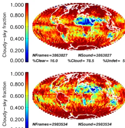
Figure 4. Cloudy-sky fraction calculated from the

MODIS/OCO-2 collocated cloud mask described in Sect. 3.MODIS/OCO-2 for the December combined glint and nadir data sets (top) and the April–May data (bottom). Data are binned in 4◦by 4◦lat/long boxes.

oceans have cloud fractions ranging from about 50 to 100 %. The global mean fraction of cloudy scenes is around 80 %, in close agreement with that reported in Fig. 13 of Miller et al. (2007).

3.3 CALIOP layered data

The CALIOP collocated product used in this work is com-prised of 233 orbits, spanning days 7 to 22 May 2015. For each OCO-2 sounding, the CALIOP data point with the clos-est latitude and longitude to the OCO-2 footprint was se-lected. In this analysis, we limited the data to soundings falling within 5 km to minimize the differences in the ob-served atmospheric and surface conditions. This provided a mean FOV difference of 3.0 km (and about 7 min due to difference in overpass times) for the collection. Two useful cloud metrics, derived from these CALIOP data, were used to analyze the performance of the OCO-2 cloud screening algorithms.

The sum of the cloud and aerosol optical depths at 532 nm, taken from the 5 km cloud and aerosol layered products, respectively, provided the reference total opti-cal depth (TOD532 nm) corresponding to each collocated

OCO-2 sounding. The effective cloud top pressure (pc)

for each CALIOP collocation was calculated by integrat-ing TOD532 nm vertically through the atmosphere (starting

at the top) until TOD532 nm>1 was achieved. The pressure

value at the center of that layer was then assumed to rep-resentpc. This value was then normalized by the ECMWF

model surface pressure (taken from the ABP prior) to give the normalized effective cloud top pressure,p_c. Thus, low-altitude clouds correspond to p_c values near unity, while

clouds higher in the atmosphere are represented byp_c val-ues near 0. This quantity is similar to, but slightly different from, the cloud relative height that was described for the sim-ulations in Sect. 2.3.

Expressions for determiningp_care given as

TOD(pc)=1=

pc

X

p(TOA)

TOD1p, pc=pc/ps, (2)

wherepsgives the surface pressure.

There is a spectral mismatch when comparing the CALIOP measurements at 532 nm, to the OCO-2 cloud screening results, which use measurements taken at 760, 1610 and 2060 nm. It is possible that this could lead to disagreements in classifying contaminated soundings, espe-cially for scenes containing small aerosol particles, i.e., large Ångström coefficients, a condition in which the measure-ments from the two sensors need to be made at the same spectral points. Some errors will exist in the agreement be-tween the two sensors reported in the current study due to this spectral mismatch, as well as the small spatial and temporal discrepancies described above.

4 Validation of OCO-2 cloud screening algorithms 4.1 Contingency table analysis

In this section, we directly compare the OCO-2 and MODIS cloud screening results. This is done via contingency tables (CT), which provide compact summary statistics for compar-ing large predictive data sets. This analysis follows that given in Taylor et al. (2012) on GOSAT data. For each sounding, there are four classification possibilities. The cloud screen-ing algorithms can agree that the scene is clear or cloudy: true positives (TP) and true negatives (TN), respectively. Soundings can also be classified as false positives (FP), when MODIS indicates cloud but OCO-2 identifies the scene as clear, or false negatives (FN), when MODIS indicates clear but OCO-2 cloud. The classification of scenes by MODIS will be referred to as the “reference” state, while scene classi-fication by the OCO-2 preprocessors will be termed the “pre-dicted” state.

Each CT value can be interpreted in terms of a rate, calcu-lated as

true positive rate(TPR) =NTP/Nclear,

false negative rate(FNR) =NFN/Nclear,

false positive rate(FPR) =NFP/Ncloud,

true negative rate(TNR) =NTN/Ncloud,

(3)

whereNTP,NFN,NFPandNTNare the number of collocated

TP, FN, FP and TN soundings, respectively, andNclear and Ncloudgive the number of reference clear and cloudy

Figure 5. Contour plots of the May nadir-land data showing the fraction of soundings passing (top row), agreement (middle row) and positive

predictive value (bottom row) for variations in the ABP1ps,cldversusχ2scale factor (left column), IDPRCO2(middle column) andRH2O

(right column). Contours are drawn at increments of 5 % for the fraction passing and 2 % for the agreement and positive predictive values. The black diamond represents the threshold settings adopted for the analysis presented in this work.

Three useful diagnostic variables can be calculated from the CT values:

throughput=(N_TP+N_FP)/N_total, agreement=(NTP+NTN)/Ntotal,

positive predictive value(PPV)=NTP/(NTP+NFP), (4)

whereNtotal=Nclear+Ncloud=NTP+NFN+NFP+NTNis

the total number of collocated scenes.

The throughput gives the fraction of the total number of collocated scenes that are identified as clear by the OCO-2 cloud screening algorithms. The agreement gives the fraction of scenes that are correctly predicted by the OCO-2 cloud screening algorithms, relative to the MODIS reference state. The positive predictive value (PPV) gives the fraction of the reference clear soundings, i.e., the MODIS clear soundings, also predicted clear by the OCO-2 preprocessors.

4.2 Optimization of the cloud screening algorithm thresholds for the MODIS comparison

We now use CT analysis to explore the optimization of the OCO-2 ABP and IDP cloud screening algorithms by calcu-lating an ensemble of CT diagnostics given in Eq. (4) for varying values of the cloud screening thresholds. This anal-ysis was performed using the OCO-2 data sets that were in-troduced in Sect. 3.

Systematic variations in the threshold values are expected to alter the diagnostic values. The objective is to develop fil-ters such that a tightening (i.e., narrowing) of the thresholds generally yields an increase in the agreement and the PPV, while simultaneously decreasing the throughput. Given fil-ters that satisfy these rules, an aggressive cloud screening can be achieved by tightening the thresholds. Conversely, if the design goal is to filter only the most grossly contaminated scenes while maximizing the throughput at the expense of the agreement, then the filtering thresholds can be set to rela-tively loose values. For OCO-2, our design goal is to pass ap-proximately 25–30 % of soundings without introducing spa-tial sampling biases. This value corresponds to 5–10 % more than the clear-sky fraction observed by MODIS. This infla-tion over the MODIS number is necessary since some of the passed soundings are actually cloudy. It is crucial that as many of the scenes as possible are correctly classified, while limiting the number of false negative cases (MODIS clear, OCO-2 cloudy), as once a sounding has been identified as cloudy by either ABP or IDP, it will not to be run in the op-erational L2 XCO2retrieval algorithm.

The left column of Fig. 5 shows contour plots of the throughput, agreement and PPV for the May nadir-land OCO-2 soundings as a function of the1ps,cld and theχ2

Table 3. Contingency tables for the comparison of the OCO-2 cloud screening preprocessors to MODIS cloud mask. Results are shown for

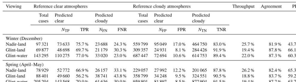
the three main viewing scenarios for both the winter (December) and spring (April–May) data sets.

Viewing Reference clear atmospheres Reference cloudy atmospheres Throughput Agreement PPV Total Predicted Predicted Total Predicted Predicted

cases clear cloudy cases clear cloudy

N_TP TPR N_FN FNR N_FP FPR N_TN TNR Winter (December)

Nadir-land 97 321 73 633 75.7 % 23 688 24.3 % 559 799 95 049 17.0 % 464 750 83.0 % 25.7 % 81.9 % 43.7 % Glint-land 69 877 48 698 69.7 % 21 179 30.3 % 309 357 24 931 8.1 % 284 426 91.9 % 19.4 % 87.8 % 66.1 % Glint-water 143 295 110 275 77.0 % 33 020 23.0 % 687 447 72 694 10.6 % 614 753 89.4 % 22.0 % 87.3 % 60.3 % Spring (April–May)

Nadir-land 78 929 52 772 66.9 % 26 157 33.1 % 229 057 27 992 12.2 % 201 065 87.8 % 26.2 % 82.4 % 65.3 % Glint-land 88 401 49 660 56.2 % 38 741 43.8 % 358 799 34 248 9.5 % 324 551 90.5 % 18.8 % 83.7 % 59.2 % Glint-water 205 204 143 568 70.0 % 61 636 30.0 % 959 801 81 897 8.5 % 877 904 91.5 % 19.4 % 87.7 % 63.7 %

diagnostic parameters simultaneously is evident. In general, as the agreement and PPV increase with tighter choices of 1ps,cld andχ2 scale factor, the throughput decreases. For

this particular data set, setting 1ps,cld to 25 hPa and χ2

scale factor to 5 allows a throughput '42 %, with agree-ment '77 % and PPV '52 %. The operational settings of the OCO-2 ABP since the on-orbit instrument checkout phase (September 2014) have been 25 hPa andχ2scale fac-tor=20. Studies showed that for nadir-land and glint-ocean viewing the 1ps,cld filter alone flags approximately 98 %

of the soundings determined cloudy by ABP, while the sur-face albedo check provides significant filtering (up to 25 % of cloudy scenes) for glint-land viewing.

The inclusive ranges of the IDP RCO2 and RH2O values are described by a center point plus and minus a half-width value. The middle and right columns of Fig. 5 show re-sults from the optimization testing for IDP RCO2 andRH2O half-width versus center point values, respectively. Values of 0.99±0.04 and 0.99±0.2 for nadir-land were selected for RCO2andRH2O, respectively, as shown in Table 1. These val-ues were then implemented in the cloud screen comparison to MODIS that will be detailed in Sect. 4.3. Note that the results for the glint-land and glint-water viewing scenarios differed slightly compared to the nadir-land results, as shown in Ta-ble 1. Furthermore, slight differences were observed between the winter and spring data sets, indicating that the thresholds values should be carefully selected to minimize over-filtering of the data.

4.3 Validation of OCO-2 cloud screening algorithms against MODIS

After optimization of the cloud screening thresholds, contin-gency tables were generated using the combined ABP and IDP algorithms. The analysis was performed separately for each of the three viewing scenarios: nadir-land, glint-land and glint-water using the data sets for the four 16-day repeat cycles referenced in Table 2. The results of the CT analysis are displayed in Table 3.

Overall, the results are very encouraging. The throughputs using the combined ABP and IDP cloud screenings range from 20 % for the spring glint-water data to 31 % for the spring glint-land data. Agreement with MODIS for the six data sets ranges from a low of 79 % for spring glint-land to 88 % for spring glint-water. Finally, the positive predictive values range from 46 % for winter land (both nadir and glint) to 67 % for spring nadir-land.

The roughly 15–20 % of scenes that are in disagreement can be explained by a number of factors, one being the strin-gent MODIS search criteria for defining the reference scene as clear or cloudy. In some cases, one or two of the approxi-mately 10 MODIS pixels that are matched to a single OCO-2 footprint may be labeled as probably or confidently cloudy. This causes the reference scene to be defined as cloudy, al-though the OCO-2 footprint itself may be observing clear-sky. In addition, an OCO-2 footprint can potentially miss sub-FOV clouds as demonstrated by Merrelli et al. (2015). These very same scenes would presumably have been identi-fied as cloudy by MODIS, which has a smaller spatial foot-print. Finally, the OCO-2 “cloud mask” does not discriminate aerosol versus cloud. Therefore, some aerosol-laden clear scenes will be correctly identified by MODIS as clear, and correctly identified by OCO-2 as cloudy, because of this dif-ference in definition.

Another fundamental reason for disagreement between the OCO-2 cloud screening algorithms and MODIS is that the comparisons are in reference to MODIS as truth, an assump-tion that is not void of uncertainties. There are errors inher-ent in comparing cloud screening between satellite sensors with very different instrument characteristics and specifica-tions which are not viewing exactly the same scene with the same viewing geometry at the same time. Furthermore, the cloud screen threshold values were selected to be relatively loose. As was discussed in Sect. 4.2, tighter thresholds gen-erally increase PPV but reduce the throughput.

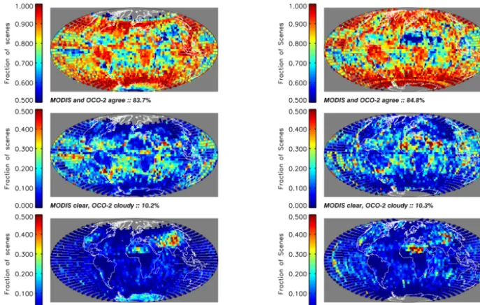
Figure 6. Combined glint and nadir gridded contingency table data for December (left column) and April–May (right column). Data are

binned on a 4◦by 4◦lat/long grid. Scenes for which MODIS and OCO-2 cloud screenings agree are shown in the top panel, while the two types of disagreement – MODIS clear, OCO-2 cloudy and vice versa – are shown in the two lower rows, respectively. The color scales span the range 50–100 % for the “agree” panels and 0–50 % for the “disagree” panels.

(TNR'80–90 %) versus the lower agreement for the refer-ence clear scenes (TPR'65-75 %). This indicates that the OCO-2 cloud screening algorithms, as configured in this study, are more aggressive, i.e., use more stringent filtering thresholds than MODIS does. This makes sense, as OCO-2 is sensitive to both clouds and aerosols, while the MODIS cloud mask product identifies only water and ice clouds.

An investigation of the eight OCO-2 footprints per frame via CT statistics reveals no strong footprint dependence. The range of variability for all of the CT values across footprints is always well under 2 % and is generally closer to 1 %, which is essentially within the noise.

It is critical to avoid latitudinal sampling biases in the mea-surement of XCO2, as these can yield serious errors in flux inversion estimates (Liu et al., 2014). To assess the spatial distributions of the contingency table values in the current analysis, the combined glint and nadir data sets were gridded into 4◦ latitude by 4◦ longitude bins, and the fractions that agree and disagree in each bin were calculated. The results are presented in Fig. 6, which shows the winter data in the left column and the spring data on the right. The top panels show that the global agreement of '85 % in both seasons (and for all viewing geometries) contains large, spatially cor-related regions with>90 % agreement over much of the total land mass as well as the northern Atlantic, northern Pacific, eastern Indian and Southern oceans. Other regions generally have cloud screening agreement '70–80 %, with a few ar-eas agreeing less than 60 % of the time, such as certain ocean regions and northern Africa in April–May.

The middle and bottom panels of Fig. 6 show the two types of disagreement in the cloud screeners: false negatives (MODIS clear, OCO-2 cloudy) and false positives (MODIS cloudy, OCO-2 clear), respectively. The false negative errors tend to occur over tropical and subtropical oceans. The rea-son for this disagreement is unclear, but it seems to imply that these are very thin cloud cases to which OCO-2 is more sensitive than MODIS. The false positive errors, shown in the lower panels, are heavily concentrated over the Sahara and Tibetan plateau land regions, where some grid cells ex-ceed 50 % of scenes in disagreement in spring. These are very likely to be driven by desert dust and topographic features, as discussed below.

collocated product was not available at the time this research was performed. As stated above, the OCO-2 screening al-gorithms do not discriminate between aerosol and cloud, and hence they identify any scenes that are contaminated by cloud and/or aerosol.

The second significant temporal difference feature over land is seen over the Sahara, where the fraction of false positive scenes (MODIS cloudy, OCO-2 clear) increases from about 25 % to more than 50 % from winter to spring. Observations from the Total Ozone Mapping Spectrome-ter (TOMS) indicate increased dust loads over this region during the warmer months (peak in June and July), with a minimum in October and November (Engelstaedter et al., 2006). The reason for the disagreement here is unclear, though it seems unlikely that MODIS would be incorrectly identifying dust-laden scenes as cloudy, while OCO-2 iden-tifies them as clear. These cases warrant further investigation to identify the source of this discrepancy.

Finally, the distribution of the false positive scenes over the Tibetan plateau decreases in spatial extent from winter to spring but becomes more concentrated in the eastern edge. This phenomena may be driven by the extreme topography and/or snow cover of this region, though at this point it is not clear which of the two cloud screeners (MODIS or OCO-2) is in error.

The spatial change in the agree/disagree distribution from winter to spring is less pronounced over ocean compared to land. The most distinct signal is a tracking of the sub-solar point as it moves northward between the seasons. This would indicate a largely SNR-driven issue, i.e., as the SNR of OCO-2 increases, so too does the sensitivity to very mild scatter-ing effects. Most of the disagreements over ocean are of the false negative type (MODIS clear, OCO-2 cloudy), which, as stated previously, could be due to a more sensitive cloud identification by OCO-2 relative to MODIS.

In general, the global patterns in the cloud screening agree-ments between winter and spring look much the same, indi-cating that there does not appear to be strong seasonally de-pendent sampling biases in the OCO-2 cloud screened data set. The spatial and temporal differences have, for the most part, been explained, although a rigorous analysis and verifi-cation of the proposed hypotheses has yet to be made.

4.4 Validation of OCO-2 cloud screening algorithms against CALIPSO

The next step in our validation of the OCO-2 cloud screen-ing algorithms was to assess the cloud screenscreen-ing performance against collocated CALIOP measurements. The CALIOP TOD532 nm and the normalized effective cloud top pressure

(p_c), introduced in Sect. 3.3, were used. CALIOP is more sensitive to low optical thicknesses than MODIS, and it pro-vides information on the vertical structure of scattering lay-ers, allowing for a more quantitative analysis of the OCO-2 cloud screening abilities and a basis for investigating

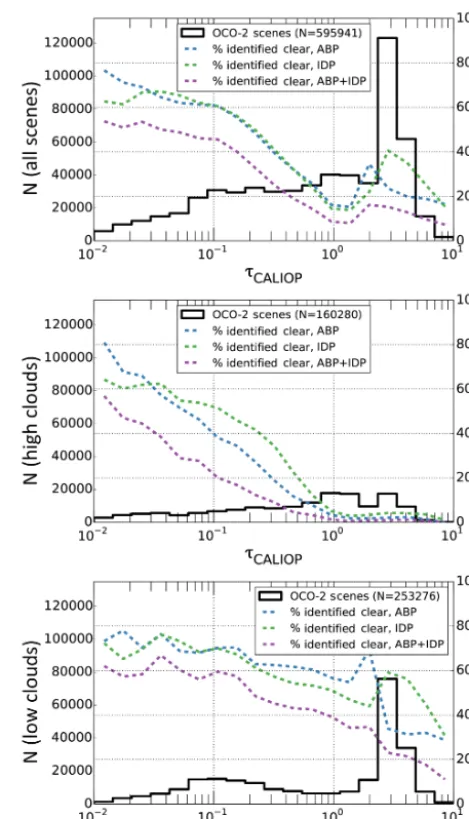
sound-Figure 7. Comparison of OCO-2 cloud screening to CALIOP

opti-cal depth measurements for collocated soundings. Histograms of the number of OCO-2 soundings are shown as black solid trace against the left ordinate, and percent of soundings identified as clear versus the CALIPSO optical depth are shown against the right ordi-nate. Only the May nadir-land viewing data were used. Each panel shows results for the combined ABP+IDP (pink), the ABP only (blue) and IDP only (green). The top panel uses the total number of scenes, while the middle and lower panel use only the high-cloud and low-cloud scenes, respectively, where high and low clouds are defined in the text.

ings for which the OCO-2 and MODIS cloud screenings dif-fer.

panel shows the percent of soundings identified as clear (right ordinate) against the CALIOP TOD532 nmfor the ABP-only

(blue), the IDP-only (green) and combined ABP and IDP (pink). The cloud screening thresholds were set to similar, but not identical, values as those reported in Sect. 4.2 in or-der to provide a throughput of'30 %. The histogram of the number of soundings at each TOD532 nmis shown against the

left ordinate. The distribution of CALIOP TOD532 nmranges

from 0.01 to 10, at which point the instrument saturates. For this particular data set, approximately half of the total number of scenes have TOD532 nm>1. Note that scenes with

CALIOP TOD532 nm= 0 were not used in this analysis.

The three panels show the results for all scenes (top), high clouds only (middle) and low clouds only (bottom), where high (low) is defined as cases where 95 % of the CALIOP TOD532 nm resides in the top 40 % (bottom 30 %) of the

at-mosphere. Approximately 25 % of the scenes are classified as high cloud while approximately 40 % are classified as low cloud.

For each of the cloud distribution data sets (total, high and low) the fraction of scenes identified as clear is anti-correlated with the CALIOP TOD532 nm for all three cloud

screening combinations, as expected. That is, as the TOD in-creases, the fraction of scenes identified as clear decreases.

For the all-clouds case (top panel), the ABP and IDP give very similar performance when CALIOP TOD532 nm<1,

while for TOD532 nm>1 the ABP and IDP each have a spike

in the clear-sky rate. One hypothesis is that there is a sweet spot where the clouds are just thick enough to cause multiple scattering effects, which result in a path length indistinguish-able from perfectly clear scenes. That is, the preprocessors think they are seeing the surface and thus mistakenly iden-tify the scene as clear. The combined effect of the two filters is to screen out more than 80 % of the optically thick scenes. We would expect that at very low true optical depths (OD<0.1) nearly all scenes would be identified by OCO-2 as clear and conversely that OCO-2 would identify as cloudy nearly all optically thick scenes (OD>1). This was indeed the case for simulations, as shown previously in Fig. 2. How-ever, OCO-2 labels as cloudy about 50 % of the scenes with CALIOP 0.0<TOD532 nm<0.1. This could be due in part to

imperfect collocation between OCO-2 and CALIOP, as the distance between observations of the two sensors can be as large as 5 km and a temporal discrepancy of about 7 min ex-ists between the local overpass times of the two satellites. In addition, the smaller CALIOP ground footprint ('0.02 km2) compared to OCO-2 ('0.2 to 3 km2, depending on latitude) means that CALIOP is more likely to observe scenes free of cloud in broken cloud fields. Furthermore, the OCO-2 cloud screening thresholds have been set to pass'30 % of sound-ings, which means some optically thin scenes will pass.

To access the performance of the cloud screening algo-rithms as a function of cloud height, the same analysis was conducted separately on the high-cloud and low-cloud pop-ulations as demonstrated in the lower panels of Fig. 7. It

Figure 8. Histogram of the number of OCO-2 soundings with

CALIOP optical depth>1 (solid trace against the left ordinate) and percent of soundings (dotted traces against the right ordinate) iden-tified as clear versus the CALIOP effective cloud top pressure (de-fined in the text) for the May nadir-land viewing data. The results for the combined ABP+IDP are shown in pink, the ABP only in blue and IDP only in green.

is evident that both ABP and IDP cloud screeners pass as clear only a small fraction (<5 %) of the high clouds with TOD532 nm>1. However, it fails to identify many of the

scenes with thick, low clouds. Exactly the same behavior was identified for ABP in the simulation-based studies described in Sect. 2.3 and shown in Fig. 2.

To further assess scenes with relatively high optical thick-nesses that are erroneously passing the OCO-2 cloud screen-ing algorithms, a subset of the data was created to include only those soundings with CALIOP TOD532 nm>1. The

per-formance of the OCO-2 cloud screening algorithms on this subset of soundings was analyzed against the effective cloud top pressures to demonstrate the behavior as a function of scattering height. The results from this analysis are shown in Fig. 8, which shows the frequency distribution and the frac-tion of scenes identified as clear as a funcfrac-tion of the CALIOP normalized cloud top pressure (pc, defined by Eq. (2) in

Sect. 3.3). The pink trace shows results for the combined ABP and IDP filters while the blue and green traces shows results utilizing only the ABP and only the IDP, respectively. At p_c '0.95 (low-altitude clouds), about 60 % of the scenes are identified as clear by both the ABP and IDP, while combining the two reduces the pass rate to about 40 % for these low, optically thick scenes. In contrast, whenp_c<0.4 (high-altitude clouds), the pass rate of the combined cloud screening algorithms is less than 1 %.

5 Conclusions

In this work, we have shown that the OCO-2 cloud screening preprocessors perform well in comparison to the MODIS-Aqua cloud mask on a large, global data set consisting of four 16-day orbit track repeat cycles in both nadir and glint view-ing modes. Overall, the OCO-2 cloud screenview-ing algorithms meet the need for prescreening the data before further pro-cessing in the L2 XCO2 retrieval algorithm. We have demon-strated that the ABP and IDP algorithms can be sufficiently tuned to pass'20–25 % of the data while maintaining over-all agreement of'85 % with the MODIS cloud mask.

The primary objective of the ABP and IDP cloud screen-ing algorithms is to accurately identify and discard contami-nated soundings that are unlikely to yield accurate estimates of XCO2. However, it is also important that these screens are not so aggressive that they eliminate clear soundings in par-tially cloudy regions, because this could introduce sampling biases in CO2 source/sink inversion models. We find that

the OCO-2 cloud screening algorithms are passing sound-ings over all portions of the globe, although higher latitudes and higher solar zenith angles tend to be problematic due to snow- and ice-covered surfaces and lower signal-to-noise ratios, respectively, both of which make reliable cloud iden-tification and XCO2 retrievals difficult.

We find that approximately 10 % of soundings are identi-fied as clear by MODIS and cloudy by OCO-2, while approx-imately 5 % are identified as cloudy by MODIS and clear by OCO-2. The former disagreement type is likely due to the enhanced sensitivity of OCO-2 to atmospheric scattering as compared to MODIS, or due to the presence of aerosol (which OCO-2 sees but the MODIS cloud mask does not), while the latter condition is partially attributed to the moder-ately loose OCO-2 cloud screening thresholds applied in this work. Some of both types of disagreements are likely to be caused by minor spectral, spatial and temporal mismatches in comparing different satellite sensors.

Simulations of OCO-2 observations suggest that the ABP reliably identifies optically thin high clouds. This conclusion is confirmed by comparisons with collocated CALIOP data. In addition, we confirmed the ABP’s limitation for identify-ing low-altitude clouds, even those with total optical depths well above what can be analyzed to yield accurate XCO2 re-trievals. However, the combination of the ABP with the IDP reduces the number of the low, thick clouds that are being erroneously identified as clear.

Detailed studies uncovered no significant time-dependent or footprint-dependent features in the OCO-2 cloud screen-ing algorithms. Although the operational soundscreen-ing selection plan for OCO-2 is constantly evolving, it will continue to rely in part on the cloud screening results provided by the ABP and IDP, which have been shown here to be in reasonably good agreement with both MODIS and CALIOP. Finally, we note that though OCO-2 was designed primarily to measure atmospheric CO2, it is evident that the instrument is very

sen-sitive to scattering in the atmosphere by clouds and aerosols, and thus future cloud and/or aerosol studies may benefit from an examination of how OCO-2’s unique capabilities can con-tribute.

Acknowledgements. The CSU contribution to this work was

sup-ported by JPL subcontract 1439002. A portion of the research de-scribed in this paper was carried out at the Jet Propulsion Labora-tory, California Institute of Technology, under a contract with the National Aeronautics and Space Administration.

We would like to acknowledge the hard work of those individuals on the OCO-2 algorithm and data processing teams whose efforts helped make this work possible. The list (in alphabetical order) in-cludes (but is not limited to) Charlie Avis, Lars Chapsky, Lan Dang, Robert Granat, Richard Lee, Lukas Mandrake, James McDuffie, Vi-jay Natraj, Fabian Oyafuso, Vivienne Payne, Rob Rosenberg, Mike Smyth, Paul Wennberg, Debra Wunch and Jia Zong, all at JPL.

We would also like to acknowledge the contributions made by the GOSAT JAXA and NIES teams that made this research possible.

In addition we thank the computer support staff at CSU, Natalie Tourville and Michael Hiatt.

Finally, we thank the two anonymous reviewers and the journal editor and staff who provided useful comments and helped typeset the manuscript.

Edited by: A. Kokhanovsky

References

Ackerman, S. A., Strabala, K. I., Menzel, W. P., Frey, R. A., Moeller, C. C., and Gumley, L. E.: Discriminating clear sky from clouds with MODIS, J. Geophys. Res., 103, D07206, doi:10.1029/1998JD200032, 1998.

Ackerman, S. A., Holz, R., Frey, R., Eloranta, E., Mad-dux, B., and McGill, M.: Cloud detection with MODIS. Part II: Validation, J. Atmos. Ocean Tech., 25, 1073–1086, doi:10.1175/2007JTECHA1053.1, 2008.

Bösch, H., Toon, G. C., Sen, B., Washenfelder, R. A., Wennberg, P. O., Buchwitz, M., de Beek, R., Burrows, J. P., Crisp, D., Christi, M., Connor, B. J., Natraj, V., and Yung, Y. L.: Space-based near-infrared CO2 measurements: Testing the Orbiting Carbon Observatory retrieval algorithm and validation concept using SCIAMACHY observations over Park Falls, Wisconsin, J. Geophys. Res., 111, D23302, doi:10.1029/2006JD007080, 2006. Bösch, H., Baker, D., Crisp, D., and Miller, C.: Global characteriza-tion of CO2column retrievals from shortwave-infrared satellite observations of the Orbiting Carbon Observatory-2 mission, Re-mote Sens., 3, 270–304, doi:10.3390/rs3020270, 2011.

Butz, A., Guerlet, S., Hasekamp, O., Schepers, D., Galli, A., Aben, I., Frankenberg, C., Hartmann, J., Tran, H., Kuze, A., Aleks, G. K., Toon, G., Wunch, D., Wennberg, P., Deutscher, N., Griffith, D., Macatangay, R., Messerschmidt, J., Notholt, J., and Warneke, T.: Toward accurate CO2 and CH4 ob-servations from GOSAT, Geophys. Res. Lett., 38, L14812, doi:10.1029/2011GL047888, 2011.

Crisp, D., Miller, C., and DeCola, P.: NASA Orbiting Carbon Observatory; measuring the column averaged carbon dioxide mole fraction from space, J. Appl. Remote Sens., 2, 023508, doi:10.1117/1.2898457, 2008.

Day, J. O., O’Dell, C. W., Pollock, R., Bruegge, C. J., Rider, D., Crisp, D., and Miller, C. E.: Preflight spectral calibration of the Orbiting Carbon Observatory, IEEE T. Geosci. Remote, 49, 2793–2801, doi:10.1109/TGRS.2011.2107745, 2011.

Engelstaedter, S., Tegan, I., and Washington, R.: North African dust emissions and transport, Earth-Sci. Rev., 79, 73–100, doi:10.1016/j.earscirev.2006.06.004, 2006.

Frankenberg, C.: OCO-2 IMAP-DOAS preprocessor al-gorithm theoretical basis document, available at: http://disc.sci.gsfc.nasa.gov/OCO-2/documentation/oco-2-v5/ IMAP_OCO2_ATBD_prelaunch.pdf, (last access: 1 March 2016), 2014.

Frankenberg, C., Platt, U., and Wagner, T.: Iterative maximum a posteriori (IMAP)-DOAS for retrieval of strongly absorbing trace gases: Model studies for CH₄and CO₂retrieval from near infrared spectra of SCIAMACHY onboard ENVISAT, Atmos. Chem. Phys., 5, 9–22, doi:10.5194/acp-5-9-2005, 2005. Frey, R. A., Ackerman, S. A., Liu, Y., Strabala, K. I.,

Zhang, H., Key, J. R., and Wang, X.: Cloud detection with MODIS. Part I: Improvements in the MODIS cloud mask for collection 5, J. Atmos. Ocean Tech., 25, 1057–1072, doi:10.1175/2008JTECHA1052.1, 2008.

Gao, B., Yang, P., Han, W., Li, R.-R., and Wiscombe, W.: An algo-rithm using visible and 1.38-µm channels to retrieve cirrus cloud reflectances from aircraft and satellite data, IEEE T. Geosci. Re-mote, 40, 1659–1668, doi:10.1109/TGRS.2002.802454, 2002. Guerlet, S., Butz, A., Schepers, D., Basu, S., Hasekamp, O. P.,

Kuze, A., Yokota, T., Blavier, J., Deutscher, N. M., Griffith, D. W., Hase, F., Kyro, E., Morino, I., Sherlock, V., Sussmann, R., Galli, A., and Aben, I.: Impact of aerosol and thin cir-rus on retrieving and validating X_CO2 from GOSAT short-wave infrared measurements, J. Geophys. Res., 118, 4887–4905, doi:10.1002/jgrd.50332, 2013.

Hsu, N., Jeong, M.-J., Bettenhausen, C., Sayer, A., Hansell, R., Seftor, C., Huang, J., and Tsay, S.-C.: Enhanced Deep Blue aerosol retrieval algorithm: The second generation, J. Geophys. Res., 118, 9296–9315, doi:10.1002/jgrd.50712, 2013.

Kuze, A., Suto, H., Nakajima, M., and Hamazaki, T.: Thermal and near infrared sensor for carbon observation Fourier-transform spectrometer on the Greenhouse Gases Observing Satellite for greenhouse gases monitoring, Appl. Optics, 48, 6716–6733, 2009.

L’Ecuyer, T. and Jiang, J.: Touring the atmosphere aboard the A-Train, Phys. Today, 63, 36–41, doi:10.1063/1.3463626, 2010. Lee, R. A. M., O’Dell, C. W., Wunch, D., Roehl, C., Osterman,

G. B., Blavier, J.-F., Rosenberg, R., Chapsky, L., Frankenberg, C., Hunyadi-Lay, S. L., Fisher, B. M., Rider, D. M., Crisp, D., and

Pollock, R.: Preflight spectral calibration of the Orbiting Carbon Observatory 2, IEEE T. Geosci. Remote, submitted, 2016. Liu, J., K., B., Lee, M., Henze, D., Bousserez, N., Brix, H., Collatz,

G., Menemenlis, D., Ott, L., Pawson, S., Jones, D., and Nas-sar, R.: Carbon monitoring system flux estimation and attribu-tion: impact of ACOS-GOSAT XCO2 sampling on the inference of terrestrial biospheric sources and sinks, Tellus B, 66, 22486, doi:10.3402/tellusb.v66.22486, 2014.

Maddux, B., Ackerman, S., and Platnick, S.: Viewing geometry de-pendencies in MODIS cloud products, J. Atmos. Ocean Tech., 27, 1519–1528, doi:10.1175/2010JTECHA1432.1, 2010. Merrelli, A., Bennartz, R., O’Dell, C. W., and Taylor, T. E.:

Estimat-ing bias in the OCO-2 retrieval algorithm caused by 3-D radiation scattering from unresolved boundary layer clouds, Atmos. Meas. Tech., 8, 1641–1656, doi:10.5194/amt-8-1641-2015, 2015. Miller, C., Crisp, D., DeCola, P., Olsen, S., Randerson, J.,

Micha-lak, A., Alkhaled, A., Rayner, P., Jacob, D., Suntharalingam, P., Jones, D., Denning, A., Nicholls, M., Doney, S., Paw-son, S., Boesch, H., Connor, B., Fung, I., O’Brien, D., Salaw-itch, R., Sander, S., Sen, B., Tans, P., Toon, G., Wennberg, P., Wofsy, S., Yung, Y., and Law, R.: Precision requirements for space-based XCO2 data, J. Geophys. Res., 112, D10314,

doi:10.1029/2006JD007659, 2007.

O’Brien, D. M., Polonsky, I., O’Dell, C., and Carheden, A.: Or-biting Carbon Observatory (OCO), Algorithm Theoretical Ba-sis Document: The OCO simulator, Technical Report ISSN 0737-5352-85, Cooperative Institute for Research in the At-mosphere, Colorado State University, Fort Collins, CO, USA, available at: ftp://ftp.cira.colostate.edu/ftp/TTaylor/publications/ 20090813_OCO_simulator.pdf (last access: 4 March 2016), 2009.

O’Dell, C., Taylor, T. E., and Eldering, A.: OCO-2 Oxygen-A band cloud screening algorithm (ABO2) algorithm theoretical basis document, Tech. Rep. D-81520, Jet Propulsion Laboratory, avail-able at: http://disc.sci.gsfc.nasa.gov/OCO-2/documentation/ oco-2-v5/oco2_abo2_atbd_prelaunch_4.pdf, (last access: 1 March 2016), 2014.

O’Dell, C. W., Day, J. O., Pollock, R., Bruegge, C. J., O’Brien, D. M., Castano, R., Tkatcheva, I., Miller, C. E., and Crisp, D.: Preflight radiometric calibration of the Orbiting Car-bon Observatory, IEEE T. Geosci. Remote, 49, 2438–2447, doi:10.1109/TGRS.2010.2090887, 2011.

O’Dell, C. W., Connor, B., Bösch, H., O’Brien, D., Frankenberg, C., Castano, R., Christi, M., Eldering, D., Fisher, B., Gunson, M., McDuffie, J., Miller, C. E., Natraj, V., Oyafuso, F., Polonsky, I., Smyth, M., Taylor, T., Toon, G. C., Wennberg, P. O., and Wunch, D.: The ACOS CO2 retrieval algorithm – Part 1: Description and validation against synthetic observations, Atmos. Meas. Tech., 5, 99–121, doi:10.5194/amt-5-99-2012, 2012.

Rodgers, C. D.: Inverse Methods For Atmospheric Sounding: The-ory and Practice, World Scientific Publishing Co. Pte. Ltd., Sin-gapore, 2000.

Rosenberg, R., Maxwell, S., Johnson, B. C., Chapsky, L., Lee, R. A., and Pollock, R.: Preflight radiometric calibration of Orbit-ing Carbon Observatory-2, IEEE T. Geosci. Remote, submitted, 2016.