A simple method for solving the Bussian equation for electrical conduction in rocks

(1)

www.solid-earth.net/1/85/2010/ doi:10.5194/se-1-85-2010

Solid Earth

A simple method for solving the Bussian equation for electrical

conduction in rocks

P. W. J. Glover1, T. J. Ransford2, and G. Auger1

1_{Département de Géologie et de Génie Géologique, Université Laval, Québec, Canada} 2_{Département de Mathématiques et de Statistique, Université Laval, Québec, Canada}

Received: 1 June 2010 – Published in Solid Earth Discuss.: 6 July 2010

Revised: 2 September 2010 – Accepted: 7 September 2010 – Published: 28 September 2010

Abstract. One of the most general and effective models for calculating the complex electrical conductivity and relative dielectric permittivity of rocks saturated with pore fluids is that of Bussian. Unlike most models, it is non-linear and cannot be solved algebraically. Consequently, researchers use reiterating numerical routines to obtain a solution of the equation, and then only for the real part of the solution. Here we present a different approach to the solution that uses con-formal mapping in the complex plane, and implements it within MapleTM. The method is simple and elegant in that it requires, for example, only 3 lines of code in MapleTM11 and little programming experience. The approach has been shown to be as precise as using the classical reiterating bisec-tion method for real data implemented in C++ on an ordinary desktop computer to within a probability over 1 in 109. How-ever, the conformal mapping approach is 52 times as fast. We show once more that the Bussian equation breaks down for low fluid conductivities, but recommend it (with the modified Archie’s law) for use with rocks saturated with high salinity fluids when the matrix is conductive.

1 Introduction

The measurement and understanding of the electrical con-ductivity of porous media has applications in many areas of science and technology. Perhaps the most important is its use in the oil and gas industry for calculating the reserves of hydrocarbons in reservoirs from electrical well logging mea-surements. The original relationship for interpreting resistiv-ity logs is Archie’s law (Archie, 1942), which was arrived at empirically. Its use is restricted to rocks where water satu-rating the pores is the only conductor (i.e., clean sandstones

Correspondence to: P. W. J. Glover ([email protected])

and carbonates without conductive accessory minerals at low temperatures). Archie’s law has been modified to extend its range of applications many times: (i) for a matrix of water saturated conductive particles (Wyllie and Southwick, 1954; de Witte, 1957). Later, Waxman and Smits (1968) proposed the first model for shaly sand formations. In 1977, Clavier et al. (1977) suggested a model that assumes that Stern layer cations contribute to the conductivity of the clay water and bulk water separately, and is consequently called the dual-water model. More recently Archie’s law has been extended to work for two conducting phases (Glover et al., 2000a), and is particularly useful for applications at high tempera-tures where the matrix has a finite conductivity (Glover et al., 2000b). Even more recently a generalised Archie’s law fornphases has been published (Glover, 2010).

Until 1980 Archie’s law had an empirical pedigree. Then it was shown by Sen (1980, 1981) and Sen et al. (1981) that Archie’s law follows from the work of Bruggeman (1935) and Hanai (1960a, b, 1961), which is a well-defined theoret-ical model that is based upon classtheoret-ical physics and geometry and assumes that non-conducting rock particles are dispersed in a continuous phase of saline water. The Bruggeman-Hanai-Sen (BHS) equation can be expressed as

σ_eff∗ −σ_p∗ σ_f∗−σ∗

p

! _σ∗

p σ_eff∗

d

=1−φp, (1)

where the effective complex conductivity of the mixtureσ_eff∗ is expressed relative to the complex electrical conductivity of dispersed particlesσ_p∗ within a continuous medium with a complex electrical conductivityσ_f∗ . Here φp is the

vol-ume fraction of particles anddis the so-called depolarisation factor. The conductivities are complex and follow the rela-tionshipσ∗=σ+iωεoκ, whereωis the angular frequency, εois the electric constant (εo= 8.854×10−12F/m),κ is the

relative dielectric constant, andi=

√

−1. Hence the equation implicitly includes AC current transport.

(2)

Bussian (1983) reinterpreted the BHS approach to include a conducting lattice-like matrix. His model relates the elec-trical properties of any heterogeneous two-component mix-ture to the properties of the individual components at any frequency, and replaces the depolarisation factordwith a pa-rameterm= 1/(1 -d), that can be shown to be the same as the classical Archie cementation exponent. In the Bussian equation the complex effective conductivityσ_eff∗, the complex dielectric permittivityε∗_eff, and the complex relative permit-tivityκ_eff∗ of a two phase medium follow the equations σ_eff∗ = σ_f∗φm

₁ ₋_σ∗

m/σf∗

1−σ∗

m/σeff∗

m

, (2)

ε_eff∗ = ε_f∗φm

₁₋_ε∗

m/εf∗

1−ε∗

m/ε

∗

eff

m

, (3)

k∗_eff=k∗_f φm

₁ ₋_k∗

m/k

∗

f

1−k∗

m/keff∗

m

, (4)

wheremis the cementation exponent, which describes the ef-fect that the arrangement of the pore space has on the electri-cal parameters,σ_m∗,ε∗_mandκ_m∗ are the complex conductivity, complex dielectric permittivity and complex relative permit-tivity of the matrix,σ_f∗,ε_f∗andκ_f∗are the complex conduc-tivity, complex dielectric permittivity and complex relative permittivity of the fluid that saturates the pores, andφis the porosity.

This equation is (i) general, treating the electrical transport properties as complex parameters, (ii) valid for all frequen-cies, and (iii) reduces to classical laws for special cases. It should be the equation of choice when modelling the electri-cal properties of porous media with saline fluids. However, the equation is not valid at low fluid conductivities. This limitation arises from its origins in effective medium theory (Bussian, 1983). Unfortunately, the equation is non-linear. The definition of a non-linear system is one in which the vari-able(s) to be solved for cannot be written as a linear combi-nation of independent components, i.e., it is a system which does not satisfy the superposition principle. Hence, the Bus-sian equation cannot be solved algebraically. The compli-cations and limitations involved in solving the equation us-ing reiterative numerical methods means that it is often over-looked.

Another method that is based on the mixing of conductiv-ities of two components, and that is derivable analytically, is that of Korvin (1982) and Tenchov (1998). We later compare the Bussian equation with the modified Archie’s law and the Korvin and Tenchov approach.

2 Conventional approaches to solving Bussian’s equation

There are many methods available for the solution of non-linear equations numerically and it is beyond the scope of this

paper to review them all. An excellent and accessible review of all of the methods discussed below is available together with code in Numerical Recipes in C++: The Art of Scien-tific Computing, 3rd edition (Press et al., 2007), in which the bisection method is described as an extremely robust method that cannot fail for smoothly varying well defined functions. They also recommend the Brent method and Ridder’s method especially if the function cannot easily be differentiated, as in our case. Differentiable functions can make use of the Newton-Raphson method with Press et al.’s suggested ad-ditional safeguards, and this is the only simple method that is useful to find a multi-dimensional solution, which we do not require. All of the previously mentioned methods are only applicable to real data. The Lehmer-Schur algorithm is one of a number of complicated methods that is capable of solving in the complex plane, and then only for well defined polynomials (Acton, 1970). Unfortunately the Bussian equa-tion cannot be cast in that form. Other less efficient methods include the secant method, the false position method, reit-erated bracketing, Van Wijngaarden’s method and Dekker’s method. The Jenkins-Traub method has become fairly stan-dard in commercially available solvers, but is extremely com-plicated to implement. A description of all of these methods with references is available in Press et al. (2007).

Returning to the bisection method. It is a very robust method with a long pedigree. Press et al. (2007) state that it cannot fail in the sense that it will always find one root of a single or multi-rooted function, and where there are no roots it will converge on a singularity. It converges “linearly” to a solution in the terminology of root finding algorithms, which means that convergence is mathematically exponential, or in other words, successive significant figures in the solution are won linearly with computational effort (Press et al., 2007). This rate of convergence is not bad, but may be considered slow compared to methods that converge superlinearly (i.e., improving the precision of the solution by more than an or-der of magnitude for each iteration). However, it does not readily overshoot a solution, which is a problem to which su-perlinear algorithms are prone, and which should be avoided when dealing with non-linear equations such as the Bussian equation. The concept of the method is simple. Over some interval the function is known to pass through zero because it changes sign. The method evaluates the function at its mid-point, examines its sign and replaces whichever of the inter-vals limits has the same sign with the midpoint. Hence the interval decreases by a factor of two for each iteration. We have used the classical bisection method as a reference with which to compare our new approach.

3 New approach

The Bussian equation can be written in terms of complex conductivities (σ∗=σ0+iσ00), complex dielectric permittiv-ities (ε∗ ≡ ε0 − iε00), or complex relative permittivities

(3)

(κ∗=κ0−iκ00), as in Eqs. (2) to (4), respectively. This is a consequence of the interchangeability of the complex con-ductivity and the dielectric permittivity through the relation-shipsσ∗= σ0 +ωε00+iωε0andε∗=ε0−iε00 + σ0

ω

, and κ∗=κ0−iκ00 + σ0

ωεo

, the latter of which arises due to the definition of the relative permittivity asκ ≡ εεo, whereεo

is the electric constant. Note that the termωε00is equivalent to a conductivity and represents the contribution to energy dissipation made by the displacement currents, whileσ0 rep-resents the contribution to energy dissipation made by the conduction currents (Gu´eguen and Palciauskas, 1994).

The Bussian equation is non-linear as we have already dis-cussed. The equation cannot be solved algebraically and one must use numerical methods. There is a further difficulty if the equation is to be solved for complex parameters and if mis not an integer because it then has an infinite number of roots and the trick is to be able to recognise which root corresponds to the physical solution.

Our solution of the final equation is implementable in the mathematical manipulation software MapleTM. It should also be possible to implement the method in Mathematica® and Matlab®, but we have not confirmed this. We have trans-formed the equation into a numerically solvable form using a complex number conformal mapping.

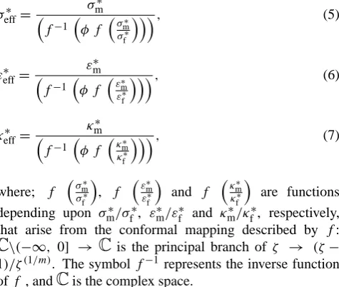
σ_eff∗ = σ

∗

m

f−1_{φ f} σm∗

σ_f∗

, (5)

ε_eff∗ = ε

∗

m

f−1_{φ f} εm∗

ε∗ f

, (6)

κ_eff∗ = κ

∗

m

f−1_{φ f} κ∗m

κ_f∗

, (7)

where; f σ ∗ m

σ∗ f

, f ε

∗ m

ε∗ f

and f κ ∗ m κ∗ f are functions depending upon σ_m∗/σ_f∗, ε∗_m/ε∗_f and κ_m∗/κ_f∗, respectively, that arise from the conformal mapping described by f:

* * * * m eff 1 m f

f

σ

φ

σ

−

=

⎛

⎞

⎜

⎟

⎜

⎝

⎠

⎟

⎝

⎠

,

(5)

* * * * m eff 1 m f

f

ε

φ

ε

−

=

⎛

⎞

⎜

⎟

⎜

⎝

⎠

⎟

⎝

⎠

,

(6)

* * * * m eff 1 m f

f

κ

φ

κ

−

=

⎛

⎞

⎜

⎟

⎜

⎝

⎠

⎟

⎝

⎠

,

(7)

where;

* * m f

f

σ

⎛

⎞

⎜

⎟

⎜

⎟

⎝

⎠

,

* * m f

f

ε

⎛

⎞

⎜

⎟

⎜

⎟

⎝

⎠

and

* * m f

f

κ

⎛

⎞

⎜

⎟

⎜

⎟

⎝

⎠

are functions depending upon

* *

m f

σ σ

,

* *

m f

ε ε

and

* *

m f

κ κ

,

respectively, that arise from the conformal mapping described by f :

^

\ (-

∞

,0]

→

^

is the principal

branch of

ζ

→

(

ζ

– 1)/

ζ

(1/m)

. The symbol f

-1

represents the inverse function of f , and

^

is the complex

space.

A conformal mapping is a transformation

w

=

f z

( )

that preserves local angles. An analytic function is

conformal at any point where it has a nonzero derivative. Conversely, any conformal mapping of a

complex variable which has continuous partial derivatives is analytic. Hence, conformal mapping is

extremely important in many areas of physics and engineering as it allows complex variables to be

converted into an analytically solvable form. By letting

w

≡

f z

( )

, the real and imaginary parts of

( )

w z

must satisfy the Cauchy-Riemann equations and Laplace's equation, so they automatically provide

a scalar potential and a so-called stream function. If a physical problem can be found for which the

\(−∞, 0] → * * * * m eff 1 m f

f

σ

φ

σ

−

=

⎛

⎞

⎜

⎟

⎜

⎝

⎠

⎟

⎝

⎠

,

(5)

* * * * m eff 1 m f

f

ε

φ

ε

−

=

⎛

⎞

⎜

⎟

⎜

⎝

⎠

⎟

⎝

⎠

,

(6)

* * * * m eff 1 m f

f

κ

φ

κ

−

=

⎛

⎞

⎜

⎟

⎜

⎝

⎠

⎟

⎝

⎠

,

(7)

where;

* * m f

f

σ

⎛

⎞

⎜

⎟

⎜

⎟

⎝

⎠

,

* * m f

f

ε

⎛

⎞

⎜

⎟

⎜

⎟

⎝

⎠

and

* * m f

f

κ

⎛

⎞

⎜

⎟

⎜

⎟

⎝

⎠

* *

m f

σ σ

,

* *

m f

ε ε

and

* *

m f

κ κ

,

respectively, that arise from the conformal mapping described by

f :

^

\ (-

∞

,0]

→

^

is the principal

branch of

ζ

→

(

ζ

– 1)/

ζ

(1/m)

. The symbol f

-1

^

is the complex

space.

w

=

f z

( )

conformal at any point where it has a nonzero derivative. Conversely, any conformal mapping of a

extremely important in many areas of physics and engineering as it allows complex variables to be

w

≡

f z

( )

w z

must satisfy the Cauchy-Riemann equations and Laplace's equation, so they automatically provide

a scalar potential and a so-called stream function. If a physical problem can be found for which the

is the principal branch of ζ → (ζ−

1)/ζ(1/m). The symbolf−1represents the inverse function off , and

* * * * m eff 1 m f

f

σ

φ

σ

−

=

⎛

⎞

⎜

⎟

⎜

⎝

⎠

⎟

⎝

⎠

,

(5)

* * * * m eff 1 m f

f

ε

φ

ε

−

=

⎛

⎞

⎜

⎟

⎜

⎝

⎠

⎟

⎝

⎠

,

(6)

* * * * m eff 1 m f

f

κ

φ

κ

−

=

⎛

⎞

⎜

⎟

⎜

⎝

⎠

⎟

⎝

⎠

,

(7)

where;

* * m f

f

σ

⎛

⎞

⎜

⎟

⎜

⎟

⎝

⎠

,

* * m f

f

ε

⎛

⎞

⎜

⎟

⎜

⎟

⎝

⎠

and

* * m f

f

κ

⎛

⎞

⎜

⎟

⎜

⎟

⎝

⎠

* *

m f

σ σ

,

* *

m f

ε ε

and

* *

m f

κ κ

,

respectively, that arise from the conformal mapping described by

f :

^

\ (-

∞

,0]

→

^

is the principal

branch of

ζ

→

(

ζ

– 1)/

ζ

(1/m)

. The symbol f

-1

^

is the complex

space.

w

=

f z

( )

conformal at any point where it has a nonzero derivative. Conversely, any conformal mapping of a

extremely important in many areas of physics and engineering as it allows complex variables to be

w

≡

f z

( )

w z

must satisfy the Cauchy-Riemann equations and Laplace's equation, so they automatically provide

is the complex space.

A conformal mapping is a transformation w=f (z) that preserves local angles. An analytic function is conformal at any point where it has a nonzero derivative. Conversely, any conformal mapping of a complex variable which has continu-ous partial derivatives is analytic. Hence, conformal mapping is extremely important in many areas of physics and engi-neering as it allows complex variables to be converted into an analytically solvable form. By lettingw ≡f (z), the real and imaginary parts ofw(z) must satisfy the Cauchy-Riemann equations and Laplace’s equation, so they automatically pro-vide a scalar potential and a so-called stream function. If a physical problem can be found for which the solution is valid,

Figure 1.

Code required to run the conformal mapping solution.

Maple 11 implementation

Solution of BHS Equation

> BHS:=proc(km,kw,m,phi2)

> local f,finv:

> f:=z->evalf((z-1)/z^(1/m)):

> finv:=w->fsolve(f(z)-w,z):

> km/finv(phi2*f(km/kw)):

End Procedure

> end proc;

Fig. 1. Code required to run the conformal mapping solution.

we obtain a solution, which may have been very difficult to obtain directly, by working backwards.

The implementation of this solution in MapleTM code is given as Fig. 1. It is worth noting that there are only three active lines in the code, which is extremely efficient.

4 Testing

A number of validation tests have been carried out on the method. In all tests we have used conductivities, but note that replacement of the conductivity parameters with relative or absolute permittivities is equally valid. Hence the follow-ing results apply equally to usfollow-ing the Bussian equation and the conformal mapping method with relative or absolute per-mittivities.

In the first test we have examined that the method pro-vides the same results as the Bussian equation for a set of limiting values. The limits of the Bussian equation by math-ematical analysis are set out in Table 1, together with the results of the bisection method and the conformal mapping approach, as well as the physical limits that one might expect for a saturated rock. It should be noted that both the bisec-tion method and the conformal mapping method provide the same limiting results as the mathematical analysis indicates except forσm → ∞, where both the bisection method and

the conformal mapping approach has difficulty in providing a root. This is more likely to be a problem with the internal solver routines of MapleTM 11 than the conformal mapping method itself, but does not impose a significant restriction because applications in this limit are negligible. The limiting solutions indicate that the results of the conformal mapping method are consistent with the Bussian equation.

The question arises whether the Bussian equation accu-rately describes the physical situation. The two cases where σm → 0 and σf → 0 are interesting because although

both the conformal mapping method and classical bisection method provide the result one would expect from taking the

(4)

Table 1. Limiting values of the Bussian equation solutions.

Limit By mathematical From the classical bisection Physical constraints

analysis and conformal mapping methods

φ → 0 σeff → σm σeff → σm σeff →σm

φ = 1 σeff=σf σeff=σf σeff=σf

σm →0 σeff → 0 σeff → 0 σeff →σfφm

σm → ∞ σeff → ∞ No solution σeff → ∞

σf →0 σeff → 0 σeff → 0 σeff →σm(1−φ)m

σf → ∞ σeff → 0 σeff → 0 σeff → ∞

σf=σm σeff=σf=σm σeff=σf=σm σeff=σf=σm

m→ 0 σeff → σf σeff → σf σeff →σf

m= 1 σeff=σfφ+σm(1−φ) σeff=σfφ+σm(1−φ) σeff=σfφ+σm(1−φ)

m→ ∞ σeff → σm

1−φ

_σ

f−σm

σ_f

σ_eff →

σm

1−φ

_σ

f−σm

σ_f

σ_eff →σmwhenφ= 0

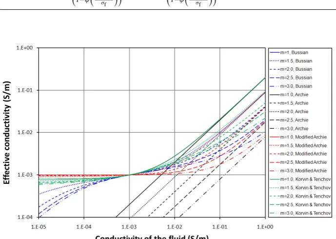
Figure 2. Effective electrical conductivity σeff calculated as a function of porosity at 1001 points for the

Bussian equation (blue) using the conformal mapping method, Archie`s law (black), Modified Archie`s

law (red) and the model of Korvin and Tenchov (green); all for φ = 0.2; m = 1, 1.5, 2, 2.5, 3; σm = 10-3

S/m; 10-5_S/m_≤_σ

f ≤ 1 S/m). Note that all methods except Archie`s law converge atσeff σf 103

− = = S/m.

Fig. 2. Effective electrical conductivityσeff calculated as a function of porosity at 1001 points for the Bussian equation (blue) using the

conformal mapping method, Archie’s law (black), Modified Archie’s law (red) and the model of Korvin and Tenchov (green); all forφ= 0.2; m= 1, 1.5, 2, 2.5, 3;σm= 10−3S/m; 10−5S/m≤σf≤1 S/m). Note that all methods except Archie’s law converge atσeff=σf= 10−3S/m.

mathematical limit of the Bussian equation, that limit is not reasonable from a physical point of view. These two limit-ing cases show a faillimit-ing in the Bussian equation that makes it invalid at low fluid conductivities or low matrix conductivi-ties. The failure, which is due to its derivation from effective medium theory, can be seen clearly in Fig. 2. This figure compares that Bussian equation with Archie’s law (Archie, 1942), the modified Archie’s law (Glover et al., 2000a) and the Korvin and Tenchov method (Korvin, 1982; Tenchov, 1998). Asσf → 0, the effective conductivity should tend

towards a value defined by the porosity, cementation expo-nent and the conductivity of the matrixσeff → σm(1−φ)m,

whereas it is clear in the figure that the Bussian solution tends towards zero like the classical Archie’s law. The other two

curves in Fig. 2 are the solutions by Korvin and Tenchov method (Korvin, 1982; Tenchov, 1998) and by the modified Archie’s law (Glover et al., 2000a). Both of these methods work better than the Bussian equation in the limitσf → 0,

while the modified Archie’s law provides the exact limiting value. Note that all three models are all in fairly good agree-ment forσf ≥ σm.

In the second test we have compared the method with the classical bisection method for a loop that requires the cal-culation of 1001 datapoints, where a datapoint represents a set of solution parameters (i.e., [εm,εf,φandm], [κm,κf,φ

andm] or [σm,σf,φandm]). In our case we chose to

op-erate with conductivities rather than permittivities. We kept the porosity (φ= 0.2), cementation exponent, (m= 1, 1.5, 2,

(5)

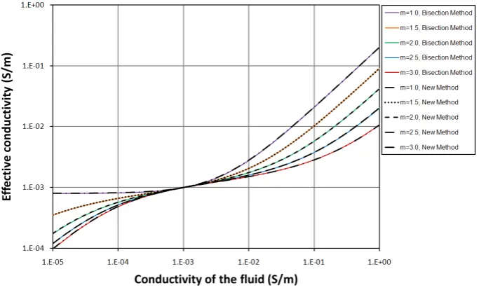
Figure 3. Effective electrical conductivity σeff calculated using the Bussian equation as a function of

porosity at 1001 points for both the bisectionmethod and the conformal mapping method (φ = 0.2; m =

1, 1.5, 2, 2.5, 3; σm = 10-3 S/m; 10-5 S/m ≤σf ≤ 1 S/m). Note that the bisection method and the conformal

mapping method are indistinguishable for all values of φ, m, σm , σf used: A graph of one versus the

other is a 1:1 straight line.

Fig. 3. Effective electrical conductivityσeff calculated using the Bussian equation as a function of porosity at 1001 points for both the

bisection method and the conformal mapping method (φ= 0.2;m= 1, 1.5, 2, 2.5, 3;σm= 10−3S/m; 10−5S/m≤σf≤1 S/m). Note that the

bisection method and the conformal mapping method are indistinguishable for all values ofφ,m,σm,σfused: A graph of one versus the

other is a 1:1 straight line.

2.5, 3.0) and matrix conductivity (σm= 10−3S/m) constant,

and made a calculation for 1001 different values of fluid con-ductivity from 1×10−5S/m to 1 S/m with twenty points per decade, distributed logarithmically. The results of the tests are shown in Fig. 3. It can be seen that both tests perform well insofar as they qualitatively produce the same results (i.e., their curves are indistinguishable). It is impossible to compare each method against a known solution, however, this test validates the conformal mapping method against a well known and respected method that is considered to be extremely robust.

On a more quantitative basis, correlation tests be-tween the results obtained using the classical bisec-tion method and the conformal mapping method that are given in Fig. 3, show them to be statistically the same with a covariance of (3.66±6.19)×10−4S2/m2, a value of 1−r= (5.96±1.14)×10−14, and a value of 1−

r2= (11.92±2.28)×10−14, whereris the correlation coef-ficient andr2is the coefficient of determination. Please note that the values 1−r and 1−r2have been used because the correlation coefficient and coefficient of determination are, respectively, too close to unity to be written down effectively with precision. In these statistics, the values represent the mean calculations from each of the 5 tests for 5 differentm values that are shown in Fig. 3, and the uncertainties repre-sent the standard deviations calculated from those measure-ments. Applying Student’sttest is a trivial exercise because the correlation coefficients are so close to unity. The similar-ity in the precision of the results from the two methods de-rives from setting values of precision and maximum number of iterations in the classical bisection method that correspond

to those implicit in the MapleTM11 solution code. This sim-ilarity of precision allows makes a direct comparison of the speed of the two methods meaningful.

Consequently, we have measured the time required to carry out the calculation of 1001 data points. The results depend upon the values of the input parameters. The results, which are given as a mean over 12 runs±standard deviation, are given in Table 2.

The classical bisection method required between 220.69 and 280.36 s for real data depending on the value of the cementation exponent. It was fastest for m= 1, slightly slower for integer values of m and slowest when the cementation exponent was not an integer. The classical bisection method cannot be used to solve Bussian’s equation if any of the input parameters are complex. By comparison, the conformal mapping method required between 3.46 and 5.41 s for real data, depending on the value of the exponent m, and between 4.02 and 27.59 s for complex data, with the time depending once again on the value of the exponent m. Hence, on elapsed time the conformal mapping method is about 52 times faster than the classical bisection method taking the most general case wheremis not an integer.

Since there is a small but finite computing time associated with the structure of the program (defining variables, report-ing the data etc) we have calculated the mean speed of calcu-lation in the following way. We have run the programme for 1001 datapoints and for 1 datapoint, while retaining the same input parameters, and noting the elapsed time in each case. The mean speed was calculated by subtracting the elapsed time tor 1 datapoint from that for 1001 datapoints and divid-ing by 1000 (i.e., the number of datapoints calculated within

(6)

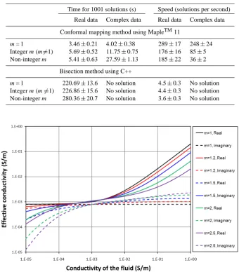
Table 2. Timing tests (mean over 12 runs±standard deviation).

Time for 1001 solutions (s) Speed (solutions per second)

Real data Complex data Real data Complex data

Conformal mapping method using MapleTM11

m= 1 3.46±0.21 4.02±0.38 289±17 248±24

Integerm(m6=1) 5.69±0.52 11.75±0.75 176±16 85±5

Non-integerm 5.41±0.63 27.59±1.13 185±22 36±2

Bisection method using C++

m= 1 220.69±13.6 No solution 4.5±0.3 No solution

Integerm(m6=1) 226.86±15.6 No solution 4.4±0.3 No solution Non-integerm 280.36±20.7 No solution 3.6±0.3 No solution

Figure 4. Complex effective electrical conductivity σeff calculated as a function of porosity at 1001

points for the Bussian equation using the conformal mapping method for φ = 0.2; m = 1, 1.2, 1.5, 2, 2.5;

σm = 10-3+i10-3 S/m; 10-5 S/m ≤σf ≤ 1 S/m).

Fig. 4. Complex effective electrical conductivityσeff calculated as a function of porosity at 1001 points for the Bussian equation using the

conformal mapping method forφ= 0.2;m= 1, 1.2, 1.5, 2, 2.5;σm= 10−3+i10−3S/m; 10−5S/m≤σf≤1 S/m).

the elapsed time difference). The mean speed for the clas-sical bisection method was 3.6±0.3 and 4.5±0.3 solutions per second compared to between 176±16 and 289±17 so-lutions per second needed by the conformal mapping method for real data, and between 36±2 and 248±24 for complex data. Hence for real data the conformal mapping method is 51 times faster than the classical bisection method, again tak-ing the most general case wheremis not an integer.

It is worth noting in Figs. 2 and 3 that all methods ex-cept Archie’s law converge atσeff=σf= 10−3S/m. The

Bus-sian equation provides a reasonable solution in the range σf ≥ σm. However, it should be noted that in this high

salinity range the results provided by the Bussian, Korvin and Tenchov and the Modified Archie’s method provide different results.

Finally, Fig. 4 shows an example of the conformal map-ping method being used to solve the Bussian equation with complex input parameters. In this figure the matrix conduc-tivity is complexσm= 10−3+i10−3S/m, the pore fluid varies

in the range 10−5_S/m_≤_σ

f≤1 S/m, for a porosity φ= 0.2,

and for five values of the cementation exponent,m= 1, 1.2, 1.5, 2, 2.5. It is no longer true thatσeff=σf= 10−3S/m. It is

also worth noting that the solution of Bussian’s equation in complex space suffers from the same difficulties as in the real space when it comes to fluids with low conductivities (i.e., as σf → 0). The innaccuracies in this limit exhibit themselves

both in the real and imaginary parts of the solution and be-come more pronounced asσf → 0 and as the cementation

exponent increases. The problem, as described previously, resides in the formulation of the Bussian equation rather than

(7)

the solution method, and arises due to assumptions that are inherent in the effective medium approach.

It should be noted that the classical bisection method is fairly straightforward to implement under any of the com-mon programming languages, but requires a greater level of programming skill than the conformal mapping implementa-tion in MapleTM11.

It should also be noted that all tests were carried out on a standard desktop PC (Intel Core 2 Quad 2.4 GHz, 4 core, 3 Gb RAM, Microsoft windows XP Professional) running MapleTM11 for the conformal mapping method. The clas-sical bisection method was implemented using the simpli-fied code available in Numerical Recipes in C++: The Art of Scientific Computing, 3rd edition (Press et al., 2007) and Borland C++ 5.5. In both cases the tests were run after a complete reboot of the PC and with no background tasks ac-tive. Elapsed timing was carried out using timestamps for the classical bisection method and using the MapleTM11 native timer. There were no significant usages of physical memory for either method.

5 Conclusions

A new, simple and elegant method for the solution of Bussian equation for the complex effective conductivity, complex di-electric permittivity and complex relative permittivity of two phase mixtures such as water saturated rocks has been devel-oped. The implementation of this method in MapleTM11 al-lows effective and swift solution of these equations. Compar-ison of the conformal mapping method with the classical bi-section method on the same computer shows the new method to be as precise, easier to implement and about 52 times faster to run. The new method is almost as efficient when solv-ing the equation with parameters that are complex numbers, which is something that the bisection method, and the great majority of root finding methods is not capable of doing.

Acknowledgements. This work has been made possible thanks to

funding by the Natural Sciences and Engineering Research Council of Canada (NSERC) Discovery Grant Programme.

Edited by: F. Speranza

References

Acton, F. S.: Numerical Methods that Work, Harper and Row, New York, 1970.

Archie, G. E.: The electrical resistivity log as an aid in determining some reservoir characteristics, Pet. Tech., I, 55–62, 1942.

Bruggeman, D. A. G.: Physikalischer konstanten von het-erogenen Substanzen, Ann. Phys.-Berlin, 24, 636–664, doi:10.1002/ANDP.19374210205, 1935.

Bussian, A. E.: Electrical conductance in a porous media, Geo-physics, 48, 1258–1268, doi:10.1190/1.1441549, 1983. Clavier, C., Coates, G., and Dumanoir, J.: The theoretical and

ex-perimental bases for the “Dual water” model for the interpreta-tion of shaly sands, in SPE 52nd Annual Fall Technical Confer-ence and Exhibition, Denver, 9–12 October, 1977.

de Witte, A. J.: Saturation and porosity from electric logs in shaly sands, Oil Gas J., 55, 89–63, 1957.

Glover, P. W. J., Pous, J., Queralt, P., Mu˜noz, J.-A., Liesa, M. & Hole, M. J.: Integrated two dimensional lithospheric con-ductivity modelling in the Pyrenees using field-scale and lab-oratory measurements, Earth Planet. Sc. Lett., 178, 59-72, doi:10.1016/S0012-821X(00)00066-2, 2000a.

Glover, P. W. J., Hole, M. J., and Pous, J.: A modified Archie’s Law for two conducting phases, Earth Planet. Sc. Lett., 180, 369–383, doi:10.1016/S0012-821X(00)00168-0, 2000b.

Glover, P. W. J.: A generalised Archie’s law fornphases, accepted for publication in Geophysics, 2010.

Gu´eguen, Y. and Palciauskas, V.: Introduction to the Physics of Rocks, Princeton University Press, Princeton, New Jersey, 1994. Hanai, T.: Theory of the dielectric dispersion due to the interfacial polarization and its application to emulsions, Kolloid Z., 171, 23–31, doi:10.1007/BF01520320, 1960a.

Hanai, T.: A remark on the “Theory of the dielectric dispersion due to the interfacial polarization”, Kolloid Z., 175, 61–62, doi:10.1007/BF01520118, 1960b.

Hanai, T.: Dielectric theory on the interfacial polarization for two phase mixtures, Bull. Inst. Chem. Res., 39, 341–367, 1961. Korvin, J.: Axiomatic characterization of the general

mix-ture rules, Geoexploration, 19, 785–796, doi:10.1016/0016-7142(82)90031-X, 1982.

Press, W. H., Teukolsky, S. A., Vetterling, W. T., and Flannery, B. P.: Numerical Recipes: The Art of Scientific Computing, 3rd edi-tion, Cambridge University Press, Cambridge, UK, 2007. Sen, P. N.: The dielectric and conductivity response of sedimentary

rocks, SPE 55th Annual Fall Technical Conference and Exhibi-tion, Dallas, 21–24 September, 1980.

Sen, P. N.: Relation of certain geometrical features to the dielectric anomaly of rocks, Geophysics, 46, 1714–1720, doi:10.1190/1.1441178, 1981.

Sen, P. N., Scala, C., and Cohen, M. H.: Self-similar model for sedimentary rocks with application to the dielec-tric constant of fused glass beads, Geophysics, 46, 781–795, doi:10.1190/1.1441215, 1981.

Tenchov, G. G.: Evaluation of electrical conductivity of shaly sands using the theory of mixtures, J. Petrol. Sci. Eng., 21, 263–271, doi:10.1016/S0920-4105(98)00072-2, 1998.

Waxman, M. H. and Smits, L. J. M.: Electrical conductivities in oil-bearing shaly sand, Soc. Petrol. Eng. J., 8, 107–122, doi:10.2118/1863-A, 1968.

Wyllie, M. R. J. and Southwick, P. F.: An experimental investiga-tion of the SP and resistivity phenomena in dirty sands, J. Petrol. Technol., 6, 44–57, doi:10.2118/302-G, 1954.