https://doi.org/10.5194/cp-15-1771-2019 © Author(s) 2019. This work is distributed under the Creative Commons Attribution 4.0 License.
Objective extraction and analysis of statistical features of
Dansgaard–Oeschger events
Johannes Lohmann and Peter D. Ditlevsen
Physics of Ice, Climate and Earth, Niels Bohr Institute, University of Copenhagen, Denmark
Correspondence:Johannes Lohmann ([email protected])
Received: 6 February 2019 – Discussion started: 25 February 2019
Revised: 21 August 2019 – Accepted: 31 August 2019 – Published: 27 September 2019
Abstract.The strongest mode of centennial to millennial cli-mate variability in the paleoclimatic record is represented by Dansgaard–Oeschger (DO) cycles. Despite decades of research, their dynamics and physical mechanisms remain poorly understood. Valuable insights can be obtained by studying high-resolution Greenland ice core proxies, such as the NGRIP δ18O record. However, conventional statisti-cal analysis is complicated by the high noise level, the cause of which is partly due to glaciological effects unrelated to climate and which is furthermore changing over time. We re-move the high-frequency noise and extract the most robust features of the DO cycles, such as rapid warming and in-terstadial cooling rates, by fitting a consistent piecewise lin-ear model to Greenland ice core records. With statistical hy-pothesis tests we aim to obtain an empirical understanding of what controls the amplitudes and durations of the DO cy-cles. To this end, we investigate distributions and correlations between different features, as well as modulations in time by external climate factors, such as CO2and insolation. Our
analysis suggests different mechanisms underlying warming and cooling transitions due to contrasting distributions and external influences of the stadial and interstadial durations, as well as the fact that the interstadial durations can be pre-dicted to some degree by linear cooling rates already shortly after interstadial onset.
1 Introduction
Different physical mechanism(s) underlying Dansgaard– Oeschger (DO) events have been proposed in the literature. Most of these are characterized by changes between differ-ent modes of operation of the Atlantic Meridional Overturn-ing Circulation (AMOC) that accompany the warm and cold
phases of a DO cycle. This is supported by marine sedi-ment data evidence linking DO cycles and changes in the AMOC (Henry et al., 2016; Lynch-Stieglitz, 2017). Differ-ent drivers for these AMOC changes have been proposed, including North Atlantic freshwater forcing (Ganopolski and Rahmstorf, 2001; Timmermann et al., 2003; Kageyama et al., 2013), variations in ice sheet topography (Zhang et al., 2014), and atmospheric CO2(Zhang et al., 2017). On the other hand,
unforced millennial-scale oscillations involving the AMOC have been reported in comprehensive climate models (Vet-toretti and Peltier, 2016; Klockmann et al., 2018). In these os-cillations, sea ice variability in ocean convection areas plays an important role, which has been proposed previously (Li et al., 2010; Dokken et al., 2013; Petersen et al., 2013) and is supported by recent proxy records (Sadatzki et al., 2019). Another scenario underlying DO cycles might be sponta-neous climate transitions due to extremes in the chaotic at-mospheric dynamics (Drijfhout et al., 2013; Kleppin et al., 2015).
the stadial state. This is referred to as the sawtooth shape of the events.
Due to the high noise level in the record it is, however, difficult to discern this specific structure in all of the events. Some events do not seem to follow the generic shape. Fur-thermore, there are very short events during which it is diffi-cult to speak of a gradual cooling episode. Other events are interrupted by shorter cooling episodes, referred to as sub-events (Capron et al., 2010). As interpretations of noisy time series are often biased, subjective, and prone to the recogni-tion of patterns that can arise by chance, we seek a quantita-tive evaluation of the record. Assuming the sawtooth shape of the events, we develop an algorithm for fitting the sawtooth shape to the entire NGRIP δ18O record of the last glacial, similar to ramp-fitting a jump in a noisy record.
First, our method gives an objective basis of the validity of the generic sawtooth description of the DO cycles and identi-fies which individual cycles fall outside this description. Sec-ondly, with a piecewise linear fit, we obtain estimates for the stadial and interstadial levels, the abruptness of the transi-tions, and the gradual cooling rate in the interstadial periods. By bootstrapping, we estimate the uncertainty in extracting these parameters from the noisy background. Finally, we per-form a comprehensive statistical analysis of the fit parame-ters across the DO events and their relation to external forc-ings in order to obtain an empirical understanding of what controls the evolution of the amplitudes and durations of the DO cycles. This can potentially be used for identifying or ex-cluding proposed mechanisms and for benchmarking model results.
Previous efforts to extract robust DO event features from the record were conducted on only part of the record and were focused on single or very few features. In Schulz (2002), linear fits to the interstadials were used to infer the cooling rates starting with Greenland interstadial 14 (GI-14). Estimates for the abruptness of warming transitions and the durations of interstadials have been derived by Rousseau et al. (2017), starting at GI-17.1. A comprehensive survey of the onset times of all interstadial and stadial periods is given in Rasmussen et al. (2014). Our work is different in that we derive all features that can be extracted from a sawtooth-shaped fit to all events at once by using a fit that is consistent and continuous throughout the record. Thus, our results are not sensitive to subjective choices of cutting the record at predefined times before and after a transition. We do, how-ever, not define the DO events themselves from the NGRIP δ18O record but instead use the set of all previously classified events in Rasmussen et al. (2014), which have been derived from three ice cores and two proxy records each.
In this study, we show that a characteristic sawtooth wave-form can be fit to all DO cycles. However, almost half of the cycles do not actually display a significant rapid cooling episode after the more gradual interstadial cooling. A subse-quent statistical analysis of DO event features hints at differ-ent mechanisms underlying warming and cooling transitions.
First, this follows from the distributions of the durations of the stadials as well as the rapid DO warmings, on the one hand, and of the interstadials on the other hand. Secondly, the influence of external forcing is contrasting, with stronger evi-dence for insolation influence on stadials and CO2or ice
vol-ume influence on interstadials. Thirdly, the interstadial dura-tions can be predicted to some degree by the linear cooling rates within a few hundred years after interstadial onset. In contrast, the stadial and rapid warming durations are consis-tent with the stadial–interstadial transitions as spontaneous, noise-induced escapes from a metastable state.
The paper is structured in the following way: in Sect. 2 we introduce the data used in the study and their preprocessing, the iterative fitting algorithm, the features we extract from the sawtooth-shaped fit to the events, and the statistical tools to analyze these features. In Sect. 3 we report the results of the fit. Section 3.1 discusses the appropriateness of the sawtooth fit to the events, and Sect. 3.2 and 3.3 treat the uncertainty in estimating the fit parameters and the derived features. In Sect. 4 we analyze in detail the features characterizing the stadial, interstadial, and abrupt warming periods. The results of the fit and the implications of the subsequent data analysis are discussed in Sect. 5. We conclude in Sect. 6.
2 Methods and materials
2.1 Data
This study is based on theδ18O Greenland ice core record of the last glacial period (120–12 kyr BP; kyr BP is 1000 years before present). In the NGRIP ice core,δ18O has been mea-sured in 5 cm samples (NGRIP Members, 2004; Gkinis et al., 2014; Rasmussen et al., 2014). The raw depth measurements are transferred to the GICC05 timescale (Svensson et al., 2006), resulting in an unevenly spaced time series with a res-olution of∼3 years at the end to 10 or more years at the beginning of the glacial. To simplify the analysis we trans-fer this to an evenly spaced time series by oversampling to 1-year resolution using nearest-neighbor interpolation. Thus, we do not alter the actually measured values and thus add or remove any variability. For subsequent comparison, the high-resolutionδ18O record from the GRIP ice core on the GICC05 timescale is used (Johnsen et al., 1997; Rasmussen et al., 2014) and processed in the same way.
7. However, they are longer and larger in amplitude. Even though the stadials 23.1 and 14 do not fully reach the val-ues of the stadials before and after, a sawtooth fit whereby these are included in the interstadial is not satisfactory be-cause the resulting gradual linear cooling is not representa-tive of the actual trends. Our choice to consider them as sep-arate events is difficult to justify on the basis of the NGRIP δ18O record alone. Nevertheless, it is unlikely to change the conclusions of our analysis, which are based on statistical robustness tests.
Our analysis uses other datasets that are not derived from Greenland ice cores. These are referred to as external forc-ings, although not all are truly external to the climate sys-tem but rather obtained from independent data sources. As a proxy for global ice volume, we use the LR04 ocean sedi-ment stack (Raymo and Lisiecki, 2005). To represent Antarc-tic temperatures, we choose theδ18O record of the EDML ice core on the AICC12 timescale (EPICA Community Mem-bers, 2010). These data were processed by interpolation to an equidistant 20-year grid and subsequent smoothing with a 600-year Hamming window. Greenhouse gas forcing is rep-resented by a composite CO2record from different
Antarc-tic ice cores on the AICC12 gas timescale (Bereiter et al., 2015a). Furthermore, we consider changes in insolation due to orbital variations. Firstly, we use incoming solar radiation at 65◦N integrated over the summer (referred to as 65Nint hereafter), which we define as the annual sum of the radia-tion on days exceeding an average of 350 W m−2(Huybers, 2006). Secondly, we use incoming solar radiation at 65◦N at summer solstice (referred to as 65Nss hereafter) (Laskar et al., 2004a). In addition, we consider the raw orbital param-eters of obliquity, eccentricity, and precession index (Laskar et al., 2004a).
2.2 Fitting routine
We aim to fit a continuous piecewise linear waveform to the record. This is not possible by simply cutting the time se-ries into DO cycles and fitting each cycle individually be-cause the points at which the time series is cut need to be defined from the fit and in turn influence the fit. Fitting the whole time series at once to a piecewise linear model with 186 parameters, corresponding to 6 parameters for each of the 31 DO events, will be difficult to achieve without invok-ing very complicated constraints because of high noise and an abundance of sub-event features. Instead, we propose the following iterative fitting routine that converges to a consis-tent fit. We start with a guess for the stadial onset and end times, which determine the constant stadial levels. Then we fit a sawtooth shape individually to each event. Thereafter, we update the stadial onset and end times according to the fit and repeat the procedure. When after some iterations the onset and end times do not change significantly anymore, the fit has converged and is consistent.
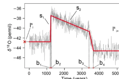
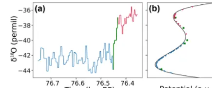
Figure 1.Piecewise linear model fit to DO event 20, for which the time series consists of GS-21.1, GI-20, and GS-20. The parameters of the piecewise linear model are the four break pointsb1,2,3,4, the
up-slopes1, and the down-slopes2. The levelslisandlis+1of
GS-21.1 and GS-20 are constant during an iteration of the fitting routine and are updated after each iteration when all break points have been determined.
The initial guess of the stadial onsets and ends is based on the timings reported by Rasmussen et al. (2014). The time series is divided into segments at these times, which are kept fixed throughout an iteration. For each eventi, we take a seg-ment consisting of a stadial and interstadial period plus the following stadial period. These segments are fitted individ-ually to a piecewise linear model, as shown in Fig. 1. The model starts with a constant line at the beginning of the sta-dial. The constant is fixed to the mean level of the stadiallis, at which the stadial beginnings and ends are determined by the initial guess or the previous iteration. A first break point (parameterb1) of this constant is determined, followed by a
linear up-slope (parameters1). The slope ends at the second
break point (parameterb2). After this break point there is a
linear down-slope (parameters2), which ends at a break point
(parameterb3). After this break point there is a steeper
down-slope until a last break point (parameterb4), which is at the
level of the next stadiallis+1that is determined from the pre-vious iteration. After all events have been fit, the parameters b4 andb1of each event update the beginnings and ends of
the stadials. The updated stadials yield a new segmentation of the time series and new stadial levels, which are then used as constant segments in the next iteration. The hope is that if the problem is well behaved, the beginnings and ends of the stadials do not change significantly anymore after a cer-tain number of iterations, meaning that a consistent fit of the entire time series is obtained. An algorithm for this routine, along with details of the optimization procedure to fit each event, is given in Appendix A.
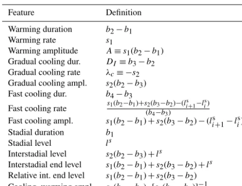
as-Table 1.List of DO event features obtained from the fit that are analyzed in this study.
Feature Definition
Warming duration b2−b1
Warming rate s1
Warming amplitude A≡s1(b2−b1) Gradual cooling dur. DI≡b3−b2 Gradual cooling rate λc≡ −s2 Gradual cooling ampl. s2(b2−b3) Fast cooling dur. b4−b3
Fast cooling rate s1(b2−b1)+s2(b3−b2)−(l s i+1−lsi)
(b4−b3)
Fast cooling ampl. s1(b2−b1)+s2(b3−b2)−(lis+ 1−lis)
Stadial duration b1 Stadial level ls
Interstadial level s2(b2−b3)+ls
Interstadial end level s1(b2−b1)+s2(b3−b2)+ls Relative int. end level s1(b2−b1)+s2(b3−b2) Cooling–warming ampl. s2(b2−b3)· [s1(b2−b1)]−1
sess the uncertainty in each of the parameters that arises due to noise in the record. We cannot estimate this from the out-put of our fitting procedure in a straightforward way. Instead, we use bootstrapping to repeatedly generate synthetic data for each transition and optimize the parameters. Like this, we yield a distribution on each parameter. Due to computa-tional demands, we do not combine this with our iterative procedure but rather resample and fit every transition inde-pendently. Thus, we neglect the covariance structure of the errors in the parameters of neighboring transitions. However, we still consider it to be a very good estimate of the uncer-tainty due to the noise in the record. The detailed procedure is given in Appendix C.
2.3 DO event features
From the best-fit parameters of each DO cycle a variety of features follow. For each rapid warming period, gradual in-terstadial cooling period, and rapid cooling period at the end of an interstadial, we consider the duration, rate of change, and amplitude. Furthermore, several absolute levels are of interest, including the constant stadial levels, the interstadial levels after the abrupt warming, and the interstadial level be-fore the rapid cooling. As a level relative to each event, we consider the level before the rapid cooling above the previous stadial level, which is given by the rapid warming amplitude minus the gradual cooling amplitude. Finally, the gradual cooling amplitude divided by the rapid warming amplitude measures the position of the point of rapid cooling within the event amplitude. In total, we consider 15 interdependent fea-tures, which are listed in Table 1.
2.4 Data analysis
Our aim is to develop an empirical understanding of the evo-lution of the DO cycles. To this end, we employ several tools to search for relations between different features, as well as between features and external climate factors. Ad-ditionally, the distributions of the individual features them-selves hold important information, especially when there is no strong external modulation in time. We test the distribu-tions using Anderson–Darling (AD), Cramér–von Mises, and Kolmogorov–Smirnov tests. Since the AD test is typically the most powerful and the other tests yield qualitatively un-changed results in all of our analyses, we only reportpvalues for the AD test.
Because of the large number of possible combinations of features, we first preselect significant and potentially relevant relationships and thereafter investigate in detail whether the results are robust to outliers, among other things. In some cases we also consider relationships of features and forcings that are not significant for the whole dataset but for a large subset. This might highlight the fact that there were quali-tatively different periods within the last glacial or that some DO events are of a different nature than most.
We first consider Pearson and Spearman correlation co-efficientsrpandrs of pairs of features and external climate
factors. We preselect combinations with p valuesp <0.1, which are estimated by permutation tests that assume inde-pendent samples. For a given number of data points in a se-quence, the truepvalues should often be higher due to auto-correlation. Along with other potential artifacts, this is inves-tigated individually for the preselected combinations.
Next, in order to find relations between more than two variables, we search for multiple linear regression models to explain selected features of the data. Here, we often use log-arithmic quantities because it is otherwise often unlikely to find linear relationships that are not dominated by outliers. Given a feature as a response variable, we consider linear regression models of combinations of two other features or forcings, preselect the models with the largest coefficients of determination, and then further analyze them.
Furthermore, in order to find subsets of events that have distinct properties or relationships that are only valid in part of the data, we perform a clustering analysis on the data using two different algorithms (K-means and agglomerative hier-archical clustering). Given our sample size of 31 events, we search for clusterings with two or three clusters. Clusterings are assessed by considering the mean Silhouette coefficient, which is a distance-based measure for the validity of clus-ters. With the abovementioned tools, we perform an analysis on the entire set of features and forcings. From the results obtained, we report the selected findings that are most robust and relevant in Sect. 4 of this paper.
Spearman correlation yield a non-negligible number of false positives when using confidence levels that are reasonable for our purposes. We consider features of both the same and neighboring events, yielding 152·14=105 and 15·15=225 tests, respectively. Furthermore, we test the correlation of all features and forcings, yielding another 15·8=120 tests. As-suming these are all independent tests, the expected number of false positives is 45 at 90 %, 22.5 at 95 %, and 4.5 at 99 % confidence. Since we derive 15 features from only six inde-pendent parameters for each DO cycle, many pairs of fea-tures are related, and thus we expect true positives for corre-lation tests. For instance, this is true for warming amplitude and interstadial level, as well as relative interstadial level and gradual cooling amplitude. Similarly, due to the constraints on the parameters, the rates and durations of fast and gradual cooling are correlated. These types of correlations are not rel-evant and thus reduce the number of pairwise correlations to consider. For combinations of amplitude, duration, and rates of a given linear segment we also expect correlation because they are trivially related: duration equals amplitude divided by rate. However, it is interesting to test whether the rates or the amplitudes are more strongly correlated with the dura-tions. We investigate this for the different periods of the DO cycles below.
There are sophisticated methods to control the multiple comparisons problem. These could be helpful to better detect false positives from our analysis, but they depend on being able to properly estimate the significance of individual corre-lations between features with autocorrelation and assess the statistical dependence of the hypothesis tests due to the de-pendence of some of the features. For simplicity, we do not consider such an analysis, but we consider individually sig-nificant correlations as suggestions to be investigated further.
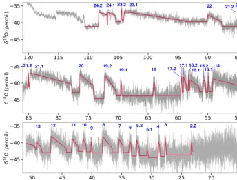
3 Piecewise linear fit of NGRIP record
The fitting routine is performed for 40 iterations so that initial fluctuations in the parameters have died out and converged to a consistent fit, as detailed in Appendix B. Figure 2 superim-poses the resulting fit onto the high-resolution NGRIP time series. We fit 31 DO events in total, starting with DO 24.2 and ending at DO 2.2, excluding the two outermost events of the last glacial because they are very nonstationary in their stadial parts. Table 2 shows all parameters obtained from the fit. Instead ofb1,2,3,4for each transition, we show the
corre-sponding times of stadial end, interstadial onset, interstadial end, and stadial onset.
3.1 Sawtooth shape of DO events
In our fit, all transitions follow the characteristic sawtooth shape. For a few events, this is because of the constraints we use in the fitting algorithm. Typically, the constraints do not strictly bound the best-fit parameters, but they force the fit into another local minimum that is consistent with the
sawtooth shape, which often yields parameters that are still clearly within the constraints. There are, however, four events with parameters close to the bounds. This happens for GI-5.1 and GI-3, which both have ratios of rapid to gradual cooling rates very close to the constraint value of 2.0. Similarly, for GI-15.2 and GI-6 the ratio of gradual to rapid cooling dura-tion is close to 2.0. Detailed pictures of each transidura-tion and the corresponding fit are shown in Fig. S2.
The fact that constraints are needed to ensure that each event follows a sawtooth shape can be used to classify which events fall outside this description. To this end, we perform another run of the iterative fitting routine without using con-straints 3, 4, 6, and 7 listed in Appendix A. From the result-ing fit we then analyze which of the events are not consistent with the sawtooth shape. For this, we use four criteria:
1. the abrupt cooling rate is at least twice as large as the gradual cooling rate;
2. the gradual cooling lasts at least twice as long as the abrupt cooling;
3. there is gradual cooling after the rapid warming, i.e., the gradual cooling rate is negative; and
4. the abrupt cooling amplitude is larger than 0.5 ‰.
Criterion 1 is not met by events 23.1, 19.2, 15.1, 11, 5.1, 3, and 2.2; criterion 2 by events 21.2, 19.2, 17.2, 15.2, 15.1, 11, 10, 9, 8, 6, 5.1, 3, and 2.2; criterion 3 by event 11; and criterion 4 by events 23.1 and 15.1. By demanding that all of these criteria are met, we thus conclude that the following 14 out of 31 events fall outside the sawtooth description: 23.1, 21.2, 19.2, 17.2, 15.2, 15.1, 11, 10, 9, 8, 6, 5.1, 3, and 2.2.
3.2 Uncertainty of fit parameters and features
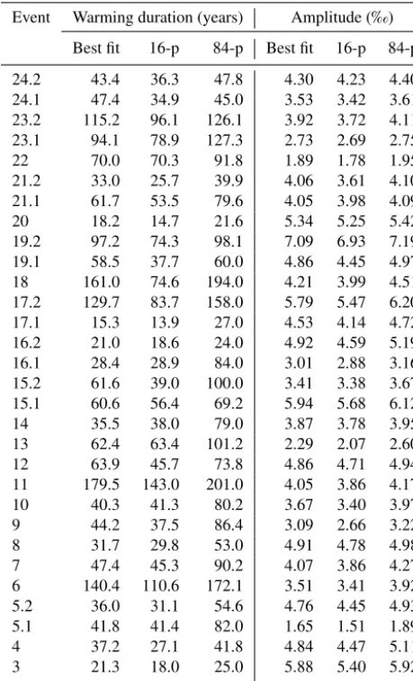
From the best fit, we estimate the uncertainty of each param-eter via bootstrapping, as explained in Appendix C. Distribu-tions of the parameters for DO event 20 are shown in Fig. 3. Table 3 lists the durations and amplitudes of the warmings for each event along with a bootstrap confidence interval consist-ing of the 16th and 84th percentiles, which would correspond to the±σ range if the distributions were Gaussian. The ac-tual distributions are often skewed so that the best-fit values lie close to the edges of the confidence intervals or even out-side the intervals.
Figure 2.High-resolution NGRIPδ18O time series and the piecewise linear fit obtained by our method. The numbers above the interstadials indicate the names of the DO cycles considered in this study.
Figure 3. Gaussian kernel density of the model parameters and some derived quantities for the DO event 20 after 5000 iterations of the bootstrap resampling procedure. The parameter values for the best fit, as reported in Sect. 3, are indicated with red dashed lines. The amplitude feature is given bys1(b2−b1).
with a minimum of 4.6 years for GI-16.2 and a maximum of 209.9 years for GI-23.1. Similarly, the onset times of the rapid warmings have an average bootstrap standard deviation of 11.4 years, whereas the stadial onsets have a correspond-ing average uncertainty of 31.7 years.
3.3 Comparison of NGRIP and GRIP records
As a complementary approach to assess the uncertainties of the features, we compare them to those derived in the same way from another Greenland ice core. We chose theδ18O record of the GRIP ice core, which is measured at a similar resolution to the NGRIP record and has been transferred to the GICC05 timescale starting at the onset of GI-23-1. We fit the record with 40 iterations of our algorithm using the same constraints and hyperparameters. Again, the algorithm converges to a consistent fit, wherein each of the events is well approximated by a sawtooth shape. We now describe how well the features of NGRIP and GRIP correspond for the 26 mutual events starting at GS-22.
For the gradual cooling rates we findrp=0.64 andrs=
0.65. Here, the discrepancy is only due to a handful of short events that show a clear linear cooling slope in one record but are more plateau-like in the other. This happens for the inter-stadials 18, 16.2, and 5.1, which do not show a slope in GRIP, and 17.2, which does not show a strong slope in NGRIP. Removing these events yieldsrp=0.97 andrs=0.98. The
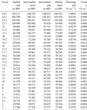
Table 2.Parameters resulting from the fitting routine on the NGRIP data.
Event Stadial Interstadial Interstadial Stadial Warming Cooling end onset end onset rate rate (yr BP) (yr BP) (yr BP) (yr BP) (‰ yr−1) (‰ yr−1) 24.2 108 313 108 270 106 914 106 810 0.0992 0.00062 24.1 106 790 106 743 105 452 105 439 0.0744 0.00069 23.2 104 556 104 441 104 387 104 366 0.0340 0.01555 23.1 104 090 103 996 93 916 93 898 0.0290 0.00027 22 90 069 89 999 87 743 87 631 0.0270 0.00082 21.2 85 060 85 027 84 964 84 952 0.1230 0.03992 21.1 84 799 84 737 77 866 77 659 0.0655 0.00049 20 76 452 76 434 74 245 74 009 0.2935 0.00148 19.2 72 377 72 280 70 385 70 365 0.0730 0.00251 19.1 69 646 69 587 69 443 69 381 0.0831 0.01262 18 64 212 64 051 63 858 63 846 0.0262 0.00367 17.2 59 520 59 390 59 323 59 294 0.0446 0.00503 17.1 59 076 59 061 58 571 58 549 0.2951 0.00491 16.2 58 266 58 245 58 168 58 162 0.2340 0.03107 16.1 58 051 58 023 56 536 56 364 0.1059 0.00131 15.2 55 821 55 759 55 449 55 296 0.0554 0.00062 15.1 55 011 54 950 54 892 54 887 0.0981 0.05104 14 54 228 54 193 49 617 49 410 0.1092 0.00046 13 49 315 49 253 48 517 48 301 0.0367 0.00223 12 46 890 46 826 44 286 44 277 0.0761 0.00140 11 43 450 43 271 42 285 42 278 0.0225 0.00236 10 41 479 41 439 41 024 40 864 0.0910 0.00326 9 40 175 40 131 39 933 39 928 0.0699 0.01096 8 38 231 38 199 36 602 36 583 0.1549 0.00210 7 35 508 35 461 34 741 34 735 0.0859 0.00289 6 33 822 33 681 33 434 33 314 0.0250 0.00334 5.2 32 521 32 485 32 039 32 028 0.1324 0.00583 5.1 30 794 30 752 30 514 30 473 0.0394 0.00695 4 28 908 28 871 28 635 28 544 0.1302 0.00485 3 27 786 27 765 27 572 27 492 0.2762 0.01529 2.2 23 389 23 328 23 196 23 191 0.0607 0.01098
no outliers, but there is a rather large spread, indicating that the warming duration is a less robust feature compared to the cooling rate. With 69 years on average, the GRIP warmings are 8 years shorter than in NGRIP. The average absolute de-viation of warming durations in the two cores is 31 years, with a maximum discrepancy of 103 years for GI-10, with 40 years in NGRIP and 143 years in GRIP. Such deviations can arise if there is a slight step in the record before the most rapid warming and the algorithm includes this in the fit.
The warming amplitudes are very well correlated with rp=0.87 andrs=0.83. The average amplitude of 3.87 ‰
in GRIP is 0.45 ‰ lower than in NGRIP. The stadial levels are also well correlated withrp=0.78 andrs=0.66. There
is a quite consistent offset between the cores of 1.84 ‰ due to differences in altitude and latitude of the GRIP and NGRIP sites. Exceptions include GS-21.1, which does not follow the offset but is at a similar level in both GRIP and NGRIP, and
GS-14, which is difficult to define and thus vulnerable to give different results due to different noise in the cores.
The rapid cooling durations, i.e.,b4−b3, show an
aver-age absolute deviation between the two cores of 59 years, withrp=0.46 andrs=0.53. This corroborates the fact that
this feature is harder to define than the rapid warmings. The break pointsb3andb4are very susceptible to noise and can
yield qualitatively different results for different cores. As a result, the abrupt cooling of GI-19.2 lasts 208 (20) years in GRIP (NGRIP), and for GI-12 it lasts 294 (9) years in GRIP (NGRIP). Conversely, the abrupt coolings of 19.1, GI-10, and GI-6 last much longer in NGRIP, with 62, 160, and 120 years in NGRIP versus 2, 5, and 2 years in GRIP, respec-tively. Consequently, we do not report any results concerning the rapid cooling period in this paper.
The stadial and interstadial durations are very well cor-related with rs=0.99 and rs=0.97, respectively. The
Table 3.Durations and amplitudes of the rapid warmings inferred from the fit, together with a confidence interval obtained by boot-strapping.
Event Warming duration (years) Amplitude (‰) Best fit 16-p 84-p Best fit 16-p 84-p 24.2 43.4 36.3 47.8 4.30 4.23 4.40 24.1 47.4 34.9 45.0 3.53 3.42 3.61 23.2 115.2 96.1 126.1 3.92 3.72 4.11 23.1 94.1 78.9 127.3 2.73 2.69 2.75 22 70.0 70.3 91.8 1.89 1.78 1.95 21.2 33.0 25.7 39.9 4.06 3.61 4.10 21.1 61.7 53.5 79.6 4.05 3.98 4.09 20 18.2 14.7 21.6 5.34 5.25 5.42 19.2 97.2 74.3 98.1 7.09 6.93 7.19 19.1 58.5 37.7 60.0 4.86 4.45 4.97 18 161.0 74.6 194.0 4.21 3.99 4.51 17.2 129.7 83.7 158.0 5.79 5.47 6.20 17.1 15.3 13.9 27.0 4.53 4.14 4.72 16.2 21.0 18.6 24.0 4.92 4.59 5.19 16.1 28.4 28.9 84.0 3.01 2.88 3.16 15.2 61.6 39.0 100.0 3.41 3.38 3.67 15.1 60.6 56.4 69.2 5.94 5.68 6.12 14 35.5 38.0 79.0 3.87 3.78 3.95 13 62.4 63.4 101.2 2.29 2.07 2.60 12 63.9 45.7 73.8 4.86 4.71 4.94 11 179.5 143.0 201.0 4.05 3.86 4.17 10 40.3 41.3 80.2 3.67 3.40 3.97 9 44.2 37.5 86.4 3.09 2.66 3.22 8 31.7 29.8 53.0 4.91 4.78 4.98 7 47.4 45.3 90.2 4.07 3.86 4.27 6 140.4 110.6 172.1 3.51 3.41 3.92 5.2 36.0 31.1 54.6 4.76 4.45 4.93 5.1 41.8 41.4 82.0 1.65 1.51 1.89 4 37.2 27.1 41.8 4.84 4.47 5.11 3 21.3 18.0 25.0 5.88 5.40 5.92 2.2 61.2 42.0 91.6 3.72 3.21 3.75
73 years for stadials, which is small compared to the average durations. The biggest discrepancies between the two cores come from the indeterminacy in the rapid coolings of certain events, as described above.
In summary, the uncertainties obtained by bootstrapping and by comparison with the GRIP ice core are compatible, giving confidence in the estimates of the former method. The average bootstrap standard deviation of rapid warming and cooling durations is 20 and 54 years, respectively. This com-pares well to the average absolute deviation between GRIP and NGRIP of warming and cooling durations of 31 and 59 years, respectively. The discrepancy of 31 years for warm-ing durations also includes a systematic bias of warmwarm-ings that are 8 years longer on average in GRIP. Thus, the unbi-ased uncertainty is likely even closer to the one obtained by bootstrapping. Shorter-timescale features like rapid warming durations are not fully representative for every single event in
one core. However, the overall trends are consistent, as seen by significant correlation. Features on a longer timescale, such as most of the cooling slopes and stadial levels, as well as the stadial and interstadial durations, are clearly represen-tative.
4 Statistical analysis of DO event features
In Fig. 4 we show histograms of all the DO event features derived from the fit parameters that we consider in this study, as defined in Sect. 2.3. The histograms show that the fea-tures have different types of distributions. Whether an event feature should be considered an independent sample from a distribution depends on whether it shows a significant trend over time. If we consider the event-wise sequence of one fea-ture to be an evenly spaced time series we can calculate the autocorrelation and determine by a permutation test whether the value at a given lag is significantly larger than what could be expected in an uncorrelated sample for a given confidence. By considering autocorrelations up to lag 5, we find that the three different levels (stadial, interstadial, and level before rapid cooling) show significant autocorrelation at 95 % con-fidence until a lag of 3. We also find significant autocorre-lation for four other features at only one specific lag value each, which we believe are false positives. When indepen-dently testing the hypothesis of significant autocorrelation at 95 % confidence for 15 different time series (features) at 5 lags, there is an expected value of 3.75 false positives. The corresponding data are shown in Fig. S3. As a result, in most cases we can consider the features of each event to be in-dependent samples. This helps to assess the significance of correlations between features with permutation tests. A gen-eral overview of the correlations between different features and forcings can be seen in Fig. 5 and is explained further in Appendix D. The most important results of our statistical analysis are presented in the following sections.
4.1 Interstadial periods
4.1.1 Relationship of cooling rates, amplitudes, and durations
We focus on the factors influencing the durations of the in-terstadial periodsDI=b3−b2. In our fit, these durations are
furthermore defined byDI =Aλ−c1, whereA is the
ampli-tude andλcthe rate of the gradual cooling. If for every
inter-stadial the gradual cooling were perfectly linear and the jump to stadial conditions always occurred after the same ampli-tude of coolingA, the duration would be inversely propor-tional to the cooling rateDI=Aλ−c1. Conversely, if the
in-terstadials had a fixed cooling rateλcand the jump to stadial
conditions happened after variable cooling magnitudes, the durations would be proportional to the cooling amplitudes DI=Aλ
Figure 4.Histograms of our sample of 31 events for all features considered in this study, as defined in Table 1. The red curves in(b)and
(e)are fits with the exponential and Gumbel distributions, respectively, whereas those in(g)and(n)are fits with the lognormal distribution.
We test which of the two scenarios is better supported by the data. This depends on whether the cooling ampli-tudes or the cooling rates have a larger spread than the other. The coefficient of variation for the amplitudes is CV=0.51, whereas for the rates we find CV=1.49. The correlation of durations and cooling rates (rs= −0.89) is clearly significant
given the sample size of 31 events and weak autocorrelation of the sequence of interstadial durations and rates. This con-firms and extends the finding by Schulz (2002) to the whole glacial period. On the other hand, for durations and cooling amplitudes we find rs=0.40, which is mainly due to two
outliers: the two longest interstadials GI-23.1 and GI-21.1. Removing these reduces the correlation tors=0.30, which
is not significant at 95 % confidence. As a result, there is no relationship between durations and amplitudes that goes be-yond outlier events as opposed to durations and cooling rates. Furthermore, the correlation of cooling amplitudes and rates is not significant.
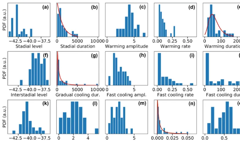
In Fig. 6a we show a scatterplot of logλcand logDIalong
with a linear regression yielding a slope of−0.94. The 95 % confidence interval of this slope obtained via bootstrapping is [−1.12,−0.75]. Because we do not account for errors in the rates estimated from the data the regressed slope is biased to-wards 0 due to attenuation and the true slope will be closer to −1. The modelDI∝λ−c1is consistent with the data, wherein
the spread is caused by the fact that the jump back to stadial conditions happens after varying cooling amplitudes, which have a mean of 2.04 and standard deviation of 1.04.
4.1.2 Distribution of interstadial cooling rates and durations
The relationship between interstadial durations and cooling rates also manifests itself in the respective distributions. As seen in Fig. 4g and n, both features are strongly skewed. Both are consistent with lognormal distributions, withp= 0.47 and p=0.89 for durations and rates, respectively. A fit with this distribution is illustrated in the figure. Because the two features are approximately inversely related with DI=A·λ−c1, the fact that one is a lognormal random variable
implies that the other is, too. IfDI is distributed lognormally
with parametersµandσ, thenλ−c1follows a lognormal dis-tribution with parameters−µ+ln(A) andσ. In our data this relation holds: we estimateµ andσ from the dataDI and
use the observed average amplitudeA=2.04. The dataλ−c1 are consistent (p=0.33) with a lognormal distribution, with −µ+ln(2) andσ.
As opposed to other skewed distributions like exponential, Gumbel, and power law, both durations and cooling rates are also consistent with an inverse Gaussian distribution. The ob-servation that the durations and rates and are both well fitted by the inverse Gaussian despite their inverse relation is ex-plained by the similar shape of the reciprocal inverse Gaus-sian distribution. If a variable is inverse GausGaus-sianX∼IG(x), then the distribution ofY =A
X is reciprocal inverse
Gaus-sianY ∼ A
Figure 5.Spearman correlation heat map of(a)pairs of features within the same DO cycle,(b)pairs of features in adjacent DO cy-cles, and(c) pairs of one feature and one external forcing at the relevant time point of the feature. Correlations that are significant at 95 % (99 %) according to a permutation test are highlighted with a black frame (dot).
Brownian motion with a constant drift. However, the proxy time series in interstadials look qualitatively different than what is expected from this model because they are quite lin-ear and yet have strongly varying slopes. In order for the model to produce roughly linear time series, the drift has to be high, which results in very similar slopes of the time series with the resulting distribution of first hitting times converg-ing to a Gaussian. We leave a further discussion on which mechanism could yield lognormal or inverse Gaussian distri-butions of durations or cooling rates for upcoming studies. Instead, in the following we focus on implications of the ap-proximate linearity of the interstadial time series.
Figure 6.(a)Scatterplot of the logarithms of interstadial durations and cooling rates. The color coding indicates the temporal sequence of the events starting with GI-24.2 as event 0. Two linear fits ob-tained by ordinary least squares are shown. For one of them we fixed the slope to−1 and varied only the intercept.(b)Correlation coeffi-cients of the logarithms of interstadial duration and the linear slope fitted to a slice of the beginning of the interstadial as a function of the length of that slice. The values of the Spearman (Pearson) cor-relation coefficients using slopes obtained from the full interstadials are marked with a dashed (dotted) line.
4.1.3 Predictability of interstadial durations
the length of the slices. The correlation of the slopes esti-mated from the full interstadials and the durations, when ex-cluding events 15.2 and 17.2, isrs=0.94 (rp=0.94) and is
indicated by a dashed (dotted) line. We can see that the cor-relation rapidly increases up to a length of 150 years. There-after the correlation stabilizes until another more rapid in-crease at 350 years. The rapid inin-crease in correlation is partly due to a non-negligible number of events already being at full length (6 events at 150 years and 12 events at 350 years). Still, the slopes of the remaining events also correlate well with the durations. At 350 years, the correlation of the dura-tions with the slopes estimated from the slices is almost as good as with the slopes from the full interstadials. There re-main a handful of longer interstadials (23.2, 22, 14, and 11) that do not settle to a clear negative slope after 350 years. For the latter three events, this is due to sub-events that occur shortly after the interstadial onset.
Our interpretation is that the cooling rate is an indicator of a timescale of large-scale climate reorganization, which can already be measured relatively early in the interstadial and which remains approximately constant. Although we can see that there are exceptions, we conclude that for most events the interstadial duration can be predicted a few hundred years after the rapid warming. Some of the unexplained variance of this prediction is due to other factors influencing the intersta-dial duration that are not diagnosed by the linear cooling rate but, e.g., by the cooling amplitude.
4.1.4 Influence of external forcing
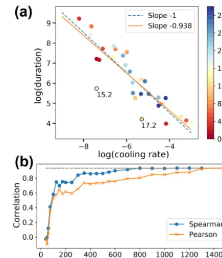
Given the previous result, we investigate whether the vari-ability in the timescale associated with the cooling rate can be explained by other features of the DO cycles or by external forcing. Among correlations of the cooling rates with other features deemed significant by a permutation test, none are relevant, either because they are caused by a few outliers or else directly due to their definition and parameter constraints. Considering external climate factors, we find rs=0.40
and rp=0.35 for the logarithm of the cooling rates with
LR04 at the time of the interstadial maximum. This corre-lation is, however, influenced by a common trend of the two quantities and is not significant anymore at 90 % confidence when removing a linear trend. On the other hand, there is a large subset of events that appears to be linearly related.
As shown in Fig. 7a and c, the furthest outliers from an ap-proximate linear relationship are the interstadials 23.2, 21.2, 16.2, and 15.1. Removing these outliers yields rp=0.79,
which clearly goes beyond a common trend with rp=0.63
after linearly detrending. For the younger half of the record starting with GI-14 we findrp=0.84, corresponding to the
finding by Schulz (2002), who reports that the interstadial cooling rates starting from GI-14 are forced by global sea level. We note, however, that the correlation after GI-14 is largely due to a common trend, as we findrp=0.37 after
lin-ear detrending, which is not significant at 90 % confidence.
Figure 7.(a–b)Scatterplot of the logarithm of the interstadial cool-ing rates and(a)LR04 and(b)EMDL at time points correspond-ing to the interstadial onsets.(c)Time series of the cooling rates (dots) and the LR04 stack (crosses). The error bars on the cooling rates are given by the 16th to 84th percentile obtained by bootstrap-ping.(d)Time series of the cooling rates (dots) and the EDML stack (crosses). Note the inverted axis for EDML.(e)Time series of the interstadial cooling rates starting at GI-14 and of a linear regression model of the CO2record fitted to the logarithm of the cooling rates.
Nevertheless, as shown above, when discarding a few out-liers there is evidence for significant correlation as we in-clude older parts of the record.
A better predictor of the interstadial cooling rates of the more recent DO cycles is given by the CO2composite record.
Whereas for the older half of the glacial there is no significant correlation, when starting at GI-14, we findrp= −0.93 and rp= −0.81 after linear detrending. In Fig. 7e we illustrate
how well the cooling rates of this period can be predicted from CO2by linearly regressing CO2onto the logarithm of
Additionally, in a subset of the events, there is a linear relationship between the logarithm of the cooling rates and EDML at the interstadial onsets. While the entire dataset is not significantly correlated at 90 % confidence (rp= −0.19
and rs= −0.23), removing events 24.2, 23.2, 23.1, 21.2,
16.2, and 15.1 yields an approximately linear relationship, as indicated in Fig. 7b and d. The correlation then becomes rp= −0.81 and rs= −0.78 or rp= −0.72 andrs= −0.61
after linearly detrending, which is significant at 99 % confi-dence. Thus, in this subset there is evidence for anticorrela-tion beyond a simple linear trend. Again, the linear relaanticorrela-tion- relation-ship is strongest for the younger half of the record, which starts at GI-14 and does not have outliers. Here, we find rp= −0.89 andrp= −0.70 after linearly detrending, which
is significant at 99 % confidence.
A corresponding linear relationship between the loga-rithms of interstadial durations and Antarctic temperature in different ice cores has been noted before by Buizert and Schmittner (2015). In our data we find rp=0.29 and rs=
0.27 for these quantities, which is not significant at 90 % confidence. This disagreement comes from the fact that Buiz-ert and Schmittner (2015) view each of the interstadials 24, 23, 21, 17, 16, 15, and 2 as one event, whereas we consider these as two events each, as suggested by the analysis of Rasmussen et al. (2014). Removing the events 24.2, 23.2, 23.1, 21.2, 17.2, 16.2, and 15.1 yields a strong linear rela-tionship ofrp=0.91, comparable to the findings by Buizert
and Schmittner (2015). It is robust to linear detrending with rp=0.87. Most of these outliers are very short events, and
discarding them removes a lot of the variability of the in-terstadial durations, similar to lumping them together with adjacent longer events.
4.2 Stadial periods
4.2.1 Stadial duration distribution
The stadial periods are defined to start after the rapid cooling and end at the onset of the rapid warming, and their dura-tion is thusb1. Due to this definition GS-24.2 is
exception-ally short with 20 years, as the proxy shows rapid warming again right after the rapid cooling without stabilizing. Thus, the durations are highly variable, ranging up to 5169 years for GS-19.1, with an average of 1328 years. The distribution is skewed, as seen in Fig. 4b, where an exponential fit is also given. The data are consistent with an exponential (p=0.79) and a lognormal distribution (p=0.18). Among these two distributions, the exponential is preferred by a relative like-lihood test by a factor of 16. This distribution is relevant for climate dynamics, as it arises in the low noise limit of noise-induced escape times from asymptotically stable equilibria in dynamical systems (Day, 1987).
Figure 8. (a) Scatterplot of stadial levels and logarithmic du-rations. Outliers from an approximate linear relationship are la-beled.(b)Event series of observed stadial levels and those mod-eled byLmod=3.52·X1+98.84·X2−57.96, whereX1is 65Nint
andX2the eccentricity.(c)Models predicting the observed stadial
durations (crosses). The first six events, indicated by gray mark-ers, were discarded when fitting the models. The model based on predicted stadial levels from insolation (squares) is given by log(Dmod)= −0.90·Lmod−32.18. The second model (circles) is
given by log(Dmod)= −0.037·X1−27.11·X2+25.24, whereX1is
65Nss andX2eccentricity. The third model (diamonds) is given by
log(Dmod)= −0.90·X1+75.39·X2+38.71, whereX1is EDML
andX2eccentricity.
4.2.2 Influence of stadial levels and forcing on durations In the following we discuss whether the stadial duration vari-ability is influenced by other features in the data or external factors. Among external factors, the durations are best corre-lated with 65Nss (rs= −0.64). The only DO feature that is
significantly and robustly correlated with the durations is the stadial levels withrs= −0.43. In Fig. 8a we plot the stadial
levels against the logarithms of the durations. If one discards the first six events of the record, there is a linear anticorre-lation ofrp= −0.80 orrp= −0.76 after linear detrending.
This could be either due to common forcing or a direct influ-ence on the durations.
correla-tion with insolacorrela-tion, as seen byrp=0.60 for 65Nss.
Remov-ing the outliers GS-24.2 and GS-22 yieldsrp=0.82, which
does not change when linearly detrending. To see whether this forcing explains most of the correlation of durations and levels, we remove a linear fit to 65Nss from each variable and findrp= −0.38. Even though the significance of this
corre-lation is unclear due to the autocorrecorre-lation of the stadial lev-els, this could imply that there is more information in the stadial levels about the durations than simply common inso-lation forcing. On the other hand, insoinso-lation components in addition to 65Nss might explain more of the observed vari-ability.
We investigate whether multiple linear regression mod-els with two predictors explain the stadial levmod-els and dura-tions better. A model comprised of 65Nint and eccentricity determines the levels very well (R2=0.86), as shown in Fig. 8b. These modeled levels correlate well with the loga-rithm of the stadial durations (rp= −0.64 when excluding
the earliest six events). As model for the durations, we lin-early regress the modeled levels onto the log durations and exponentiate. In Fig. 8c the result is compared to two other models that directly regress external forcings on the log dura-tions. None of the models fits the first six events adequately. Thereafter, all three models produce a similar trend. The model based on predicted stadial levels, and a model with direct forcing by 65Nss and eccentricity, shows similar skill withR2=0.29 andR2=0.30, respectively. The third model based on eccentricity and the EDML record is slightly better withR2=0.46, mainly because it fits two of the longest sta-dials better. Still, all of the models only fit the overall trend, on top of which variability is left unexplained. Unless the correlation is nearly perfect, a linear correlation of the loga-rithm still leaves a lot of room for scatter in the original scale. The exponential tail in the variability of the stadial dura-tions is not a result of the modulation by the external forcings we consider. To demonstrate this, we remove the forcing in-fluence by fitting a linear model of one or more forcings to the log durations. Detrended data are obtained by adding the mean of the logarithmic data to the residuals of the fit and then exponentiating. When using 65Nss as forcing, we find p=0.15 for the exponential distribution. With the model of both eccentricity and 65Nss, as introduced above, we find p=0.29. Thus, the distribution of the detrended data is still long-tailed and consistent with an exponential distribution.
4.2.3 Are stadials with Heinrich events special?
Besides DO events, Heinrich events are the other major mode of glacial millennial-scale climate variability. They corre-spond to massive discharges of ice-rafted debris found in ocean sediment cores (Heinrich, 1988), with large climatic impacts that are well documented in numerous proxy records at various locations. While constraints on their duration and timing need to be improved, we follow Seierstad et al. (2014) for the temporal link of Heinrich events and the GICC05
chronology. This yields the set of Heinrich events H2, H3, H4, H5a, H5, H6, H7a, H7b, and H8, which overlap stadials 3, 5.2, 9, 13, 15.1, 18, 20, 21.1, and 22, respectively. Since some Heinrich events are less established in the community, we also look at the reduced set of H2, H3, H4, H5, and H6.
We test whether these “Heinrich stadials” have signifi-cantly different properties than the remaining stadials, such as longer durations, by randomly sampling nine stadials (five for the reduced set) from the entire set without replacement and calculating the mean duration of this subset. This is re-peated until we can estimate the probability of trials yield-ing a higher mean duration than the actual set of Heinrich stadials. If this is less than 5 % (corresponding top=0.05) we reject the hypothesis that Heinrich stadials have the same mean duration as the remaining stadials at 95 % confidence. This test gives essentially the same results as a one-sidedt test.
For the full (reduced) set of Heinrich events we findp= 0.028 (p=0.022). It is not obvious whether this should be considered significant in the sense of a hypothesis that Hein-rich events prolong stadials. A better statistical test is needed, since if the events were to occur randomly during the course of stadials they would naturally be found preferentially in longer stadials. We leave a resolution of this for upcoming work. Based on the idea that Heinrich stadials are colder than normal, a test on the stadial levels yields p=0.052 (p=0.047). Again, this is probably not significant since Heinrich events mostly occur in the younger glacial with generally lower levels. We can reject the notion that DO events following Heinrich events are “stronger”. A test on the DO warming amplitudes yieldsp=0.102 (p=0.472), whereas a test on the interstadial durations yieldsp=0.403 (p=0.583). This might depend on the precise timing of H3, which in our analysis precedes the especially weak GI-5.1.
4.3 Abrupt warming periods 4.3.1 Warming durations
def-inition of abrupt warmings, we can at least argue that the longest warming transitions are not a result of local noise, because in our fit of the GRIP record the same transitions are also among the longest and clearly above average.
In our analysis we cannot identify any DO cycle fea-tures, external forcings, or combinations thereof that explain a significant part of the variability in the warming durations. Thus, we aim to infer something about the mechanism of the warming transitions from the distribution of their durations. The lognormal (p=0.63), Gumbel (p=0.053), and inverse Gaussian (p=0.95) distributions cannot be rejected at 95 % confidence by the data. A fit with the Gumbel distribution is illustrated in Fig. 4e. The relative likelihood of the Akaike information criterion shows that the inverse Gaussian distri-bution is 9.7 times more likely than the Gumbel distridistri-bution, and the lognormal distribution is 7.6 times more likely than the Gumbel distribution. We cannot choose between lognor-mal and inverse Gaussian with any confidence.
4.3.2 A model for the stadial–interstadial transition In the following we compare the warming durations to what is expected in the framework of noise-induced transitions in multi-stable systems. The DO warmings are much shorter than the time spent in the stadial state. If we consider the stadial–interstadial transition as a noise-induced transition from one metastable state to another, starting at the stadial onset, most of the time is spent in the vicinity of the sta-dial state. The part of the trajectory that leaves this vicinity for the last time and then moves towards the other state (in-terstadial) is referred to as the reactive trajectory. Because of the high noise level in the record, an unknown part of which is non-climatic or regional and changes over time, we do not estimate reactive trajectories by defining neigh-borhoods of two metastable states. Instead, we believe the warming periods obtained by our piecewise linear fit are rea-sonable estimates. Figure 9a illustrates the reactive trajectory (green) leading up to GI-20. In Fig. 9b the different parts of this stadial–interstadial transition are projected onto an arbi-trary potential that features two metastable states. For over-damped motion driven by additive noise in such a potential, it has been proven that the reactive trajectory durations con-verge to a Gumbel distribution in the zero noise limit (Cérou et al., 2013). Similarly, there is numerical evidence for the Gumbel distribution applying to one-dimensional spatially extended systems for low noise (Rolland et al., 2016). Be-cause in our data we cannot separate the true climatic noise potentially driving the observed large-scale climate transi-tions from other types of noise, it is hard to say whether a low noise condition is met and a Gumbel distribution should be expected.
With a small numerical experiment we address the case of finite noise levels and small sample sizes. We use stochas-tic motion in a double-well potential as a generic model for a noise-induced transition from one metastable state to
an-Figure 9.(a)Stadial–interstadial transition leading up to GI-20 (red), including our estimate of the so-called reactive part of the trajectory (green) preceded by 350 years of the stadial GS-21.1.
(b)Data points of the same time series projected onto an arbitrary one-dimensional potential function with two minima as a concep-tual model for the transition.
other. It is given by the stochastic differential equation dXt=
−dV(Xt)
dx
dt+σdWt, with the potentialV(x)=x4−x2and
the Wiener processWt. For zero noise, there are two fixed
points at x= −1 and x=1. We initialize the system at x= −1 and repeatedly collect reactive trajectories, which start when they last leave x <−0.9 and end as they enter x >0.9. Small samples of 31 reactive trajectory durations are indeed typically consistent with a Gumbel distribution for a range of different noise levels, but they can be consistent with other distributions, too.
To show this, we collect p values of AD tests on many small samples. For the Gumbel distribution at a low noise level ofσ=0.00045, 96.3 % of thepvalues are above 0.05. Thus, in this case, very rarely is a sample of 31 reactive tra-jectory durations rejected by a hypothesis test on the Gum-bel distribution. For a higher noise level ofσ =0.5, 80.1 % still yieldp >0.05. However, the lognormal distribution fits equally well, with 95.4 % (93.6 %) yielding p >0.05 for σ=0.00045 (σ=0.5). The distribution that most reliably fits the data is the inverse Gaussian, with>99.9 % (>99.9 %) yielding p >0.05 for σ =0.00045 (σ=0.5), despite the fact that in the zero noise limit the correct distribution is Gumbel. It has been noted that the inverse Gaussian also fits well for large sample sizes (Cérou et al., 2011). Even a non-skewed distribution can be consistent with the samples, as seen for the Gaussian distribution, with 55.1 % (22.8 %) yieldingp >0.05 forσ=0.00045 (σ =0.5). Similar values are obtained for the logistic distribution.
4.3.3 Warming amplitudes
The average amplitude of the warmings is 4.2 ‰, with most events clustering around this value. The most extreme values are 7. ‰ for GI-19.2 and 1.7 ‰ for GI-5.1, which is almost not visually discernible as an event in the δ18O series. The warming amplitudes anticorrelate with the preceding stadial levels. When discarding GI-5.1, this is significant at 99 % confidence withrs= −0.63, which is largely due to GI-19.2
being preceded by a very deep stadial, and 23.1 and GS-22, which are preceded by very shallow stadials, as they hap-pen early in the glacial. When discarding these events the remaining correlation is still significant at 99 % confidence with rs=0.50. Thus, to some degree, the warming
ampli-tudes are predictable in a statistical sense: when residing in a shallow stadial, the amplitude of the next DO warming will be small, and vice versa for a deep stadial. We also assess whether the variability can be explained by external forcing. Our analysis does not show a relationship between the DO amplitudes and global ice volume (LR04), as has been pro-posed by McManus et al. (1999) and Schulz et al. (1999). It should be noted, however, that these studies have a quite dif-ferent notion of DO event amplitudes. Our approach, based on fitting high-resolution data, seems well suited to estimate the actual amplitude of rapid transitions as opposed to low-pass filtering that reduces the amplitude of shorter events. Instead, we find a correlation with 65Nint ofrp= −0.36 and rs= −0.31, which is significant at 90 % confidence.
How-ever, the correlation is visually not striking. Removing GI-19.2, which occurs close to an insolation minimum, yields a correlation that is not significant at 90 % confidence.
5 Discussion
This work presents a statistical analysis of DO event features based on best-fit parameters of a piecewise linear waveform to the NGRIP δ18O record. An assessment of the parame-ter uncertainties shows that some shorparame-ter-timescale features have to be taken with care, such as the rapid warming dura-tions. Here, it is possible that not all individual values are re-liable. However, a comparison with a fit to the GRIP record shows that the overall trends and distributions, also of the shorter-timescale features, are robust. Still, different meth-ods or models to define the features might alter the results. As an example, our piecewise linear method yields quite dif-ferent estimates of the abrupt warming durations compared to Rousseau et al. (2017), wherein abrupt warmings are defined by an estimated derivative of the time series. Our results have an average absolute deviation of 25 years (26 years) com-pared to their algorithmically (visually) determined warming durations starting at GI-17.1.
Furthermore, the work relies on the classification of Greenland ice core centennial to millennial variability into a set of DO events by Rasmussen et al. (2014). This classifica-tion includes short events such as 23.2 and 21.2, which occur
early in the glacial and are surrounded by the longest inter-stadials, as well as 18, 17.2, and 15.2, which are short but do not show a clear gradual cooling. In our analysis, these interstadials frequently show up as outliers. Their presence either showcases the strong irregularity and variability of the processes underlying DO cycles or could indicate that the events are caused by a different trigger and do not represent large-scale reorganizations of the climate system in the same way as longer events. Some of our conclusions might change if all short events were systematically discarded. They do not appear to be local to Greenland, since they are seen in atmospheric methane records (Rhodes et al., 2017) and speleothem records from the Alps (Boch et al., 2011; Mose-ley et al., 2014) and Asia (Cheng et al., 2016). However, their significance in comparison to longer DO events is an open problem that needs to be evaluated as more precisely dated, high-resolution records from outside Greenland be-come available.
Our analysis suggests that the mechanisms underlying warming and cooling transitions are likely different due to contrasting statistical properties. The stadial duration dis-tribution closely resembles an exponential, and its large dispersion cannot be explained by external forcing alone (Sect. 4.2.2). This is expected in systems with noise-induced escape from one metastable state to another (Sect. 4.2.1). Furthermore, the distribution of DO warming durations is also consistent with the durations of so-called reactive trajec-tories in noise-induced transitions (Cérou et al., 2013; Rol-land et al., 2016) (Sect. 4.3.2). Thus, the stadial–interstadial transition, i.e., the stadial plus the rapid warming phase, is consistent with a noise-induced escape from a metastable state and thus with spontaneous, unforced climate transitions, such as the ones observed in Drijfhout et al. (2013) and Klep-pin et al. (2015). However, evidence for a different scenario might arise with new data or analyses, as in the studies by Rypdal (2016) and Boers (2018), who suggest a bifurcation in a fast climate subsystem before DO warmings, evidenced by increases in high-frequency variance of the ice core record prior to some events. If this is the case, it would mean that the transitions are not purely noise-induced but predictable to some degree and potentially part of a self-sustained os-cillation such as in the model experiments by Vettoretti and Peltier (2016) and Klockmann et al. (2018).
from event to event, can be inferred from the cooling rate and stays consistent throughout the interstadial. We suggest that this reorganization is a major driving force of the DO cy-cle because its timescale predicts with reasonable accuracy when the interstadial–stadial transition takes place, which as a result cannot be purely noise-induced.
External forcing might explain the large variability of this timescale, as proposed by Schulz (2002), who argues that the interstadial cooling rates are controlled by global sea level in the younger half of the last glacial. For the older glacial, this relation is weak due to a number of outliers (Sect. 4.1.4). A physical pathway for such a forcing might be the influences of global ice volume on the strength and stability of the inter-stadial (strong) mode of the AMOC. However, climate model studies show that enlargement of Northern Hemisphere ice sheets actually enhances the stability of the strong AMOC state (Zhang et al., 2014; Ullman et al., 2014; Muglia and Schmittner, 2015). Intuitively, this would result in longer in-terstadials, which is in contrast to what the ice core data suggest. This has been addressed by Buizert and Schmittner (2015), wherein Southern Ocean processes are invoked to in-fluence interstadial durations. We find that the correlation of Antarctic temperature and interstadial duration reported in this study is only valid if certain outliers are discarded. Fi-nally, for the younger half of the glacial starting at GI-14, we find that atmospheric CO2is a much better predictor of the
cooling rates. A sensitive dependence of the strong AMOC state on CO2 has been verified in model experiments by
Kawamura et al. (2017). However, more experiments with an active carbon cycle are needed to clarify whether CO2should
be considered forcing or a response to the DO cycle. Yet an-other model showed that changes in CO2could in fact even
be the trigger of DO-type transitions (Zhang et al., 2017). Thus, the influence of external forcing is different for sta-dial and interstasta-dial periods, with more evidence for inso-lation forcing on stadials and ice volume or CO2on
inter-stadials, which is related to the findings by Lohmann and Ditlevsen (2018). Except for a common forcing envelope of stadial and interstadial levels, there is no strong relationship between features across the different periods of the DO cy-cle. As a result, our analysis allows for the interpretation of the DO cycle as a manifestation of an excitable system, as proposed by Ganopolski and Rahmstorf (2002) and Timmer-mann et al. (2003), with a noise-induced transition out of the stadial state to the marginally unstable interstadial state, and a deterministic excursion back to the stadial state. However, the vastly different timescales for this excursion still need an explanation.
6 Conclusions
We developed a method to fit a continuous piecewise linear waveform to the entire last glacial NGRIPδ18O record that can fit a characteristic sawtooth shape to every DO event. However, we find that for many of the transitions this is ad hoc. Almost half of the events do not show a distinct and sig-nificant rapid cooling episode after the more gradual inter-stadial cooling. An analysis of the DO event features derived from the fit confirms the irregularity and randomness that is evident from visual inspection of the record. There is hardly any evidence for relationships linking the features that de-scribe the stadial, interstadial, and abrupt warming periods, except for a common envelope that governs the stadial and interstadial levels via external forcing. A statistical analysis hints at different mechanisms underlying warming and cool-ing transitions. This follows from the distributions of the sta-dial and rapid DO warming durations, on the one hand, and the interstadial durations on the other hand. It is furthermore supported by the different importance of CO2, ice volume,
and insolation forcing to explain the stadial and interstadial properties, as well as the fact that the interstadial durations can be predicted to some degree by the linear cooling rates shortly after interstadial onset.
Data availability. This work is based on the high-resolution NGRIP oxygen isotope record of the entire last glacial period. The data up until 60 kyr BP are available at http://iceandclimate.nbi.ku. dk/data/NGRIP_d18O_and_dust_5cm.xls (last access: 20 Septem-ber 2019) (NGRIP memSeptem-bers, 2015), whereas the older parts of the record are currently in the process of being published by col-leagues at Physics of Ice, Climate and Earth at the University of Copenhagen. Until then, the data can be requested from the authors. The insolation dataset 65Nint is publicly available as supporting online material to Huybers (2006) (doi:10.1126/science.1125249) and the orbital forcing parameters from Laskar et al. (2004b); 65Nss insolation is available at http://vo.imcce.fr/insola/earth/ online/earth/earth.html (last access: 20 September 2019). The ice volume data from Lisiecki and Raymo (2005) are publicly avail-able at https://doi.pangaea.de/10.1594/PANGAEA.704257 (last ac-cess: 20 September 2019). The Antarctic EDML oxygen iso-tope record is available at https://doi.org/10.1594/PANGAEA. 754444 (last access: 20 September 2019) (EPICA Community Members, 2010), whereas the Antarctic composite CO2 record
Appendix A: Iterative algorithm to fit piecewise linear model
In the following, we detail the optimization procedure to find the best sawtooth-shaped fit for each event, i.e., line 18 of the algorithm above. To determine the six parameters at each transition, we minimize the root mean square deviation of the fit from the time series segment. Due to the high noise level, there are many local minima in this optimization prob-lem. Thus, either a brute-force parameter search on a grid or an advanced algorithm is needed to find a global mini-mum. We chose an algorithm called basin-hopping, which is described in Olson et al. (2012) and is included in the Sci-entific Python package scipy.optimize, wherein it can also be customized. The basic idea of the algorithm is the following: given initial coordinates in terms of the parameter vectorθ0,
one searches for a local minimum of the goal functionf(θ), e.g., with a Newton, quasi-Newton, or other method. The ar-gument to this local minimumθnis then randomly perturbed
by a kernel to yield new coordinatesθ∗, which are the starting point of a new local minimization. Next, there is a metropo-lis accept or reject step: we accept the argument of the local minimizationθn+1as new coordinates if the local minimum
is deeper than the previous onef(θn+1)< f(θn), or else with
probabilitye−(f(θn+1)−f(θn))/T, whereT is a parameter
relat-ing to the typical difference in depth of adjacent local min-ima. Now we go back to the perturbation step either with old coordinatesθnor, if accepted, with new coordinatesθn+1and
repeat. The iterative procedure is repeated for a large number of iterations and the result is the argument to the lowest func-tion value found.
Within basin-hopping, one has the freedom of choosing any local minimizer as well as a perturbation kernel. These have to be adapted to our optimization problem. We have sev-eral constraints on the parameters that need to be satisfied by the optimization. For instance, we demand that all segments of the fit are present and do not overlap (b1< b2< b3< b4).
Other constraints ensure that the characteristic shape of DO events is fit as well as possible for all events. Among other things, we thus demand the gradual slope to be significantly longer and less steep than the fast cooling transition at the end of an interstadial. An overview of all the constraints we used is given further below. To satisfy them, we chose a multivariate Gaussian perturbation kernel, which is trun-cated at the respective parameter constraints. The local mini-mizer choice requires further consideration. Our goal func-tion landscape is very rough and not differentiable. Thus, methods like gradient descent give very poor results in our case. A method that does not depend on derivatives and can handle constraints is called constrained optimization by lin-ear approximation (COBYLA), and we found it to work well in our case.
Two hyperparameters have to be specified in the basin-hopping algorithm: the variance of the perturbation kernel and the parameterT used in the metropolis criterion. These should both be comparable to typical differences in goal function (temperature) and arguments (perturbation width) of neighboring local minima in the minimization problem. We chose these parameters empirically by observing how the goal function changes as we slightly change the fit. Although this varies significantly from transition to transition, we de-termined single values as a compromise for all transitions. For the kernel variance in the directions ofb1,2,3,4we chose
a value of 15, and fors1ands2we chose 0.004 and 0.0015,
respectively.