DESIGN OF PI CONTROLLER FOR A CONICAL TANK SYSTEM

Pandimadevi et al. World Journal of Engineering Research and Technology

DESIGN OF PI CONTROLLER FOR A CONICAL TANK SYSTEM

*G. Pandimadevi M. E. and Dr. V. Selvakumar2

Lecturer, Engineering Department, Nizwa College of Technology, Nizwa, Sultanate of

Oman.

Article Received on 15/11/2017 Article Revised on 06/12/2017 Article Accepted on 27/12/2017

ABSTRACT

Conical tanks are widely used in the process industries because of its

shape that contributes better drainage for solid mixtures, slurries and

viscous liquids. The cone is a well-known system, which is having

high non linearity, due to the variation of the area with respect to

height. Level control of conical tank is a challenging task due to its

non-linear shape and constantly varying cross-section. Thus automatic control of such

nonlinear process is a challenging task. To recover the nonlinearity problem dynamics, those

sys-tems should be analyzed properly. This paper proposes the tuning of PI controller by

Ziegler Nicholas and Cohen coon method. The controllers are designed and compared based

on the performance analysis.

KEYWORDS: Ziegler Nicholas, Cohen Coon; Controller; Conical Tank; Simulation.

INTRODUCTION

The common need for accurate and efficient control of today’s industrial applications is

driving the system identification field to face the constant challenges of providing better

models of physical phenomena. Systems encountered in practice are often nonlinear or have

time varying nature. So, it is difficult to identify accurate models of a nonlinear system.

Approximate linear models are used in most of the industrial controllers, which may lead to

lower the control performance. Hence, it is important to develop a simple and practical

method for nonlinear process modeling and identification, and use that model for the control

of nonlinear processes.

World Journal of Engineering Research and Technology

WJERT

www.wjert.org

*Corresponding Author

G. Pandimadevi M. E.

Lecturer, Engineering

Department, Nizwa College

of Technology, Nizwa,

The control of liquid level in tank and flow in the tank is a basic problem in process

industries. The process industries require the liquids to be pumped, stored in tanks and then

pumped to another tank. Many times the liquid will be processed by chemical or mixing

treatment in the tanks, but always the level of the fluid in the tanks must be controlled.

Controlling of liquid level is an important and common task in process industries, in this level

process, the tank is conical shape in which the level of liquid is desired to maintain at a

constant value. The level control in the conical tank is a challenging problem because of its

constantly changing its cross sectional area.[1]

This is achieved by controlling the input flow into the tank. The control variable is the level

in a tank and the manipulated variable is the inflow to the tank. Conical tanks find wide

applications in process industries, namely hydrometallurgical industries, food process

industries, concrete mixing industries and wastewater treatment industries. Conical tank gives

better drainage to the solid materials, semi solid materials as well as viscous fluids. The

Proportional Integral Derivative (PID) Controllers have been widely used in the process

industries for many years, due to their simplicity, flexibility and efficiency.[2] The tuning of a

PID Controller is necessary, for the satisfactory operation of the process. Standard methods

for tuning include, Zeigler-Nichol’s (ZN) ultimate cycling method, and Cohen- Coon’s (CC)

open loop tuning method. In both these methods, the parameters of the controller are obtained

for an operating point, when the plant or process model is linear. This paper focuses on the

design of PI controllers for controlling the level of a conical tank process.

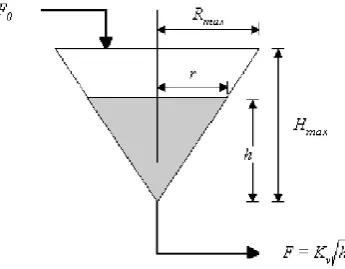
2. PROCESS DESCRIPTION

The conical tank system has single input and single output process. The output of this process

is the level and the input to the process is the flow of liquid. The structure of the conical tank

system is given in fig 1.

A liquid of constant density is fed at a constant volumetric rate Fo into a conical tank of

height Hmax and maximum radius Rmax.The outflow from the tank is , where h is the

height of the liquid in the tank and is the valve coefficient.

The process has high nonlinearity due to the changes in Process gain and time constant with

respect to the height of the liquid tank.[3,4]

Let the inflow (F0), outflow (F). by the mass conservation law,

Mass accumulation = inflow –outflow

Accumulation manifests itself as an increase or decrease in volume.(i.e) Accumulation is the

change in volume with respect to time.

(1)

Right circular cone has volume

(2)

Consider

= (3)

Hence (4)

Therefore

(5)

(6)

(7)

So (8)

The above mathematical model is analyzed in MATLAB Simulink and the responses are

3. PROCESS OPERATING PARAMETERS

The various system parameters[5] obtained are tabulated as:

Table 1: Parameters of Conical-tank system.

Parameter Description Value

Rmax Total radius of the cone 19.25 cm

Hmax Maximum total height of the tank 73 cm

Fo Maximum inflow rate of the tank 400 LPH

Kv Valve Coefficient 55cm2 /s

h Height of the liquid level Varied with the requirement

F Outflow Variable

r Radius at the height h Variable

4. SIMULATION RESULTS

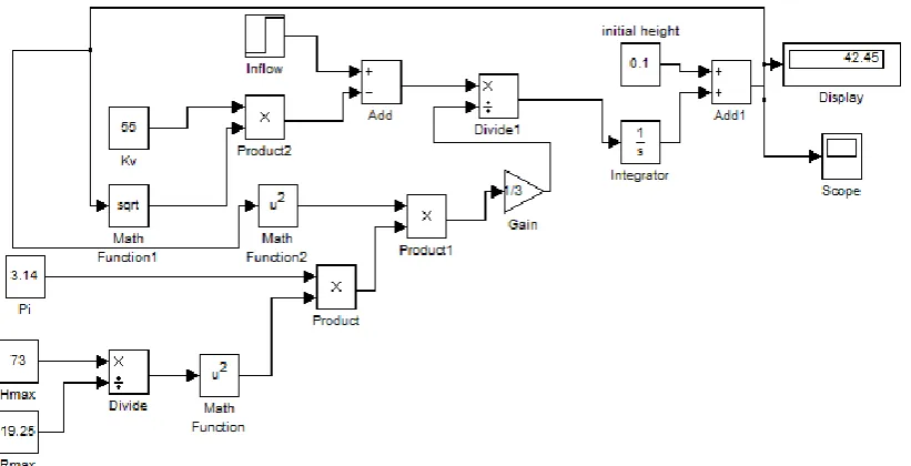
Based on the dynamic equation derived in Mathematical Modelling section, a Simulink block

diagram in figure 2 showing the nonlinear model of the plant is designed in MATLAB. Also

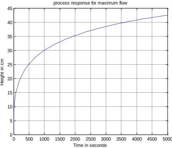
the open loop response of the system is obtained as shown in figure 3.

0 500 1000 1500 2000 2500 3000 3500 4000 4500 5000 0 5 10 15 20 25 30 35 40 45

Time in seconds

H e ig h t in c m

process response for maximum flow

Figure 3: Process input-output characteristic.

To obtain a linear model the characteristic is divided into four different linear regions as

shown in Figure 4.

0 50 100 150 200 250 300 350 400 450 500

0 5 10 15 20 25 30

Piecewise linearized response

H e ig h t in c m

Time in seconds I

II III

IV

Figure 4: Piecewise linearized process input- output characteristic.

A first order mathematical model is then obtained for each region using process reaction

curve method and the reaction curves for regions 1 to 4 are shown in Figures 5 to8. The gain

(K), dead time (td) and time constant (τ) are measured from the reaction curves and are given

0 5 10 15 20 25 30 35 40 45 50 1.3

1.35 1.4 1.45 1.5

Time in seconds

H

e

ig

h

t

in

c

m

Response for Inflow(0-66)LPH

response of model equation

Figure 5: Reaction curve for first region when step change in inflow (0-66)LPH.

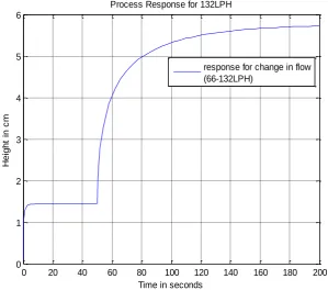
0 20 40 60 80 100 120 140 160 180 200

0 1 2 3 4 5 6

Time in seconds

H

e

ig

h

t

in

c

m

Process Response for 132LPH

response for change in flow (66-132LPH)

0 200 400 600 800 1000 1200 1400 1600 1800 2000 0

2 4 6 8 10 12 14

H

e

ig

h

t

in

c

m

Time in seconds Process Response for 198LPH

Response for change in flow (132-198LPH)

Figure 7: Reaction curve for 3rd region inflow(132-198)LPH.

0 500 1000 1500 2000 2500 3000 3500 4000 4500 5000

0 5 10 15 20 25

Time in seconds

H

e

ig

h

t

in

c

m

Process Response for 264LPH

Response for change in flow (198-264LPH)

Table 2: Process parameters obtained from the reaction curves. Inflow

(LPH)

Time (Seconds)

Height/Level

(cm) Steady state gain

Time constant (Secs)

0-66 0-50 1.44 0.0218 0.002

66-132 50-150 5.76 0.087 0.24

132-198 150-250 12.81 0.194 1.97

198-264 250-500 23 0.348 11.75

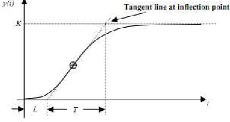
5. CONTROLLER TUNING 5.1 Ziegler Nicholas Method

The Ziegler-Nichols design methods are the most popular methods used in process control to

determine the parameters of a PID controller. Although these methods were presented in the

1940s, they are still widely used. The step response method is based on an open-loop step

response test of the process. Hence requiring the process to be stable, the unit step response

of the process is characterized by two parameters L and T. These are determined by drawing

a tangent line at the inflexion point, where the slope of the step response has its maximum

value. The intersections of the tangent and the coordinate axes give the process parameters as

shown in Figure 9, and these are used in calculating the controller parameters.[6]

Figure 9: Response curve for ZN method.

The parameters for PID controllers obtained from the Ziegler Nichols step response method

are shown in Table 3.

From the MATLAB Simulink model the ZN open loop response is observed and the value of

T, L are obtained and the parameters of Kp and Ki are calculated by using the above table.

The calculated values are Kp=50 and KI =25000.

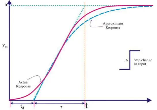
5.2 Cohen Coon Method

The Cohen-Coon method is a more complex version of the Ziegler-Nichols method .This

method is more sensitive than the Ziegler-Nichols method. It is observed that the response of

most of the processes under step change in input yields a sigmoidal shape (figure 10).The

parameters for PID controllers obtained from the Cohen Coon step response method are

shown in Table 4.

Figure 10: Response curve for CC method.

Table 4: Parameters tuned using Closed-Loop CC Method.

From the MATLAB Simulink model the open loop response is observed and the value of K,

Kp and Ki are calculated by using the above table. The calculated values are Kp=492.90 and

KI = = 407547.01.

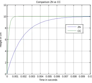
6. RESULTS AND DISCUSSION

The response of Ziegler Nicholas method is compared with the Cohen Coon type tuning. The

comparison graph is shown in figure 11.

0 0.001 0.002 0.003 0.004 0.005 0.006 0.007 0.008 0.009 0.01 0

2 4 6 8 10 12

Comparison ZN vs CC

H

e

ig

h

t

in

c

m

Time in seconds

ZN CC

Figure 12: ZNT v/s CC Response.

The graph shows that the Cohen Coon tuned controller is reaching the set point value in less

time compared to the ZN.The performance of the controllers are analyzed by calculating the

Integral Square Error (ISE), Integral time multiplied by Square Error (ITSE), Integral

Absolute Error (IAE) and Integral time multiplied by absolute Error (ITAE).The obtained

values are tabulated in Table 5.

Table 5: Comparison of ZNT and CC.

Parameter ZNT CC

ISE 0.09161 0.008973

IAE 0.01835 0.002165

ITAE 3.367e-005 1.194e-006

7. CONCLUSION

The conical tank system is identified as a non-linear system. The model of conical tank

system is implemented with the help of first principle differential equation. MATLAB

ODE45 solver/Simulink is used to solve the differential equation. The results are validated by

using the transfer function model and ODE response. The conventional PI controller is

implemented to track the multi set point changes in level of the conical tank process by using

different tuning rules.

The performance index of different tuning rules are also obtained. The simulation results

proven that the Cohen Coon control method is an easy-tuning and more effective way to

enhance stability of time domain performance of the conical tank system.

8. REFERENCES

1. Nithya.S, Abhay Singh.G, Radhakrishnan.T.K, Balasubramanian. T and Anantharaman.

N, “Design of intelligent controller for non-linear process”, Asian Journal of applied

Science, 2008; 1: 33-45.

2. N. S Bhuvaneshwari, G. Uma, T. R. Rangaswamy, Adaptive and optimal control of an

nonlinear process using intelligent controllers, Applied soft computing, 2009; 9: 182-190.

3. B Ziegler, G. and Nichols, N. B,.Optimum settings for automatic controllers, Trans.

ASME, 1942; 64: 759-768.

4. S.Anand, V.Aswin, S.Rakeshkumar, “Simple tuned adaptive PI Controller for conical

tank process” International Conference on Recent Advancements in Electrical,

Electronics and Control Engineering (ICONRAEeCE), 263-267.

5. E.Kesavan, E.Arunkumar, Deivasigamani, “Design of an Adaptive Controller for Non

Linear System”, International Journal of Advanced Research in Electrical, Electronics

and Instrumentation Engineering, 2013; 2(9).

6. P.Aravind, M.Valluvan, S.Ranganathan, “Modelling and Simulation of Non Linear Tank”

International Journal of Advanced Research in Electrical, Electronics and Instrumentation