A New Regularity Lemma and Faster Approximation Algorithms for Low Threshold Rank Graphs

THEORY OFCOMPUTING, Volume 11 (9), 2015, pp. 241–256 www.theoryofcomputing.org

S

: APPROX-RANDOM 2013

A New Regularity Lemma and

Faster Approximation Algorithms for

Low Threshold-Rank Graphs

Shayan Oveis Gharan

Luca Trevisan

Received February 4, 2014; Revised March 27, 2015; Published June 10, 2015

Abstract: Kolla and Tulsiani (2007, 2011) and Arora, Barak and Steurer (2010) introduced the technique ofsubspace enumeration, which gives approximation algorithms for graph problems such as unique games and small set expansion; the running time of such algorithms is exponential in thethreshold rankof the graph.

Guruswami and Sinop (2011, 2012) and Barak, Raghavendra, and Steurer (2011) de-veloped an alternative approach to the design of approximation algorithms for graphs of bounded threshold rank based on semidefinite programming relaxations obtained by using sum-of-squares hierarchy (2000, 2001) and on novel rounding techniques. These algo-rithms are faster than the ones based on subspace enumeration and work on a broad class of problems.

An extended abstract of this paper appeared in the proceedings of the 16th International Workshop on Approximation Algorithms for Combinatorial Optimization Problems (APPROX 2013) [15].

∗_{Department of Computer Science and Engineering, University of Washington.}

†_{Department of Electrical Engineering and Computer Sciences U.C. Berkeley. This material is based upon work supported}

by the National Science Foundation under grant No. CCF 1017403.

ACM Classification:F.2.2, G.2.2, G.1.6

AMS Classification:68W25, 68Q25, 68R10

In this paper we develop a third approach to the design of such algorithms. We show, constructively, that graphs of bounded threshold rank satisfy aweak Szemerédi regularity lemma analogous to the one proved by Frieze and Kannan (1999) for dense graphs. The existence of efficient approximation algorithms is then a consequence of the regularity lemma, as shown by Frieze and Kannan.

Applying our method to the Max Cut problem, we devise an algorithm that is slightly faster than all previous algorithms, and is easier to describe and analyze.

1

Introduction

Kolla and Tulsiani [13,12] and Arora, Barak and Steurer [2] proved that the Unique Games problem can be approximated efficiently if the adjacency matrix of a graph associated with the problem has few large eigenvalues; they show that, for every optimal solution, its indicator vector is close to the subspace spanned by the eigenvectors of the large eigenvalues, and one can find a solution close to an optimal one by enumerating anε-net for such a subspace. This algorithm, also known as thesubspace enumeration algorithm, runs in time exponential in the dimension of the subspace, which is the number of large eigenvalues; the number of large eigenvalues is called thethreshold rankof the graph. Arora, Barak and Steurer show that the subspace enumeration algorithm can approximate other graph problems, in regular graphs, in time exponential in the threshold rank, including the Uniform Sparsest Cut problem, the Small-Set Expansion problem and the Max Cut problem. We remark that the subspace enumeration algorithm does not improve the 0.878 approximation guarantee of Goemans and Williamson [8], but it finds a solution of approximation factor 1−O(ε)if the optimum cuts at least 1−εfraction of edges.

Barak, Raghavendra and Steurer [3] and Guruswami and Sinop [9,10,11] developed an alternative approach to the design of approximation algorithms running in time exponential in the threshold rank. Their algorithms are based on solving semidefinite programming relaxations obtained by using the sum-of-squares hierarchy [16,14] and then applying sophisticated rounding schemes. This approach has several advantages. It is applicable to a more general class of graph problems and constraint satisfaction problems, that the approximation guarantee has a tighter dependency on the threshold used in the definition of threshold rank and that, in some cases, the algorithms have a running time of f(k,ε)·nO(1)wherekis the threshold rank and 1±ε is the approximation guarantee, instead of the running time ofnO(k)which follows from an application of the subspace enumeration algorithm for constantε.

In this paper we introduce a third approach to designing algorithms for graphs of bounded threshold rank, which is based on proving aweak Szemerédi regularity lemmafor such graphs.

time.1 Combining the two facts one has a exp(poly(1/ε)) +poly(n)time approximation algorithm for many graph problems on dense graphs.

We prove that a weak regularity lemma holds for all graphs of bounded threshold rank. Our result is a proper generalization of the weak regularity lemma of Frieze and Kannan, because dense graphs are known to have bounded threshold rank,2 but there are many graphs with bounded threshold rank that are not dense. For a (weighted)G= (V,E)with adjacency matrixA, and diagonal matrix of vertex degreesD,D−1/2AD−1/2is called the normalized adjacency matrix ofG. If the sum of squares of the eigenvalues of the normalized adjacency matrix outside the range[−ε/2,ε/2]is equal tok(in particular, if there are at mostksuch eigenvalues), then we show that there is a linear combination ofO(k/ε2)cut matrices that approximateAup to 2ε|E|in cut norm; furthermore, such a decomposition can be found in poly(n,k,1/ε)time. (SeeTheorem 2.3below.) Our regularity lemma, combined with an improvement of the Frieze-Kannan approximation algorithm for graphs that are linear combination of cut matrices, gives us algorithms of running time 2O(k˜ 1.5/ε3)_{+poly(n)for several graph problems on graphs of threshold rank}

k, providing an additive approximation of 2ε|E|. In problems such as Max Cut in which the optimum is

Ω(|E|), this additive approximation is equivalent to a multiplicative approximation.

We remark that there are several generalizations of the weak regularity lemma to the matrices that are not necessarily dense, e. g., [5,4], but to the best of our knowledge, none of these generalizations include matrices of low threshold rank. Let us provide a detailed example. Coja-Oghlan, Cooper and Frieze [4] consider sparse matrices that have a suitable boundedness property. ForS,T ⊆V, let the density of a sub-matrixAS,T be defined as follows:

density(AS,T):=

∑u∈S,v∈TAu,v |S| · |T| .

Coja-Oghlan et al. [4] generalized weak regularity lemma to matrices where the density of each sub-matrix AS,T is within a constant factor,C, of the density ofA, for anyS,T such that|S|,|T| ≥Ω(n/2C

2

). It turns out that ifArepresents the adjacency matrix of a graph that is a union of a constant number of constant degree expanders, thenAhas bounded threshold rank, but it doesn’t satisfy the boundedness property.

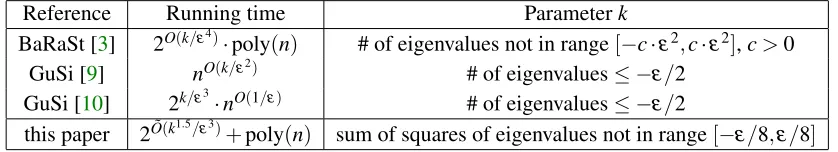
Reference Running time Parameterk

BaRaSt [3] 2O(k/ε4)_{·poly(n) # of eigenvalues not in range[−c·}

ε2,c·ε2],c>0 GuSi [9] nO(k/ε2) _{# of eigenvalues≤ −}

ε/2 GuSi [10] 2k/ε3_·nO(1/ε) _{# of eigenvalues≤ −ε/2}

this paper 2O(k˜ 1.5/ε3)_{+poly(n) sum of squares of eigenvalues not in range[−}

ε/8,ε/8]

Table 1: A comparison between previous algorithms applied to Max Cut and our algorithm.

Table 1gives a comparison between previous algorithms applied to Max Cut and our algorithm. Unlike the previous algorithms, our algorithm rounds the solution to a fixed size LP, as opposed to a SDP hierarchy. The advantages over previous algorithms, besides the simplicity of the algorithm, is a faster

1_{Throughout the paper we use ˜O(.)to denote that logarithmic terms are ignored.}

2_{The normalization one needs for dense graphs is different from what we use in this paper. IfGis a graph with average}

running time and the dependency on a potentially smaller threshold-rank parameter, because the running time of our algorithm depends on thesum of squaresof eigenvalues outside of a certain range, rather than the number of such eigenvalues. Recall that the eigenvalues ofD−1/2AD−1/2are in the range[−1,1].

We now give a precise statement of our results, after introducing some notation.

2

Statement of results

2.1 Notation

LetG= (V,E)be a (weighted) undirected graph withn:=|V|vertices. LetAbe the adjacency matrix of G. For any vertexu∈V, let

d(u):=

_∑

Au,v

be the degree ofu. For a set S⊂V, let the volume ofS be the summation of vertex degrees in S, d(S) =∑v∈Sd(v), and let

m:=d(V) =

_∑

d(v).

LetDbe the diagonal matrix of degrees. For any matrixM∈_RV×V_{, we use}

M_D:=D−1/2MD−1/2.

Observe that ifGis ad-regular graph, thenM_D=M/d. We callA_Dthenormalized adjacency matrixof G. It is straightforward to see that all eigenvalues ofA_Dare contained in the interval[−1,1].

For two functions f,g∈V →_R, lethf,gi:=∑v∈V f(v)g(v). Also, let f⊗gbe the tensor product of

f,g; i. e., the matrix inRV×V such that(u,v)entry is f(u)·g(v). For a function f∈RV, andS⊆V let

f(S):=∑v∈Sf(v).

For a setS⊆V, let1Sbe the indicator function ofS, and let

dS(v):=

(

d(v) v∈S,

0 otherwise.

For any two setsS,T ⊆V, andα∈R, we use the notation

CUT(S,T,α):=α·(dS⊗dT)

to denote the matrix corresponding to the cut(S,T), where(u,v)entry of the matrix isα·d(u)·d(v)if

u∈S,v∈T and zero otherwise. We remark that CUT(S,T,α)is not necessarily a symmetric matrix.

Definition 2.1(Matrix norms). For a matrixM∈_RV×V_{, andS,T ⊆V, let}

M(S,T):=

_∑

Mu,v.

The Frobenius norm and the cut norm are defined as follows:

kMk_F := r

_∑

M2

u,v,

kMk_C := max

Definition 2.2(Sum-of-squares threshold rank). For any unweighted graphG, with normalized adjacency matrixA_D, letλ1, . . . ,λnbe the eigenvalues ofADwith the corresponding eigenfunctions f1, . . . ,fn. For δ>0, theδ-sum-of-squares threshold rank ofAis defined as

t_δ(A_D):=

_∑

λi2.

Also, theδ-threshold approximation ofA_Dis defined as

T_δ(A_D):=

_∑

λifi⊗fi.

In words,T_δ(A_D)is an approximation ofA_Dobtained by removing the projection on eigenvectors corresponding to the small eigenvalues. It is well known thatT_δ(A_D)is the best approximation of its rank toA_Din`2and Frobenius norm. InLemma 3.1, below, we show thatD1/2Tδ(AD)D1

/2_{is always a good} approximation ofAincut norm.

2.2 Matrix decomposition theorem

The following matrix decomposition theorem is the main technical result of this paper.

Theorem 2.3. For any graph G, andε >0, let k:=t_ε/2(A_D). There is an algorithm that writes A as a linear combination of cut matrices, W(1),W(2), . . . ,W(σ), such thatσ≤16k/ε2, and

A−W

(1)_{− · · · −W}(σ)

C≤εm,

where each W(i)is a cut matrixCUT(S,T,α), for some S,T ⊆V , such that|α| ≤ √

k/m and m is the sum of the degrees of all vertices of G. The running time of the algorithm is polynomial in n,k,1/ε.

2.3 Algorithmic applications

Our main algorithmic application ofTheorem 2.3is the following theorem that approximates any cut on low threshold-rank graphs with a running time 2O(k˜ 1.5/ε3)_+poly(n).

Theorem 2.4. Let G= (V,E), and for a givenε>0, let k:=t_ε/8(AD). There is a randomized algorithm such that for either of maximum cut or minimum cut problems over sets of volume

Γ−εm/2≤ |S| ≤Γ+εm/2,

in time2O(k˜ 1.5/ε3)_+poly(n,k,1/

ε), with constant probability finds a set S such that|d(S)−Γ| ≤εm and

A(S,S)≥ max

Γ−εm/2≤|S∗_|≤Γ+εm/2A(S

∗_,

S∗)−εm

if it is a maximization problem, and

A(S,S)≤ min

Γ−εm/2≤|S∗_|≤Γ+εm/2A(S

∗_,S∗_{) +εm}

In the minimum bisection problem we want to find the smallest cut with equal volume in both sides of the cut,

min

S:d(S)=m/2

A(S,S).

Similarly, in the maximum bisection problem we want to find the maximum cut with equal volume in both sides. Although in the literature a bisection is typically defined as the cut with equal number of verticesin the both sides, here we study cuts with (approximately) equal volume in both sides. This is because of a limitation of spectral algorithms (cf. Cheeger’s inequality for finding the minimum bisection). Nonetheless, the applications are very similar (e. g., we can use above corollary in divide and conquer algorithms to partition a given graph into small pieces with few edges in between).

We use the above theorem to provide a PTAS for maximum cut, maximum bisection, and minimum bisection problems.

Corollary 2.5. Let G= (V,E), and for a givenε>0, let k:=t_ε/8(AD). There is a randomized algorithm that in time2O(k˜ 1.5/ε3)_{+poly(n,k,1/ε)finds anεm additive approximation of the maximum cut.}

Proof. We can simply guess the size of the optimum within an εm/2 additive error and then use

Theorem 2.4.

Corollary 2.6. Let G= (V,E), and for a givenε>0, let k:=t_ε/8(AD). For any of the maximum bisection and minimum bisection problems, there is a randomized algorithm that in time2O(k˜ 1.5/ε3)_{+poly(n,k,1/ε)}

finds a cut(S,S)such that|d(S)−m/2| ≤εm and that A(S,S)provides anεm additive approximation of

the optimum.

Proof. For the maximum/minimum bisection the optimum must have sizem/2. So we can simply use

Theorem 2.4withΓ=m/2.

3

Regularity lemma for low threshold-rank graphs

In this section we proveTheorem 2.3. The first step is to approximateAby a low-rank matrixB. In the next lemma we constructBsuch that the value of any cut inAis approximated within a small additive error inB.

Lemma 3.1. Let A be the adjacency matrix of G. For0≤δ <1, let

B:=D1/2T_δ(A_D)D1/2.

Then,kA−Bk_C≤δm.

f1, . . . ,fn. For anyS,T ⊆V, we have

h1S,(A−B)1Ti = hD1/21S,(A−B)DD1/21Ti

= hpdS,(A_D−T_δ(A_D))pdTi

≤ δ·

_∑

hpdS,fiih

p dT,fii

≤ δ·

s

∑

hpdS,fii2·

s

∑

hpdT,fii2

≤ δ·

p dS

·

p dT

≤δ·

p dV

2

=δm,

where the second inequality follows by the Cauchy–Schwarz inequality. The lemma follows by noting the fact thatkA−Bk_Cis the maximum of the above expression for anyS,T ⊆V.

By the above lemma if we approximateBby a linear combination of cut matrices, then it is also a good approximation ofA. Moreover, sincet_δ(A_D) =t_δ(B_D),Bhas a small sum-of-squares threshold rank iffAhas a small sum-of-squares threshold rank.

Lemma 3.2. For any graph G with adjacency matrix A,δ >0, and B=D1/2T_δ(A_D)D1/2,

kB_Dk2_F =t_δ(A_D).

Proof. The lemma follows from the fact that the square of the Frobenius norm of any matrix is equal to the summation of square of eigenvalues. Ifλ1, . . . ,λnare the eigenvalues ofAD, then

kB_Dk2_F=trace(B_D2) =

_∑

|λi|>δ

λi2=tδ(AD).

Note that in the first equality we are using the fact thatB_Dis a symmetric matrix.

The next proposition is the main technical part of the proof ofTheorem 2.3. We show that we can write any (not necessarily symmetric) matrixBas a linear combination ofO(kBk2_F/ε2)cut matrices such that the cut norm ofBis preserved within an additive error ofεm. The proof builds on the existential theorem of Frieze and Kannan [7, Theorem 7].

Proposition 3.3. For any matrix B∈RV×V, k=kBDk2F, andε>0, there exist cut matrices

W(1),W(2), . . . ,W(σ),

such thatσ≤1/ε2, and for all S,T ⊆V ,

B−W(1)−W(2)− · · · −W(σ)

(S,T)

≤ε

p

k·d(S)·d(T),

Proof. LetR(0)=B. We use the potential functionh(R):=kR_Dk2_F. We show that as long as there are S,T ⊆V such that

|R(S,T)|>εpkd(S)d(T)

we can add new cut matrices iteratively while maintaining the invariant that each time the value of the potential function decreases by at leastε2h(B). Sinceh(R(0)) =h(B), after at most 1/ε2we obtain a good approximation ofB.

Assume that afteri<1/ε2iterations,R(i)=B−W(1)− · · · −W(i). Suppose for someS,T ⊆V,

R

(i)_(S,T) >ε·

p

h(B)·d(S)·d(T) =ε·pk·d(S)·d(T). (3.1)

ChooseW(i+1)=CUT(S,T,α), for

α = R

(i)_(S,T)

d(S)·d(T),

and letR(i+1)=R(i)−W(i+1). Note that for any pair of verticesu,v∈V ifu∈/Sorv∈/T, thenR(i+u,v1)=

R(i)u,v. So,

h(R(i+1))−h(R(i)) =

_∑

(R(i)u,v−αd(u)d(v))2−R(i)u,v

2

d(u)d(v)

= −2αR(i)(S,T) +α2d(S)d(T)

= −R

(i)_(S,T)2

d(S)d(T) ≤ −ε

2_·h(B).

The last equality follows by the definition of α, and the last inequality follows from Equation (3.1). Therefore, after at mostσ≤1/ε2iterations, (3.1) cannot hold for allS,T⊆V.

Although the previous proposition only proves the existence of a decomposition into cut matrices, we can construct such a decomposition efficiently using the following nice result of Alon and Naor [1] that gives a constant factor approximation algorithm for the cut norm of any matrix.

Theorem 3.4(Alon and Naor [1]). There is a polynomial time randomized algorithm such that for any given A∈RV×V, with high probability, finds sets S,T ⊆V , such that

|A(S,T)| ≥0.56kAk_C.

Now we are ready to proveTheorem 2.3.

Proof ofTheorem 2.3. Letδ :=ε/2, andB:=D1/2Tδ(AD)D1/2. ByTheorem 3.1, we have that

kA−Bk_C≤δm=εm/2. (3.2)

So we just need to approximateBby a set of cut matrices within an additive error ofεm/2. For a matrix

Letε0:=ε/ √

4k. We use the proof strategy ofProposition 3.3. LetR(i)=B−W(1)− · · · −W(i). If

R(i)

C≥ε

0√_{km, then byTheorem 3.4in polynomial time we can findS,T ⊆V such that}

R

(i)_(S,T) ≥ε

0_·√

k·m/2≥ε0·

p

h(B)·m/2. (3.3)

ChooseW(i+1)=CUT(S,T,α), forα=R(i)(S,T)/m2, and letR(i+1)=R(i)−W(i+1). We get

h(R(i+1))−h(R(i)) =−2αR(i)(S,T) +α2d(S)d(T)≤ −R

(i)_(S,T)2

m2 ≤ −

ε02·h(B)

4 .

Sinceh(R(0)) =h(B), afterσ≤4/ε02=16k/ε2, we haveR(σ)

C≤ε

0√_{km. Using the triangle inequality}

on the cut norm we obtain

A−W

(1)_{− · · · −W}(σ)

C ≤ kA−B k_C+

B−W

(1)_{− · · · −W}(σ)

C ≤ εm/2+ε0

√

km=εm.

where the second inequality uses (3.2).

This proves the correctness of the algorithm. It remains to upper boundα. For each cut matrix

W(i)=CUT(S,T,α)constructed throughout the algorithm we have

|α|=|R

(i)_(S,T)|

m2 =

1 m2

∑

R(i)u,v

p

d(u)d(v)

p

d(u)d(v)

≤ 1 m2 v u u t

_∑

u∈S,v∈T

R(i)u,v

2

d(u)d(v)

p

d(S)d(T)

≤ 1 m v u u t

∑

R(i)u,v

2

d(u)d(v)

=

p h(R(i)₎

m ≤

p h(B)

m =

√

k m .

where the first inequality follows by the Cauchy–Schwarz inequality, the second inequality usesd(S),d(T)≤

m, and the last inequality follows by the fact that the potential function is decreasing throughout the algorithm. This completes the proof of theorem.

4

Fast approximation algorithm for low threshold-rank graphs

In this section we proveTheorem 2.4. First, byTheorem 2.3in time poly(n,k,1/ε)we can find cut matricesW(1), . . . ,W(σ)forσ=O(k/ε2), such that for all 1≤i≤t,W(i)=CUT(Si,Ti,αi),αi≤

√

k/m, and

whereW:=W(1)+· · ·+W(σ). It follows from the above equation that for any setS⊆V,

|A(S,S)−W(S,S)|=

A(S,S)−

σ

∑

αi·d(S∩Si)·d(S∩Ti)

≤

εm

4 . (4.1)

Fix S∗⊆V of volume Γ−ε/2≤d(S∗)≤Γ+ε/2 (think of (S∗,S∗) as the optimum cut), and let s_i∗:=d(Si∩S∗), andti∗:=d(Ti∩S∗). Observe that by Equation (4.1),

A(S∗,S∗)− σ

∑

αis∗it

∗

i

≤εm

4 . (4.2)

Letαmax:=max1≤i≤σ|αi|. Choose∆=Θ(ε3m/k1.5)such that

∆≤min

n_ε3·m 48 ,

ε 48αmax·σ

o

. (4.3)

Note that this is achievable sincek≥1,αmax≤

√

k/mandσ =O(k/ε2).

We define an approximation ofs∗_i,t_i∗by rounding them down to the nearest multiple of∆, i. e.,

˜

s∗_i :=∆· bs∗i/∆c,

˜

t_i∗:=∆· bti∗/∆c.

We use ˜s∗,t˜∗ to denote the vectors of the approximate values. It follows that we can obtain a good approximation of the size of the cut(S∗,S∗_{)just by guessing the vectors ˜s}∗_{and ˜t}∗_{. Since|s}∗

i −s˜∗i| ≤∆

and|t_i∗−t˜_i∗| ≤∆, we get

σ

∑

|s∗_it_i∗αi−s˜i∗t˜i∗αi| ≤σ·αmax(2·∆·m+∆2)≤3αmax·σ·∆·m≤ε·m/16, (4.4)

where we used (4.3).

Observe that by Equations (4.1), (4.2), and (4.4), if we know the vectors ˜s∗,t˜∗, then we can find A(S∗,S∗)within an additive error ofεm/2. Since ˜s_i∗,t˜_i∗≤m, there are onlyO(m/∆)possibilities for each

˜

s∗_i and ˜t_i∗. Therefore, we afford to enumerate all possible values of them in time(m/∆)2σ, and choose the

one that gives the largest cut. Unfortunately, for a given assignment of ˜s∗,t˜∗the corresponding cut(S∗,S∗)

may not exist. Next we give an algorithm that for a given assignment of ˜s∗,t˜∗finds a cut(S,S)such that

A(S,S) =

_∑

˜

s∗_it˜_i∗αi±εm,

if one exists.

First we distinguish the large degree vertices ofGand simply guess which side they are mapped to in the optimum cut. For the rest of the vertices we use the solution of LP(1). Let

be the set of large degree vertices. Observe that|U| ≤m/∆. LetPbe the coarsest partition of the set

V\Usuch that for any 1≤i≤σ, bothSi\U andTi\Ucan be written as a union of sets inP, and for

eachP∈P,d(P)≤∆. Observe that|P| ≤22σ+m/∆. For a given assignment of ˜s∗,t˜∗, first we guess the

set of vertices inUthat are contained inS∗,US∗ :=S∗∩U, andUS∗:=U\US∗. For the rest of the vertices

we use the linear program LP(1) to find the unknownd(S∗∩P).

LP(1)

0 ≤ yP ≤ 1 ∀P∈P

Γ−εm/2 ≤

_∑

yPd(P) +d(US∗) ≤ _Γ+_εm/2 (4.5)

˜

s∗_i ≤

_∑

P⊆Si

yPd(P) +d(US∗∩S_i) ≤ s˜∗_i +_∆ ∀1≤i≤_σ (4.6)

˜

t_i∗ ≤

_∑

P⊆Ti

(1−yP)d(P) +d(U_S∗∩Ti) ≤ t˜i∗+∆ ∀1≤i≤σ. (4.7)

Observe thatyP=d(S∗∩P)/d(P)is a feasible solution to the linear program. In the next lemma which is

the main technical part of the analysis we show how to construct a set based on a given solution of the LP.

Lemma 4.1. There is a randomized algorithm such that for any S∗⊂V , givens˜∗_i,t˜_i∗and US∗ returns a random set S such that

P

W(S,S)≥A(S∗,S∗)−3εm

4 ∧ |d(S)−Γ| ≤εm

≥ ε

4, (4.8)

P

W(S,S)≤A(S∗,S∗_{) +}3εm

4 ∧ |d(S)−Γ| ≤εm

≥ ε

4. (4.9)

Proof. Letybe a feasible solution of LP(1). We use a simple independent rounding scheme to compute arandomsetS. We always includeUS∗ inS. For eachP∈P, we includePinS, independently, with probabilityyP. We prove thatSsatisfies the lemma’s statements.

First of all, by linearity of expectation,

E[d(S∩Si)] =d(US∗) +

_∑

P⊆Si

yPd(P), and

Ed(S∩Ti)

=d(U_S∗) +

∑

P⊆Ti

(1−yP)d(P).

Therefore, by (4.5),

|E[d(S)]−Γ| ≤εm/2. (4.10)

Furthermore, by (4.6) and (4.7) for any 1≤i≤σ,

|E[S∩Si]−s˜∗i| ≤∆ and |E

S∩Ti

−t˜_i∗| ≤∆. (4.11)

Claim 4.2. P[|d(S)−Γ| ≥εm]≤ ε 12.

Proof. We use the theorem of Hoeffding to prove the claim:

Theorem 4.3(Hoeffding Inequality). Let X1, . . . ,Xnbe independent random variables such that for each

1≤i≤n, Xi∈[0,ai]. Let X:=∑ni=1Xi. Then, for anyε>0

P[|X−E[X]| ≥ε]≤2 exp

− 2ε

2

∑ni=1a2i

.

Now, by the independent rounding procedure, we obtain

P[|d(S)−E[d(S)]| ≥εm/2]≤2 exp

− ε

2_m2

2∑Pd(P)2

≤ 2 exp

−ε

2_m2

2m∆

≤ 2 exp(−24/ε)≤ ε 12,

where the second inequality follows by the fact thatd(P)≤∆and∑Pd(P)≤mand the third inequality

follows by (4.3). The claim flows by (4.10).

In the next claim we upper bound the expected value ofW(S,S)−A(S∗,S∗).

Claim 4.4. E

W(S,S)

−A(S∗,S∗)≤

εm 2 .

Proof. First, we calculateEW(S,S)in terms ofE[d(S∩Si)],Ed(S∩Ti)

.

EW(S,S)=E

"

σ

∑

d(S∩Si)d(S∩Ti)αi

#

= σ

∑

αiE

"

∑

d(P)I[P⊆S]

!

∑

d(Q)IQ⊆S

!# + σ

∑

d(US∗∩Si)Ed(S∩Ti)

+d(U_S∗∩Ti)E[d(S∩Si)]

.

(4.12)

Since the event thatP⊆Sis independent ofQ⊆S, iffP6=Qwe get

EI[P⊆S]IQ⊆S=

(

yP(1−yQ) ifP6=Q,

0 otherwise.

Letsi:=E[d(S∩Si)]andti:=Ed(S∩Ti)

. By (4.12) and the above equation,

EW(S,S) =

σ

∑

αisiti− σ

∑

αi

∑

Using Equation (4.2) we write

E

W(S,S)−A(S∗,S∗)

≤ E

W(S,S)− σ

∑

αis∗it

∗ i + εm 4 = σ

∑

(αisiti−αis∗it

∗

i)− σ

∑

∑

αiyP(1−yP)d(P)2

+ εm 4 ≤ σ

∑

|αisiti−αis˜∗it˜

∗

i|+ σ

∑

|αis˜∗it˜

∗

i −αis∗it

∗

i|+σ αmaxm∆+εm

4

≤ σ

∑

|αisiti−αis˜∗it˜i∗|+ εm 16 + εm 48 + εm 4 ≤ εm 2 ,

where the equality follows by (4.13), the second inequality follows by the fact thatd(P)≤∆for allP∈P

and∑Pd(P)≤m, the third inequality follows by (4.4) and (4.3), and the last equation can be proved

similar to (4.4) using (4.11). This completes the proof ofClaim 4.4.

Now, we are ready finish the proof ofLemma 4.1. Here, we prove (4.8). Equation (4.9) can be proved similarly. ByClaim 4.4,

EW(S,S)≥A(S∗,S∗)−ε

m 2 .

Since the size of any cut inGis at mostm/2, by (4.1), for anyS⊆V,W(S,S)≤εm/4+m/2<3m/4. Therefore, by Markov’s inequality,

P

W(S,S)≥A(S∗,S∗)−3εm

4

≥ε

3.

By the union bound,Lemma 4.1follows from the discussion above andClaim 4.2.

Our rounding algorithm is described inAlgorithm 1. First, we prove the correctness, then we calculate the running time of the algorithm. LetSbe the output set of the algorithm. First, observe that the output always satisfies|d(S)−Γ| ≤εm. Now letA(S∗,S∗)be the maximum cut among all sets of sizeΓ(the

minimization case can be proved similarly). In the iteration that the algorithm correctly guesses ˜s∗_i,t˜_i∗,US∗, there exists a feasible solutionyof LP(1). byLemma 4.1, for all 1≤i≤4/ε,

P

W(Sy(i),Sy(i))≥A(S∗,S∗)−

3εm

4 ∧ |d(Sy(i))−Γ| ≤εm

≥ε

4.

Since we take the best of 4/ε samples, with probability 1/ethe output setSsatisfies

W(S,S)≥A(S∗,S∗_)−3εm/4.

Algorithm 1Approximate Maximum Cut(S,S)such thatd(S) =Γ±εm

for allpossible values of ˜s∗_i,t˜_i∗, andUS∗⊆U do ifthere is a feasible solutionyof LP(1)then

fori=1→4/εdo

Sy(i)←US∗.

For eachP∈PincludePinSy(i), independently, with probabilityyP.

end for end if end for

return among all sets Sy(i) sampled in the loop that satisfy |d(Sy(i))−Γ| ≤ εm, the one that

W(Sy(i),Sy(i))is the maximum.

LP(1). Since the size of LP is 2O(k˜ /ε2)_{, in this caseAlgorithm 1terminates in time 2}O(k˜ /ε2)_{. Note that for}

any sample setSy(i), bothd(Sy(i))andW(Sy(i),Sy(i))can be computed in time 2O(k˜ /ε

2₎

, once we know

|Sy(i)∩P|for anyP∈P.

Otherwise if|U| k/ε2, the dependence of the running time of the algorithm onε,kis dominated by the step where we guess the subset ofUS∗=U∩S∗. By (4.3),

|U| ≤m

∆ =O

k1.5

ε3

.

Therefore,Algorithm 1runs in time 2O(k˜ 1.5/ε3)_{. Since it takes poly(n,k,1/ε)to compute the decomposition}

intoW(1), . . . ,W(σ), the total running time is 2O(k˜ 1.5/ε3)_{+poly(n,k,1/ε). This completes the proof of} Theorem 2.4.

Acknowledgement.

We would like to thank an anonymous reviewer for helpful comments.

References

[1] NOGA ALON AND ASSAF NAOR: Approximating the cut-norm via Grothendieck’s in-equality. SIAM J. Comput., 35(4):787–803, 2006. Preliminary version in STOC’04. [doi:10.1137/S0097539704441629] 248

[2] SANJEEVARORA, BOAZBARAK,ANDDAVIDSTEURER: Subexponential algorithms for Unique

Games and related problems. InProc. 51st FOCS, pp. 563–572. IEEE Comp. Soc. Press, 2010. [doi:10.1109/FOCS.2010.59] 242

[3] BOAZBARAK, PRASADRAGHAVENDRA, ANDDAVIDSTEURER: Rounding semidefinite

[4] AMIN COJA-OGHLAN, COLINCOOPER,ANDALANM. FRIEZE: An efficient sparse regularity concept. SIAM J. Discrete Math., 23(4):2000–2034, 2010. Preliminary version in SODA’09. [doi:10.1137/080730160] 243

[5] WENCESLASFERNANDEZ DE LAVEGA, MAREKKARPINSKI, RAVIKANNAN,ANDSANTOSH

VEMPALA: Tensor decomposition and approximation schemes for constraint satisfaction problems. InProc. 37th STOC, pp. 747–754. ACM Press, 2005. [doi:10.1145/1060590.1060701] 243

[6] ALAN M. FRIEZE AND RAVI KANNAN: The regularity lemma and approximation schemes for dense problems. In Proc. 37th FOCS, pp. 12–20. IEEE Comp. Soc. Press, 1996. [doi:10.1109/SFCS.1996.548459] 242

[7] ALAN M. FRIEZE AND RAVI KANNAN: Quick approximation to matrices and applications. Combinatorica, 19(2):175–220, 1999. [doi:10.1007/s004930050052] 242,247

[8] MICHELX. GOEMANS ANDDAVID P. WILLIAMSON: Improved approximation algorithms for maximum cut and satisfiability problems using semidefinite programming. J. ACM, 42(6):1115– 1145, 1995. Preliminary version inSTOC’94. [doi:10.1145/227683.227684] 242

[9] VENKATESAN GURUSWAMI ANDALI KEMAL SINOP: Lasserre hierarchy, higher eigenvalues, and approximation schemes for graph partitioning and quadratic integer programming with PSD objectives. InProc. 52nd FOCS, pp. 482–491. IEEE Comp. Soc. Press, 2011. Expanded version in

CoRR (2011). Merged with [11] inCoRR (2013). [doi:10.1109/FOCS.2011.36] 242,243,255

[10] VENKATESAN GURUSWAMI AND ALI KEMAL SINOP: Faster SDP hierarchy solvers for local rounding algorithms. InProc. 53rd FOCS, pp. 197–206. IEEE Comp. Soc. Press, 2012. Expanded version inCoRR. [doi:10.1109/FOCS.2012.58] 242,243

[11] VENKATESANGURUSWAMI ANDALIKEMALSINOP: Approximating non-uniform sparsest cut via generalized spectra. InProc. 24th Ann. ACM-SIAM Symp. on Discrete Algorithms (SODA’13). SIAM, 2013. Expanded version, merged with [9] inCoRR (2013). [doi:10.1137/1.9781611973105.22]

242,255

[12] ALEXANDRAKOLLA: Spectral algorithms for Unique Games.Comput. Complexity, 20(2):177–206, 2011. Preliminary versions inCCC’10andECCC (2010). [doi:10.1007/s00037-011-0011-7] 242

[13] ALEXANDRA KOLLA AND MADHUR TULSIANI: Playing Unique Games using graph spectra.

manuscript, 2007. 242

[14] JEAN B. LASSERRE: Global optimization with polynomials and the problem of moments. SIAM J. Optim., 11(3):796–817, 2001. [doi:10.1137/S1052623400366802] 242

[16] PABLOA. PARRILO:Structured semidefinite programs and semialgebraic geometry methods in robustness and optimization. Ph. D. thesis, California Institute of Technology, 2000. 242

[17] ENDRESZEMERÉDI: Regular partitions of graphs. Colloq. Internat. CNRS: Problèmes Combina-toires et Théorie des Graphes, 260:399–401, 1978.242

AUTHORS

Shayan Oveis Gharan Assistant Professor

University of Washington, Seattle, WA shayan cs washington edu

http://homes.cs.washington.edu/~shayan

Luca Trevisan Professor

U.C. Berkeley, Berkeley, CA luca berkeley edu

http://www.cs.berkeley.edu/~luca/

ABOUT THE AUTHORS

SHAYANOVEISGHARAN(listed alphabetically under “O”) is an assistant professor in the Computer Science and Engineering departmentat theUniversity of Washington. He received his Ph. D. in 2013 from theMS&E departmentatStanford Universityunder the supervision ofAmin SaberiandLuca Trevisan. Before joining UW he spent a year and a half as a postdoctoralMiller Fellowat UC Berkeley where his host wasUmesh Vazirani. He did his undergraduate studies at the Computer Engineering department at

Sharif University. Shayan’s research areas include the design and analysis of algorithms, spectral graph theory and applied probability. Shayan received an ACM doctoral dis-sertation award honorable mention for his Ph. D. thesis “New Rounding Techniques for the Design and Analysis of Approximation Algorithms” in 2014. He and his coauthors received the Best Paper awards at SODA 2010 and FOCS 2011 for their work on the Traveling Salesman Problem.