Dynamic Nonuniform Data Approximation in
Databases with Haar Wavelet
Su Chen
Dept. of Computer Science, Rutgers University, Piscataway, NJ, USA [email protected]
Antonio Nucci
Narus Inc., Mountain View, CA, USA [email protected]
Abstract— Data synopsis is a lossy compressed represen-tation of data stored into databases that helps the query optimizer to speed up the query process, e.g. time to retrieve the data from the database. An efficient data synopsis must provide accurate information about the distribution of data to the query optimizer at any point in time. Due to the fact that some data will be queried more often than others, a good data synopsis should consider the use of nonuniform accuracy, e.g. provide better approximation of data that are queried the most. Although, the generation of data synopsis is a critical step to achieve a good approximation of the initial data representation, data synopsis must be updated over time when dealing with time varying data. In this paper, we introduce new Haar wavelet synopses for nonuniform accuracy and time-varying data that can be generated in linear time and space, and updated in sublinear time. We further introduce two linear algorithms, called 2-Step and M-Step for the Point-wise approximation problem that clearly outperforms previous algorithms known in literature, and two new algorithm called,Data Mapping and Weight Mapping for theRange-sum approximation problem that, to the best of our knowledge, represent a key research milestone as being the first linear algorithm for arbitrary weights. For both scenarios, we focus not only on the generation of the data synopsis but also on their updates over time. The efficiency of our new data synopses is validated against other linear methods by using both synthetic and real data sets.
Index Terms— Dynamic data synopsis, query optimization, nonuniform lossy compression, point-wise and range-sum approximation, linear complexity
I. INTRODUCTION
How to efficiently query data is a fundamental problem in databases. Estimating the cost of complex queries, reflecting CPU time, memory usage and I/O operations, requires a detailed knowledge of how data are distributed and stored into database tables. In practice, any database system maintains a concise lossy compressed data struc-ture, called data synopsis, that approximates the data distribution at any point in time. The query optimizer will use this data summary to decide how a query is executed in order to retrieve the requested data at the minimal cost in terms of overall processing overhead. Besides accuracy, the cost of generating and updating synopses is a major This paper is based on “Nonuniform Compression in Databases with Haar Wavelet”, by S. Chen and A. Nucci, which appeared in the Proceedings of IEEE Data Compression Conference(DCC), pp. 223-232, Snowbird, USA, March 2007 c2007 IEEE.
concern, since the cost of optimization may overwhelm its benefits if the cost of synopsis is too large.
According to the characteristics of the environment at which data synopses are applied, data synopses might be classified as (i) Uniform vs. Nonuniform and (ii) Static vs. Dynamic.
Data synopses applied to data that require the same quality of approximation are known as “uniform”. All data subset will be represented by the same weight, that reflects the fact that any data subset must be treated in the exact same way as the others. Scenarios in which at least one data subset is required to be known with a better quality of approximation than others, e.g. for example because it might be invoked in the query process more often than the others, are known as “nonuniform”. In this case, the weight associated to each data subset will be different; the larger is the value of its weight the higher is the quality of its approximation for the data subset.
At the same time, data synopses can be defined for “static” or “dynamic” data structures. When data and weights do not change over time, it is said to be “static”. In this context, it is important to generate a good data synopsis for the data on hands. When data or weights change over time, the scenario is said to be “dynamic”. Dynamic scenarios are challenging to be managed. In this case, data synopses should be well generated and updated over time in order to provide approximated answers with high accuracy and thus provide meaningful information to the query optimizer at any point in time.
There are two types of data synopses that can be used to answer database queries: Point-wise approximation and
Range-sum approximation. The Point-wise approximation
is defined for single data point query while the Range-sum approximation is defined for data intervals query, e.g. set of data points. As a consequence, Point-wise approximation can be seen as a special case of Range-sum approximation when the data interval collapses into one single data point.
In this paper, we introduce new wavelet data synopses that can be generated in linear time and updated in sublinear time for dynamic-data and nonuniform weights. Our major contributions are summarized in the following.
First, we propose two linear algorithms for the Point-wise
clearly show how the proposed algorithms outperform weighted wavelet algorithm [1] on approximation error on both synthetic and real data sets with only O(B3) extra running time, whereBrepresents the approximation space. Second, we propose two linear algorithms for the Range-sum approximation problem called Data-mapping and Weight-mapping. To the best of our knowledge, these algorithms represent the first linear algorithms ever proposed in literature for arbitrary weights. Fornweights and B compression space, we show that both time and space complexity is O(n2 +B3), which is linear to the weight size O(n2). Third, all the algorithms we proposed in this paper are the first ones that focus not only on the generation of the data synopsis but also on its updates overtime. For dynamic data and weights, the time complexity of synopsis updates isO(log(n)+B3)for point-wise approximation andO(n+B3)for range-sum approximation. Fourth, we show that when the structure of given weights can be simplified, our algorithm can be tuned accordingly, and the complexity for range-sum synopses generation can be reduced fromO(n2+B3)to
O(n+B3).
The remainder of this paper is structured as following. Section II provides the mathematical definition of Point-wise and Range-sum approximations and introduces the related work. In Sections III and IV we present two new algorithms for generating Point-wise approximation, e.g. 2-step and M-step, and two new algorithms for generating Range-sum approximation, e.g. Data-mapping and Weight-mapping. In section V, we introduce the novel incremental method that can minimize the computational cost when experiencing dynamic data and weights. In sec-tion VI we introduce three examples where our algorithm can simplify the inner states, which is used to accelerate the synopses generation, if the weights have patterns inside. As a result, the overall cost can be reduced to sublinear in term of the input weight size. In Section VII we validate the performance achieved by these algorithms using both synthetic and real-data, while Section VIII concludes the paper.
II. PROBLEMSTATEMENT ANDPREVIOUS WORK Small space synopses in database systems have been studied over decades to improve both the accuracy and the efficiency of the query approximation and query optimization. Traditional data synopses only represent the data that reside in the database, but they lack of considering the characteristic of the data being queried. As a consequence, data queried more often than others are treated exactly in the same way and thus the overall quality of the approximations produced ends to be poor.
Query Feedback systems [2]–[7] have been proposed
to address this problem. In these systems, data approxi-mations are corrected by their real values returned from queries, so that the frequently visited data can be more accurate than the others. An example of such feedback mechanism is represented by systems like LEO [7]. However query workload information is not fully explored
D[2] D[1] D[0]
D[4] D[5]
D[3]
D[6] D[7]
0=(1, 1, 1, 1, 1, 1, 1, 1)/(22) 1=(1, 1, 1, 1,-1,-1,-1,-1)/(22) 2=(1, 1,-1,-1, 0, 0, 0, 0)/2 3=(0, 0, 0, 0, 1, 1,-1,-1)/2 4=(1,-1, 0, 0, 0, 0, 0, 0)/2 5=(0, 0, 1,-1, 0, 0, 0, 0)/2 6=(0, 0, 0, 0, 1,-1, 0, 0)/2 7=(0, 0, 0, 0, 0, 0, 1,-1)/2
Figure 1. Wavelet transform of signal A
in these systems, since the data accuracy only reflect how recently the data is queried, but not how often the data is queried.
Only recently, real weights that indicate the frequency of data being queried are extracted from workloads and used to generate “usage-oriented” synopses [1], [8], [9]. In this paper, we use weights from workloads instead of query feedback mechanism to quantify the accuracy of our data synopses.
Considerable work is available in literature for the Point-wise data synopses generation when using his-togram data synopses [2], [3], [8], [10]–[12]. However, most recently, several papers [1], [13]–[17] remark the effectiveness of using wavelet decomposition in reducing large amount of data to compact sets of wavelet coeffi-cients, termed wavelet synopses. Wavelet synopses have been proved to provide fast and reasonably accurate ap-proximate answers to queries. Among wavelet synopses, the Haar wavelet synopsis has been found to be the most interesting one to be used in database due to its simple structure.
In this paper we focus on Haar wavelet synopsis applied to dynamic data and nonuniform weights for both Point-wise and Range-sum approximations. In figure 1, we show an example of wavelet transform of a signal A with length 8. The coefficients D are the inner product of the signal A, represented as ⊗, and the wavelet vectors
Ψ ={Ψ1, ...,Ψn}at different level, e.g.,D[i] =A⊗Ψi.
In the following we provide the mathematical definition of the two problems.
Problem 1 (Point-wise Approximation): LetA1×nbe a
generic data vector of dimension n and Π1×n be the weight vector of dimensionnthat reflects the approxima-tion quality of each data point ofA, e.g. to eachA[i]is associated a weightΠ[i]. The weight vector is normalized between [0,1], e.g. Pni=1Π[i] = 1. LetΨ be the set of
n candidate wavelets and B be the allowed number of wavelets to be used for the data synopsis. LetD be the set of coefficients associated to the B chosen wavelets, e.g.D[i]is associated to Ψi.
The Point-wise approximation problem can be stated as to identify the optimal subset of B wavelets from Ψ and their associated coefficientsD, in order to minimize the weighted Point-wise approximation error defined as:
ǫ(P)(A) =Xn
i=1
whereAbrepresents the wavelet approximation of data set
A, e.g.Ab=PBi=1D[i]Ψi
Problem 2 (Range-sum Approximation): Let A1×n be
a generic data vector of dimension n, and let A(i, j) =
Pj
k=iA[k], withi≤j, represent an additive function that
operates on all elements of data vector A from A[i] to
A[j]. LetΠn×nbe the weight matrix of dimensionn×n such thatΠ[i, j] = 0,∀i≥j. Each elementΠ[i, j] repre-sents the weight associated to A(i,j). The weight matrixΠ is normalized between[0,1], e.g.Pni=1Pnj=1Π[i, j] = 1. The Range-sum approximation problem can be stated as to identify the optimal subset of B wavelets fromΨ and their associated coefficientsD, in order to minimize the weighted Range-sum approximation error defined as:
ǫ(R)(A) =Xn
i=1
n X
j=1
Π[i, j](A(i, j)−Ab(i, j))2 (2)
where Ab(i, j) represents a generic linear function of the wavelet approximation of A(i, j), e.g. Ab(i, j) =
f(PBi=1D[i]Ψi).
Most of the wavelet synopses are generated under the assumption of uniform weights for both Point-wise and Range-sum approximations [13] [14] [15]. For Point-wise approximation, the Parseval’s theorem provides a solution that applies to all orthonormal data transforms, i.e., the best approximation is achieved by largest coefficients. For range-sum approximation, [15] presents an optimal solution on Haar wavelet synopsis.
The methods that study the more general case of nonuniform weights scenario result to be either sub-optimal in terms of approximation errors [1] or too expensive in terms of running time [18]. Matias and Urieli in [1] provided the first linear algorithm, called
Weighted-wavelet (W-wav), able to preserve Parseval’s
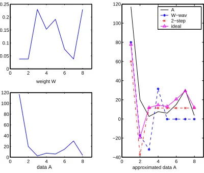
orthonormal condition by using a smart combination of wavelets and weights. As a result, their method provides the best synopses on weighted Haar bases, when choos-ing the largest coefficients as synopses. Unfortunately, this approach provides approximation errors that do not decrease monotonically with respect to the compression space B and the outcome approximation error may not be bounded. In Figure 2 we show with an example of what just stated. DataAis extracted from an exponential distribution. We define approximation error with B = 0 as ǫ0 = PiΠ[i]A[i]2, i.e. assume all data values are
0. The approximation error of W-wav with B = 0 is
ǫ0 = 623.49. With more compression spaceB = 2, the
error increases to686.55. Their approximation is far from the ideal approximation (see Section III), and worse than our 2-step method (see Section III) that reduces the error to 306.95 with B = 2. This problem exists not only for exponential data sets, but for all data sets that are characterized by only a few very large values.
Guha and Harb in [18] studied this problem for differ-entLpnorm errors. They proved that the best coefficients can be found by searching a bounded region that is specified by the optimal error of L∞. Because the real value of this optimal error is unknown, the algorithm
0 2 4 6 8
0 0.05 0.1 0.15 0.2 0.25
weight W
0 2 4 6 8
0 20 40 60 80 100 120
data A
0 2 4 6 8
−40 −20 0 20 40 60 80 100 120
approximated data A A W−wav 2−step ideal
Figure 2. W-wav algorithm is not optimal
needs to guess a value to run. The accuracy of the solution is strictly related to the cardinality of the search space. The larger the search space is, the more accurate the result will be at the cost of a higher running time. The time complexity reaches O(n3) for L2 error, and the space complexity is super linear to n. As a consequence, the complexity of their approach results to be too high for synopses used for databases.
In [9], the author studied a special case of this problem where the weights are assumed to be organized into k intervals, and a unique weight value is associated to each interval. The running time isO(nkB2log(n)). When
k=n, this case collapses to the Point-wise approximation problem, with a quadratic running timeO(n2B2)in terms ofn.
Conversely, data synopses generation for the more gen-eral case of range-sum approximation has received only little attention from the research community. Most of the work in literature has studied this problem in the context of uniform weights or hierarchical weights [10], [11], [19] ignoring completely the importance of the non-uniform workload scenario. In this paper, we extensively study this problem as well and propose two linear algorithms to generate range-sum synopses in the context of arbitrary weights.
We conclude this section by highlighting the fact that all previous work, for both point-wise and range-sum approximation has been focused only on the generation of the data synopses, but ignored the importance of a more realistic scenario in which both data and weights can change over time and thus the mechanism on how to update the data synopsis over time. We consider this case as well in the paper.
III. NONUNIFORM POINT-WISE APPROXIMATION PROBLEM
In order to approach this problem, let us define three variables that come to play into the problem (see Fig-ure 3): (i) the data vector A, (ii) the wavelet vectors
A ππππ wavelet vector
uniform weight case
weighted wavelet transform method
2-step method
Figure 3. Methods
order to generate data synopses. For nonuniform weights, the mapping is arbitrary. The W-wav algorithm combines the weight vector with the wavelet vector by stretching wavelets vertically. The new wavelet basis is thus weight-specific. Data synopsis obtained when considering a spe-cific weight vector might be sub-optimal for a different weight vector. As a result, the wavelet basis has to be recomputed every time a weight change is experienced, leading to large cost in database management. A different approach to solve this problem is to combine the weight vector with the data vector. The intuition behind this approach comes from a good understanding of the error function.
Given the data vector Aand the weight vectorΠ, the error function (Equation 1) can be formulated as:
ǫ(P)(A) = Xn
i=1
(pΠ[i]A[i]−pΠ[i]Ab[i])2
= Xn
i=1
(AW[i]−AbW[i])2 (3)
where Ab represents the approximation of A, while
AW[i] =pΠ[i]A[i].
With this simple manipulation, the error function has been reduced to a uniform-weight case. As a result, the best approximationAb∗ ofA can be solved fromAb∗[i] =
b
A∗
W[i]/
p
Π[i], where the optimal approximationAb∗W of
AW exists according to Parseval’s theorem. We refer to this method as ideal approximation. Unfortunately this method is impractical because it requires the knowledge of the weight value Π[i] for each point, and thus inad-missible because the compression space B is not large enough to store Π. One might consider to introduce an approximation of Π but this will lead to a strong sub-optimality.
In this paper we propose two algorithms, called
2-step and M-2-step that are based on the intuition to first
select wavelets according to the optimal errorǫ∗, and then optimize their coefficients onAb.
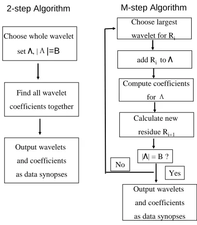
A. 2-step algorithm
The name of this algorithm comes from its 2-step mechanism adopted to derive the data synopsis (figure 4).
Choose whole wavelet
set , ||=B
Find all wavelet
coefficients together
Output wavelets
and coefficients
as data synopses
Choose largest
wavelet for Ri
Compute coefficients
for
Output wavelets
and coefficients
as data synopses add Rito
Calculate new
residue Ri+1
|| = B ?
Yes No
2-step Algorithm M-step Algorithm
Figure 4. Flow charts of2-stepandM-stepalgorithms
In Step A, we define the weighted dataAW to be a point-wise product of A and √Π , e.g. AW[i] = A[i]pΠ[i]. The algorithm selects a set of wavelets with the largest
B coefficients from the wavelet transform ofAW.
Step B computes the best coefficientsD[i]for the chosen
wavelets by solving the partial differential equation of the function described in Equation (1), e.g. ∂ǫ∂D(P[k)] = 0, ∀k∈[1, B].
The nice characteristics of the proposed algorithm is related to the fact that its approximation error is bounded by |Ab[i]−Ab∗[i]| = |AWb [i](1 − √1
Π[i])| after the first
iteration, and it will be reduced significantly at the second iteration.
The time and space complexity in Step A isO(n)for generatingAW fromAandW, as well as computing its wavelet transform, which is linear to the data size. Thus whether the Step B can be computed in linear time is critical to keep the overall cost low. The following lemma describes why Step B requires only linear time [9].
Lemma 1: For any given wavelet set with sizeB, the
best coefficient setD can be find in O(n+B3)time.
Proof Let the chosen wavelet set beΛ ={Ψ1, ...,ΨB}. The approximated dataR, defined as the product of the chosen wavelets and their coefficients, can be computed asR=Pi∈ΛD[i]Ψi.
As a consequence, the approximation errorǫ, defined as the L2 distance between original data and approximated data, can be written as:
ǫ = X
i
Π[i](A[i]−R[i])2
= Π⊗((D[1]Ψ1+...+D[B]ΨB−A)
while⊗is the inner product1 and⊙is the point-wise product of two vectors 2.
To find the bestD[i]that minimizes the error, we solve the following set of equations:
∂ǫ
∂D[1] = 0
... ∂ǫ
∂D[B] = 0
⇔P D=Q
in which,∂D∂ǫ[i] = 2Π⊗(Ψi⊙(D[1]Ψ1+...+D[B]ΨB−
A)) = 0. Notice that, the set of equations above can be written in matrix notation P D =Q whereP[i, j] =
Π⊗(Ψi⊙Ψj) andQ[i] = Π⊗(Ψi⊙A).
Since the time for solvingP D=Qis at mostO(B3), the dominate part of the time complexity ends to be the generation of the matricesP andQ. In the following, we propose an efficient approach to generate those matrices in O(n) based on the intuition that the computation of Ψi and Ψj collapses into three simple and standard cases, as shown in the following:
case 1: IfΨi andΨj do not overlap,
Ψi⊙Ψj= 0
case 2: IfΨi andΨj are the same, i.e.,i=j,
Ψi⊙Ψi = {1l, ...,1l}, where l is the length of Ψi’s
Support Interval, which is the non-zero parts ofΨi.
case 3: IfΨi coversΨj,
Ψi⊙Ψj=±ciΨj,ci is a constant that normalizeΨi,
named Normalization Factor, e.g., in figure 1,c7=√2. As a consequence, P[i, j] is either 0 (case 1), or the average value of ΠinΨi’s in the non-zero interval (case 2), or the wavelet transform coefficient ofΠscaled by+ci or−ci, where the sign depends on the relative position of
Ψj andΨi (case 3). For both case 2 and case 3, P[i, j]
can be computed directly from the wavelet transform of
Π. Since we can compute all values for P[i, j] directly from one wavelet transform of Π, we need only O(n) time to generate the entire matrix P.
Same observation hold true for the computation of the matrixQ. Indeed, allQ[i]values can be generated inO(n) as Q[i] = Π⊗(Ψi⊙A) = (Π⊙A)⊗Ψi, which is the coefficient of wavelet transform ofΠ⊙A.
In the following, we prove that the P D = Q is indeed solvable. First, let’s consider the case that not all coefficients ofΠare0in any of the chosen waveletΨi’s support interval, i= 1..B.
Then matrix P can be decomposed as the product of the matrixT and its transpose.
P =T T′
=
√
Π⊙Ψ1
...
√
Π⊙ΨB
√Π′⊙Ψ′
1, ...,
√
Π′⊙Ψ′
B
Since Ψ1, ...,ΨB are linear independent, and √Π⊙
1z=X
1×n⊗Y1×n⇔z=Pn
i=1X[i]Y[i] 2Z
1×n=X1×n⊙Y1×n⇔Z[i] =X[i]Y[i]
Ψi 6=~0,3 the rank(T) = rank(T′) = B. This means
thatrank(P) =Band thus theP matrix is non-singular. ThereforeP D=Qis solvable.
Second, let’s consider a more general case where allΠ are 0 for the entire Ψi’s support interval. To prove this case, we set all theD[i] = 0, and thus reduce the matrix
Pto be equal to(B−k)×(B−k), wherekis the number of suchΨis. Therefore, this equation is solvable.
Now let’s consider the computational time. In the worst case, we haveBequations withB variables, and thus we can solve all D[i] in O(B3) time. By adding the time required to generate the matricesP andQand solve the systemP D = Q, the total time complexity to compute the coefficients for a given wavelets is equal toO(n+B3).
In summary, the time complexity of the 2-step al-gorithm is O(n) for the computation of the wavelet transform andO(n+B3)for the computation of the best coefficients. The space complexity is O(n) for wavelet transform, andO(B2)for the coefficients selection. We want to remark to the reader that the O(n) space can be reused in the second step since the algorithm requires to keep the indexes of the B chosen wavelets only. As a consequence, the total time required for execution is expressed by O(n+ B3) while the space required is
O(max{n, B2}). Furthermore, its complexity becomes
linear to the data size n when B ≪ n, e.g. typical of standard database applications.
B. M-step Algorithm
The M-step algorithm represents an improvement of the 2-step algorithm based on the observation that the error obtained by the 2-step algorithm can be further reduced down by selecting new wavelets at each iterations (figure 4). The selection of the new wavelets is carried out in order to minimize the difference between the approximated data and the original data, termed residue and denoted asRiwhereirepresents the ith-iteration. The algorithm starts by setting the initial residueR0 =AW, and the chosen wavelet set to be the empty set. At each iterationi, the algorithm computes the wavelet transform for the current residueRi, chooses the wavelet Ψk with the largest coefficient and that does not belong to the chosen set. The new wavelet Ψk is added to the chosen set. The algorithm computes the new coefficient vector
D for all chosen wavelets by solving ∂D∂ǫ(P[k)] = 0. At this point, the new residueRi+1can be computed asRi+1 =
AW−Pik=1D[k]Ψk, and the algorithm is ready to enter into the next iteration i+ 1. The M −step algorithm continues until the cardinality of chosen wavelet set is equal toB.
At each step of this algorithm, every data point of the residue can change due to the new added wavelet. As a result, the algorithm needs to recompute the wavelet transform for everyRi. After B steps, the running time
adds up toO(nB+B4). The storage space isO(max{n+
B, B2}), because the algorithm needs to remember up to
B chosen coefficients.
A variation of the M-step algorithm is to choose I wavelets together at each step. This reduces the running time to O(nB/I+B4/I)at the cost of a degradation in accuracy. When I = B, this algorithm collapses to the
2-step algorithm.
A general comment about the two algorithms proposed in this section is related to their property of having the approximation error decreasing monotonously. If a “bad” wavelet is chosen at any iteration, the next step can always ignore its negative effects by setting its coefficient to 0. In Section VII we show how the two algorithms are able to efficiently reduce their estimation errors compared to
W-wav algorithm.
IV. NONUNIFORMRANGE-SUMS APPROXIMATION PROBLEM
The same idea presented in the previous section for the Point-wise approximation, can be easily generalized in the case of the Range-sum queries. For a data set
A with length n, there are n(n2+1) number of intervals and weights. A Naive method to solve the Range-sum approximation problem is to generate a new data set
A(new), in which every data pointA(i, j) represents an
interval extracted from the original dataAand computed as A(new)(i, j) = Pjk=iA[k]. As a consequence, it is straightforward to write the error function of the new data A(New) as ǫ(P)(A(New)) =Pi,jΠ[i, j](A(New)−
\
A(New))2, and thus find the wavelet synopsis using
meth-ods in point-wise approximation case.
Although the idea is simple, the complexity of this approach is high because the length ofA(New) isO(n2) and thus largely exceeds the synopses spaceB.
Because the complexity is determined by the number of intervals constituting the original dataA and the weights associated to each interval, in this Section we propose two new algorithms, named Data-mapping and
Weight-mapping, that generate new data vectors of sizen. To the
best of our knowledge, these algorithms are the first linear algorithms for arbitrary weights proposed in literature as now.
A. Data-mapping algorithm
The Data-mapping algorithm transforms the original Range-sum approximation problem into a simpler Point-wise approximation problem by introducing a simple data and weight transformation. Given the original dataA, we define a new data A(DM) obtained as the partial sum of
A, e.g.A(DM)[i] =Pik=1A[k]withA(DM)[0] = 0. By using the new dataA(DM), we can re-writeA(i, j) as the difference betweenA(DM)[j]andA(DM)[i−1], i.e.,
A(i, j) =A(DM)[j]−A(DM)[i−1]. As a consequence,
equation (2) can be looked as a function of new data
A(DM).
ǫR = X
i,j
Πi,j[(A(DM)[j]−A(DM)[i−1])
−(A(\DM)[j]−A(DM\)[i−1]]2
Thus we can obtain the expression of the new weights associated to the new data vectorA(DM) as follows:
Π(DM)[i] =Xi
k=1
p
Π[k, i] + Xn
k=i+1
p
Π[i+ 1, k] (4)
In order to minimize the error function and thus obtain the best wavelet coefficientsD, we calculate the derivative equation of the error function regard to D and set it to 0, e.g. ∂ǫ(R)(∂DA(DM)) = 0. As a consequence, the problem ends into solving a set ofB linear equations of the form for the general wavelet coefficient vectorD[k] (Equation 5).
If the B linear equations are solved one by one, the complexity of the procedure ends up to beO(n2B2+B3). In order to reduce the time complexity of this step, we propose to organize the Equations (5) in matrix notation of the formP D=Q, whereP[k, l] =Pi,jΠ[i, j](Ψk[j]−
Ψk[i])(Ψl[j]−Ψl[i])andQ[k] =Pi,jΠ[i, j](A(DM)[j]−
A(DM)[i−1])(Ψ
k[j]−Ψk[i−1]).
Then we construct a prefix sum table for Π[i, j] that helps to compute the weights for any interval (i, j) in constant time, so that the overall complexity can be reduced to O(n2 +B3). In the following paragraphs, we introduce the method that can reduce the cost from polynomial to linear.
We start with the evaluation of the cost to generate the matricesP andQ.
First, the matrixP can be computed inO(B2)due to two major observations:
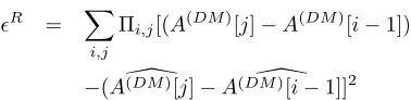
(i) There are only a constant number of intervals, i.e., less than 25 intervals, in which P[k, l]6= 0, since there are only5 non-zero intervals forΨk[j]−Ψk[i−1] and
Ψl[j]−Ψl[i−1](figure 5).
(ii) In these intervals,P[k, l]can be computed in constant time from Pi∈I,j∈JΠi,j, since normalization factor ck andcl are constants specified by onlyΨk andΨl. (iii) The computation of Pi∈I,j∈JΠi,j can be carried out in constant time with the help of a prefix sum table. The prefix sum table forΠi,j can be easily generated by adding every row of the tableΠi,j to its next to generate
P
i∈[1,k]Πi,j for each j, then adding every column to
its next right column to generatePi∈[1,k],j∈[1,l]Πi,j (see Figure 6 for more details). At the end of this process, the data is very well organized so that the computation of the Pi∈I,j∈JΠi,j for any interval I = [i1, i2] and
J= [j1, j2]needs only3operations:Π[[ij11,i,j2]2] = (Π[1[1,i,j2]2]−
Π[1[1,i,j2]1−1])−(Π[1[1,i,j12]−1]−Π[1[1,j,i11−−1]1]),where ΠIJ represent
P
i∈I,j∈JΠi,j.
Similarly, the matrixQcan be computed inO(B)time after constructing a prefix sum table of similar form for
D[1]X
i,j
Π[i, j](Ψ1[j]−Ψ1[i−1])(Ψk[j]−Ψk[i−1]) +...+
D[B]X
i,j
Π[i, j](ΨB[j]−ΨB[i−1])(Ψk[j]−Ψk[i−1])
= X
i,j
Π[i, j](A(DM)[j]−A(DM)[i−1])(Ψ
k[j]−Ψk[i−1]) (5)
1,1
1,2
2,2
1,n
2,n
n,n
…
…
…
… [1]
[1]
[1,2] [1,2] [1] [1,2]
[1,2] [1,n] [1] [1,n]
[1,n] [1,n] …
…
…
… [1]
[1]
[1,2] [2] [1] [2]
[1,2] [n] [1] [n]
[1,n] [n] …
(1) (2) (3)
Figure 6. Example of generation of a prefix sum table forP[k, l]
ak1 ak2
bk1 bk2
ak1 ak2bk1 bk2
al1 al2bl1 bl2 al1al2
bl1bl2
k
k
l
l
Ifi−1< ak1,
1:if i≤j≤ak2,Ψk[j]−Ψk[i−1] = c1
k
2:if bk1≤j≤bk2,Ψk[j]−Ψk[i−1] =−c1
k
else Ψk[j]−Ψk[i−1] = 0, sinceΨk[j] = Ψk[i−1] = 0. Ifak1≤i−1≤ak2,
3:if bk1≤j≤bk2,Ψk[j]−Ψk[i−1] =−c2
k
4:if bk2< j,Ψk[j]−Ψk[i−1] =−c1
k
else Ψk[j]−Ψk[i−1] = 0, sinceΨk[j] = Ψk[i−1] = c1
k.
Ifbk1≤i−1≤bk2,
5:if bk2< j,Ψk[j]−Ψk[i−1] = c1
k
else Ψk[j]−Ψk[i−1] = 0, sinceΨk[j] = Ψk[i] =−c1
k.
Figure 5. 5intervals in whichΨk[j]−Ψk[i−1]6= 0(ck is the normalization factor forΨk)
l
As a result, the time required to generate the matrix P and Q is only O(B2) with the help of their prefix sum tables, which needO(n(n2+1))to construct. Therefore the total cost is successfully reduced from O(n2B2+B3) to O(n2+B3), including the O(B3) time for solving equationP D=Q.
B. Weight-mapping algorithm
In some scenario, for example, when monitoring the trends of data changes through its approximation, one may prefer to approximate the original data A instead of its
prefix sum dataA\(DM). In this case, we need to find the new weights that are associated withA, since the original weightsΠ[i, j]are given for interval[i, j].
Similar to the data-mapping scenario, the new weights can be derived from the error function (Equation 2) by substitutingA(i, j)withPi≤k≤jA[k], i.e.,Π(W M)[k] =
P
i∈[1,k],j∈[k,n]
p Π[i, j]
Now the new error functionP D = Q, composed by equations of the type ∂D∂ǫ(R[k)] = 0, can be expanded as the following (Equation 6):
D[1]X
i,j
Π[i, j]Ψk(i, j)Ψ1(i, j) +
D[2]X
i,j
Π[i, j]Ψk(i, j)Ψ2(i, j)
+...+
D[B]X
i,j
Π[i, j]Ψk(i, j)ΨB(i, j)
= X
i,j
Π[i, j]Ψk(i, j)A(i, j) (6) As for the weight mapping algorithm, there is a constant number of intervals, e.g. in this case 13 intervals, in which Ψk(i, j)Ψl(i, j) 6= 0. In these intervals, if we compute the prefix table for each of the iΠ[i, j], jΠ[i, j], i2Π[i, j], j2Π[i, j], ijΠ[i, j], and
Π[i, j]A(i, j), then the matricesP andQcan be generated inO(B3)time. As a result, the total cost for the Weight-mapping algorithm is stillO(n2+B3), due to the prefix table construction timeO(n2)and equation solving time
O(B3).
Data-Mapping Algorithm
Compute prefix sum data A(DM)from A
Compute new weight
(DM) for A(DM)from
Choose wavelets from wavelet transform of
new weighted data
(DM) A(DM)
Optimize the coefficients for chosen wavelets on original error function,
and return them as data synopses
Compute new weight
(WM) for A from
Choose wavelets from wavelet transform of
new weighted data
(WM) A
Optimize the coefficients for chosen wavelets on original error function,
and return them as data synopses Weight-Mapping Algorithm
Figure 7. Data-mapping and Weight-mapping algorithm
total space is bounded by O(n2+B2).
V. TRACKING DYNAMIC CHANGES OF WEIGHTS AND DATA
In the previous sections III and IV we introduced the algorithms to generate the data synopses. As we discussed in the introduction, in databases, data and weights might change over time. In this section we discuss how to keep the data synopses accurate over time when dealing with dynamic data and weights.
For Point-wise approximation, when a data point or a weight value changes, only up tolog(n)wavelets need to change. By comparing them with the chosenB wavelets, the new wavelets can be found inmax(log(n), B)time. Thus, the updating time is bounded by O(log(n) +B3) withO(B3)time required to find the new coefficients.
For Range-sum queries, the dominant part of the cost is associated to the prefix sum table construction time, that requires O(n2). In the following we propose an incremental multi-step method to keep the overall cost below O(n+B3) while requiring an extra O(n) space to store updates. We describe the new method in the following sections for the data-mapping and the weight-mapping algorithms for both the cases of dynamic data and weights.
A. Data change in data-mapping algorithm
For the data mapping algorithm, a change of a single data point may cause the change of up tonvalues in the prefix sum dataA(DM), depending on the location of the data point.
First, the method needs to recompute the wavelet trans-form of A(DM), which requires O(n) time. Now, since
A(DM)is not involved in the generation of the matrixP,
the data change does not require any re-computation of the matrix P (see Equation (5)). However this is not the case for the vector Q.
As a second step, we need to re-compute the vectorQ. It is straightforward to notice that if we update the prefix
sum table for Q, i.e. prefix sum table of Π[i, j]A(i, j), and compute Qdirectly from the new table, the cost of its re-computation will beO(n2), due to the fact that all
O(n2) entries [1,j]
[1,i] with i ≥t or j ≥t will be affected
by such update.
Next, we show that by considering some inner prop-erties of the vectorQ, the method can further reduce its re-computation time toO(B)in case of a single data point change, or more generally, to O(B +x)for x changes. Recall that there is only a constant number of intervals in whichQ[k]6= 0. Let {I, J} be these non-zero intervals, andvI,J be one of theQ[k]values specific for the interval
I, J, i.e. Q[k] can be seen as the sum of vI,Js over all intervals{I, J}s, i.e.,Q[k] =PI,JvI,J.
Now, the new Q′[k] can be computed from the old vectorQ[k] in constant time. To prove that, let’s assume that the difference between the new data valueA′[t] and the old data valueA[t]isδAt =A′[t]−A[t].
We start from the update in one of its non-zero interval
I = [i1, i2], J = [j1, j2]. Because only when t ∈ I, J, the new update will be reflected in the partial sum data, that is wheni ≤j < t ort < i≤j, A′(i, j) =A(i, j), and wheni≤t≤j,A′(i, j) =A(i, j) +δAt.
Therefore we can separate the new valuev′I,J into two parts: one includesA′[t], i.e.,i∈I∩[1, t], j∈J∩[t, n], and the other does not, i.e.,i ∈I∩[1, t), j ∈J∩[1, t) andi∈I∩(t, n], j∈J∩(t, n].
Thus, v′I,J can be computed from vI,J in O(1) time (Equation (7)) with the help of the prefix sum table of
Π[i, j]. As a consequence Q′[k] can be computed from
Q[k] in constant time, since the number ofI, Js is only a small constant. Therefore the total update time forQis
O(B).
More generally, when there are xnumber of changes in the data, the total updating time of Q is O(B +x) obtained by adding the changes toQone by one.
When x < n, we compute Q[k] using the original
table, then update it to Q′[k]: The update time contains the following.
(1) Recompute wavelet coefficients:O(n).
(2) ChooseB wavelets and computeP andQ:O(B2). (3) UpdateQtoQ′ for allδtA:O(B+x).
(4) Solve new equationP D=Q′: O(B3).
When the changes reach n, we recompute the prefix sum tables, and run the algorithm on the new tables, which takesO(n2+B3).
So the amortized cost is O(n + B3), because
O(1
n[
Pn−1
x=1(n+B3+x) + (n2+B3)]) =O(n+B3)
B. Data change in weight mapping algorithm
The only difference between the weight mapping and the data mapping resides in the first step of the method. When A[t] changes, the time involved in finding new wavelets is O(log(n)), instead of O(n). In the second step, only the vector Q’s prefix table changes with
v′
I,J =
X
i∈I∩[1,t)
j∈J∩[1,t)
Π[i, j]A(i, j) + X
i∈I∩(t,n]
j∈J∩(t,n]
Π[i, j]A(i, j) + X
i∈I∩[1,t]
j∈J∩[t,n]
Π[i, j]A′(i, j)
= X
i∈I∩[1,t)
j∈J∩[1,t)
Π[i, j]A(i, j) + X
i∈I∩(t,n]
j∈J∩(t,n]
Π[i, j]A(i, j) + X
i∈I∩[1,t]
j∈J∩[t,n]
Π[i, j]A(i, j) + X
i∈I∩[1,t]
j∈J∩[t,n]
Π[i, j]δA t
= X
i∈I
j∈J
Π[i, j]A(i, j) + (min(i2, t)−i1)∗(j2−max(j1, t))δA t
X
i,j
Π[i, j]
= vI,J+ (min(i2, t)−i1)∗(j2−max(j1, t))δA t
X
i,j
Π[i, j] (7)
O(1
n[
Pn−1
x=1(log(n)+B3+x)+(n2+B3)]) =O(n+B3).
If a weight value Π[i, j] changes to Π′[i, j], where
P
i,jΠ′[i, j] =
P
i,jΠ[i, j] +δΠi,j, bothP[k, l]and Q[k]
need to be updated.
By applying the same method in data updates, we can compute P[k, l] and Q[k] from the original prefix sum tables, and addδi,jΠ orδΠi,jA(i, j)to computeP′[k, l]and
Q′[k].
C. Weight change in data mapping algorithm
In the data mapping algorithm, a single update in the original weights Π leads to at most two changes in Π(DM) (Equation (4)). Thus only O(log(n)) wavelet coefficients need to be re-calculated. Because of these new coefficients, the Equation P D = Q has to be re-generated, which requiresO(B2)time. Similar to the case of the data changes, forxchanges in weights, the update time from P D = Q to P′D = Q′ is O(B2+x) for
P[k, l] and O(B +x) for Q[k]. The time required to solve the equation P D = Q is then O(B3). Therefore, the amortized time forxupdates is O(n1[Pnx−=11(log(n) +
B3+x) + (n2+B3)]) =O(n+B3).
D. Weight change in weight mapping algorithm
The only difference between the data-mapping and the weight mapping regards the fact that a single update in weights may cause up to n changes in weighted data
Π(W M) ⊙A. Thus, we need O(n) wavelet transform
time, and the amortized cost is stillO(n+B3), because
O(1
n[
Pn−1
x=1(n+B3+x) + (n2+B3)]) =O(n+B3)
In summary, our incremental method exploits the previ-ous computed values residing in the database to compute the new values, avoiding the new values to be calculated from scratch. Therefore, this method can successfully reduce the update cost for both data-mapping and weight-mapping from linear to sub-linear in time.
VI. SPECIALCASES FORRANGE-SUMWEIGHTS In the previous sections, we discussed the most general cases of weights, in which each point of the weight may differ from the other ones. However, there are some special scenarios in which weights may have some nice
structures that, if fully exploited, might help to further reduce the running time. In this section we discuss three of them:Uniform Weights, Uniform Length Weightsand
Hierarchical Sum Weights.
Uniform weights This case, also known as “unweighted
range-sum problem”, assume that there is only one unique weight for all intervals, i.e.∀i, j, k, l,Π[i, j] = Π[k, l].
Uniform length weights This case assume that the
weights are same if their interval lengths are the same, i.e.
Π[i, j] = Π[k, l], ifj−i=l−k, andΠ[i, j] = Π[k, l]+h, ifj−i=l−k+ 1, wherehis the unit weight difference. In this context, we useΠ|l|to represent the weight for an interval with lengthl, such thatΠl= Π1+ (l−1)∗h.
Hierarchical sum weights This case assume the
exis-tence of a unique weightΠi,ifor eachi. All other weights can be derived from them, i.e.Πi,j=Pjk=iΠk,k.
Recall that in section IV, after we constructed the prefix tables, the computational costs for generating P, Q and solvingP D =Q were completely independent fromn. The dominant part of the overall costO(n2+B3)turned out to be the table construction timeO(n2).
For these special cases, where weights for different points and intervals are not totally independent, we will show that we can further reduce down the table size from
O(n2) to O(n) by exploiting the existence of an inner
dependency between weights and intervals.
Before starting, we introduce a simple but important lemma that we will use later to analyze the cost reduction.
Lemma 2: Given a generic vector V =
{V[1], V[2], ..., V[n]}, the sum of any arithmetic
series of its entries, i.e. f(k, d, i, j) = kV[i] + (k +
d)V[i+ 1] +...+ (k+ (j−i)d)V[j], can be computed inO(1)time after O(n) preprocessing time.
Proof We generate the following two prefix sum tables
from vectorV inO(n)time.
SV
1 ={V[1], V[1] +V[2], ..., V[1] +...+V[n]}
SV
2 ={V[1], V[1] + 2V[2], ..., V[1] +...+nV[n]}
f(k, d, i, j)
= kV[i] +...+ (k+ (j−i)d)V[j]
= kV(i, j) +d(V[i+ 1] +...+ (j−i)V[j]) = k(SV
1[j]−S1V[i−1]) +d(S2V[j]−S2V[i])
−id(SV
1[j]−S1V[i]) (8)
For all these special cases, the prefix sum tables of size
O(n2) can be reduced to a vector of size O(n), which
is similar to S1V, S2V. Furthermore, with the help of these new prefix vectors the entries of both matrixPand vector
Qcan still be computed inO(1) time. Running time for all other parts of the algorithm remains same, except the table construction time is reduced from O(n2) toO(n). So the total running time is reduced to O(n+B3).
In this section, we discuss only the prefix vector for
Q, i.e., the prefix vector ofPi∈I,j∈JΠ[i, j]A(i, j). The prefix vector for P (prefix vector ofPi∈I,j∈JΠi,j) can be considered as a special case of the previous one when
A(i, j) = 1. In the following we use the uniform weight case as an example to show how to reduce the prefix table size, and summarize the results for all three cases in table II.
We also want to remark to the reader that we need to consider only two cases of overlapping intervals, e.g.,
I∩J =φandI=J, to further simplify our computation, because if I∩J 6= φ, and I 6= J, then j1 ≤ i2. This interval can be divided into 3 parts: I1 = [i1, j1−
1], J1 = [j1, j2], I2 = [j1, i2], J2 = [j1, i2] and
I3 = [j1, i2], J3 = [i2 + 1, j2]. In these new intervals
I1∩J1 =φ, I2 = J2 andI3∩J3 =φ. This division creates 3 subintervals, each of them can be solved by using the prefix vectors defined in the table I.
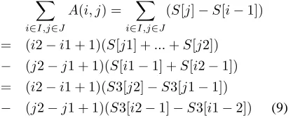
Example: prefix table reduction for uniform weights
In the uniform weight case, Πi,j is a constant for all intervals. We define S[i] =Pik=1A[k].
X
i∈I,j∈J
A(i, j) = X
i∈I,j∈J
(S[j]−S[i−1])
= (i2−i1 + 1)(S[j1] +...+S[j2])
− (j2−j1 + 1)(S[i1−1] +S[i2−1]) = (i2−i1 + 1)(S3[j2]−S3[j1−1])
− (j2−j1 + 1)(S3[i2−1]−S3[i1−2]) (9) where interval I = [i1, i2], J = [j1, j2], and S3 is defined in table I.
As a result, if we pre-compute a prefix sum vectorS3, the prefix sumPi∈I,j∈JA(i, j)for any intervalI, J can be computed in constant time as in equation (9). Therefore
P
i∈I,j∈JΠ[i, j]A(i, j) = Π[i, j] P
i∈I,j∈JA(i, j) can
be computed in O(1) time fromPi∈I,j∈JA(i, j) since
Π[i, j]is a constant.
In this section, we have shown that our algorithm can be easily applied to different special weights, with a dramatic complexity reduction. This is because our algorithms
TABLE I. PREFIX SUM TABLES
S1={Π[1,1],Π[1,1] + Π[2,2], ...,Π[1,1] +...+ Π[n, n]} S2={Π[1,1],Π[1,1] + 2Π[2,2], ...,Π[1,1] +...+nΠ[n, n]} S3={S[1], S[1] +S[2], ..., S[1] +...+S[n]}
S4={S1[1]S[1], S1[2]S[2], ..., S1[n]S[n]} S5={S1[0]S[1], S1[1]S[2], ..., S1[n−1]S[n]} S6={S2[1]S[1], S2[2]S[2], ..., S2[n]S[n]} S7={Π1,1S3[1],2Π2,2S3[2], ...., nΠn,nS3[n]} S8={Π1,1S3[1],Π2,2S3[2], ....,Πn,nS3[n]} S9={S3[1], S3[1] +S3[2], ..., S3[1] +...+S3[n]} S10={S3[1], S3[1] + 2S3[2], ..., S3[1] +...+nS3[n]}
capture the properties of the real complex component, i.e., theO(n2)weights, through its prefix sum table. When the weights can be simplified, the cost of our algorithm can be simplified accordingly.
VII. EXPERIMENTS
In this section, we show the accuracy and efficiency of our method on different data sets. We use the relative error defined asRE= ǫB
ǫ0 =
P
iPΠ[i](A[i]−Ab[i])2 iΠ[i](A[i])2
for point-wise approximation, and RE = ǫB
ǫ0 =
P
i,jΠi,j(A[i,j]−Ab[i,j])2 P
i,jΠi,j(A[i,j])2
for range-sum approximation, where ǫB is the absolute approximation error withBbuckets. The experiment was done by using a Linux machine with 2.80GHz processor and 2047 MB memory.
A. Point-wise queries
In this section, we compare the 2-step, M-step and W-wav algorithms using both synthetic and real data sets. In these experiments, we setI = 1for the M-step method. For other I values, the approximation error is between error of 2-step, and error of M-step withI= 1.
a) Synthetic Data: The synthetic data set contains
4096data points, and they are extracted from a normal, an exponential and a uniform distribution. The weights are extracted from a zipf distribution withα= 0.2,0.5 and0.8. In the following we compare the 2-step and M-step algorithms for Point-wise approximation against the W-Way algorithm in terms of accuracy,efficiency, time
andskewness.
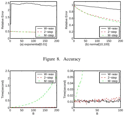
Accuracy Accuracy results are shown in Figure 8(a)
when the data set is extracted from an exponential dis-tribution with parameter λ = 0.01. Major consideration to make is related to the shape of these curves: the error for W-wav jumps to 2.5ǫ0 and remains there even after
B= 200 while both the 2-step and M-step always keep the error under 0.5ǫ0. The reason of such behavior is related to the fact that when a data set contains very large values, W-wav takes more wavelets from this region than necessary, while the 2-step and M-step algorithms can set
0as coefficients for the “unwanted” wavelets.
Efficiency Efficiency results are shown in Figure 8(b)
when the data set is extracted from a normal distribution with mean=10and variance=100. Notice here the 2-step and M-step algorithms are capable to reduce the error to
TABLE II.
WEIGHT REDUCTION TABLE
I∩J LSj= ((L2+ 1)Π|L1|+L2(L22+1)hS3[j1 +L2]−[(Π|1|+h(L1−1))(S9[j1 +L2]
=φ −S9[j1−2]) +h[(1−j1)(S9[j1 +L2]−S9[j1−1]) + (S10[j1 +L2]−S10[j1−1]) I∩J LSi= Π|L1|(S9[i1 +L2]−S9[i1−1]) +h(1−i1)(S9[i1 +L2−1]−S9[i1−1])
=φ +(S10[i1 +L2−1]−S10[i1−1]) + Π|L1|L2(L22+1)hS3[i1−1] I=J LSj= ((L2+ 1)Π|1|+L2(L22+1)hS3[i2]−[Π|1|(S9[i2]−S9[i1−2])
+h[(1−i1)(S9[i2]−S9[i1−1]) + (S10[i2]−S10[i1−1])
I=J LSi= Π|1|(S9[i2]−S9[i1−1]) +h(1−i1)(S9[i2−1]−S9[i1−1])
+(S10[i2−1]−S10[i1−1]) + Π|L1|L2(T22+1)hS3[i1−1]
I∩J HSj= [(1−i1)(S1[i2]−S1[i1−1]) + (S2[i2]−S2[i1−1])](S3[j2]−S3[j1−1])
=φ +(i2−i1 + 1)[S4[j2]−S4[j1−1] + (2S1[j1−1]−S1[i2])(S3[j2]−S3[j1−1])] I∩J HSi= (j2−j1 + 1)[S1[j1−1](S3[i2]−S3[i1−1])−(S5[i2]−S5[i1−1])]
=φ +[(j2 + 1)(S1[j2]−S1[j1−1])−(S2[j2]−S2[j1−1])]S[i1,i2] I=J HSj= (S6[i2]−S6[i1−1])−S2[i1−1](S3[i2]−S3[i1−1])
I=J HSi= (i2 + 1)(S8[i2]−S8[i1−1])−(S7[i2]−S7[i1−1]) + (i2−i1 + 1) ∗(S1[i2]−S1[i1−1]) +i1(S1[i2]−S1[i1−1])−(S2[i2]−S2[i1−1])
LSjandHSjstands forP
i∈I,j∈JΠi,jPjk=1A[k], in uniform length weights case and hierarchical sum weights case;
LSiandHSistands forP
i∈I,j∈JΠi,jPi
k=1A[k]in those cases.L1is start interval length,L1=j1−i1 + 1.L2is max shift length,L2=min{i2−i1, j2−j1}.
0 50 100 150 200
0 0.5 1 1.5 2 2.5
Relative Error
(a) exponential[0.01] W−wav 2−step M−step
0 50 100 150 200
0 0.2 0.4 0.6 0.8 1
Relative Error
(b) normal[10,100] W−wav 2−step M−step
Figure 8. Accuracy
0 50 100 150 200
0 0.5 1 1.5 2 2.5
B
Time(second)
W−wav 2−step M−step
0 50 100
0 0.01 0.02 0.03 0.04 0.05 0.06
B
Time(second)
W−wav 2−step M−step
Figure 9. Efficiency
as high as 0.85ǫ0. This is caused by cancellation among overlapped wavelets using the original coefficients. The 2-step and M-step algorithms can lower this side-effect by finding the best coefficient for each wavelet.
Time In Figures 9 we show the running time of the
three algorithms M-step method requires a very large running time. It reaches 2 second when B = 200 (figure 8(a)). With the figure at a smaller scale (fig-ure 8(b)),the running time for W-wav is O(n), and is constant for allB. Running time for the 2-step is bounded by O(n+B3). For B3< n, that isB <16, there is no difference of running time between the 2-step and W-wav algorithms. Even whenB reaches200,2003≫4096, the extra time for the 2-step is only 0.05second.
Skewness Last, in Figures 10(a) and 10(b) we compare
the three algorithms while changing the weight distribu-tions (zipf 0.2, 0.5 and 0.8). The data set is extracted
0 100 200
0.4 0.6 0.8 1
zipf 0.2
B
Relative Error
0 100 200
0.4 0.6 0.8 1
zipf 0.5
B
Relative Error
0 100 200
0.4 0.6 0.8 1
zipf 0.8
B
Relative Error
W−wav 2−step M−step
W−wav 2−step M−step
W−wav 2−step M−step
(a)Normal[10,100]data
0 100 200
0 0.05 0.1 0.15 0.2
zipf 0.2
B
Relative Error
0 100 200
0 0.05 0.1 0.15 0.2
zipf 0.5
B
Relative Error
0 100 200
0 0.05 0.1 0.15 0.2
zipf 0.8
B
Relative Error
W−wav 2−step M−step
W−wav 2−step M−step
W−wav 2−step M−step
(b)Uniform[1,10]data Figure 10. Skewness
from normal and uniform distributions. Important to no-tice here how the performance of the W-wav method decreases as weights become more skewed, e.g. from to zipf 0.8. This characteristic can be explained because W-wav method combines weights with wavelets. The more skewed the weights are, the higher will be the probability that wavelets with heavy weights will be used. On the other hands, both the 2-step and M-step algorithms can ignore those exaggerated wavelets by setting their coefficients to0.
b) Real Data: In order to validate the above
0 2 4 6 8 x 10⁴ 0 0.5 1 1.5 2 2.5
3x 10
6 Data Value
object ID
0 2 4 6 8
x 104 0 0.01 0.02 0.03 0.04 0.05 Query Weights object ID
0 500 1000
0 0.5 1 1.5 2 2.5 B Relative Error W−wav 2−step M−step
0 50 100
0 2 4 6 8 10 B Time(second) W−wav 2−step M−step
Figure 11. Relative error compare for world cup data
response size of the subject. Weights correspond to the number of queries for each data point after normalization. In this case as well, we observe the same dynamics as before for the relative error; the W-wav method provides a relative error above2ǫ0at first, then it is slowly reduced to
0.35ǫ0 atB= 600 and remains there throughB= 1000
(Figure 11). The 2-step algorithm reduces its error to
0.35ǫ0 with B = 13while the M-step reduces its error
to0.35ǫ0 with onlyB = 9. The running time difference between the 2-step method and the W-wav method is very small when B <100.
B. Range-Sum Approximation
In this section we compare our proposed algorithm, the data mapping method, the weight mapping method with the following method, including the Naive method described in Section IV.
. Data Our data-mapping method, whereP Π(DM)[i] =
i
k=1
p
Π[k, i] +Pnk=i+1pΠ[i+ 1, k]
. Data2 A simple straight forward data-mapping method,Π(DM)[k] =P1≤i≤j≤kpΠ[i, j]
. Weight Our weight-mapping method,P Π(W M)[k] =
i∈[1,k],j∈[k,n]Π[i, j]
. Weight2 A simple subtractive weight-mapping method,Π(W M) = Π(DM)[i]−Π(DM)[i−1], we useΠ(DM) in Data
. Naive Naive method with new signal X = {A(0,0), A(0,1), ..., A(n−1, n−1)}.
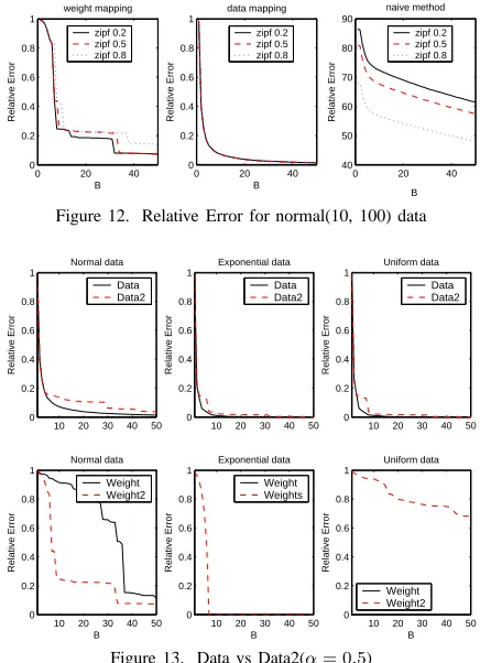
TheNaivemethod produces relative errors in the range
40−90while Datapushes it down below1(Figure 12). The reason of this dynamic is due to the fact that B is too small for data set with O(n2) length. In Figure 13 we compare the Data and Data2 methods in terms of their accuracy. We highlight how Data performs better than Data2over different data sets, because the weights computed by Data2 are not as accurate as the weights computed byDatathat are derived directly from the error functions.
0 20 40
0 0.2 0.4 0.6 0.8 1 weight mapping B Relative Error
0 20 40
0 0.2 0.4 0.6 0.8 1 data mapping B Relative Error
0 20 40
40 50 60 70 80 90 naive method B Relative Error zipf 0.2 zipf 0.5 zipf 0.8 zipf 0.2 zipf 0.5 zipf 0.8 zipf 0.2 zipf 0.5 zipf 0.8
Figure 12. Relative Error for normal(10, 100) data
10 20 30 40 50 0 0.2 0.4 0.6 0.8 1 Normal data Relative Error
10 20 30 40 50 0 0.2 0.4 0.6 0.8 1 Exponential data Relative Error
10 20 30 40 50 0 0.2 0.4 0.6 0.8 1 Uniform data Relative Error
10 20 30 40 50 0 0.2 0.4 0.6 0.8 1 Relative Error B Normal data
10 20 30 40 50 0 0.2 0.4 0.6 0.8 1 B Relative Error Exponential data
10 20 30 40 50 0 0.2 0.4 0.6 0.8 1 B Relative Error Uniform data Weight Weight2 Weight Weights Data Data2 Data Data2 Data Data2 Weight Weight2
Figure 13. Data vs Data2(α= 0.5)
For exponential and uniform data, Weight is much better thanWeight2. The error is almost0. But in normal data, it is worse (Figure 13). The reason is thatWeight2
focuses only on intervals start withi,i+ 1,i−1 or ends withi,i−1,i+1, but ignores all other intervals[i, j]that cover it. For the exponential and uniform data set, some intervals may contain very different values from others. Ignoring those intervals will incur large errors. Weight
considers all intervals that cover the data point, but it exaggerates the middle part of the signal. For normal data, all intervals are similar, exaggeration of certain intervals will make them unfairly important than others. This causes error.
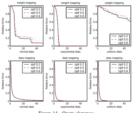
In Figure 14 we show relative error ofDataandWeight
method as a function of skewness of weights (zipf 0.2, 0.5 and 0.8). As a consequence, the skewness of the queries does not affect the algorithm accuracy because bothData
and Weight method sums certain Π[i, j]s together to compute a new weight. This summation cancels out the skewness effect.
VIII. CONCLUSION
0 20 40 0
0.2 0.4 0.6 0.8 1
weight mapping
Relative Error
normal data
0 20 40
0 0.2 0.4 0.6 0.8 1
weight mapping
exponential data
Relative Error
0 20 40
0 0.2 0.4 0.6 0.8 1
weight mapping
uniform data
Relative Error
0 20 40
0 0.2 0.4 0.6 0.8 1
normal data
Relative Error
data mapping
0 20 40
0 0.2 0.4 0.6 0.8 1
Relative Error
data mapping
exponential data
0 20 40
0 0.2 0.4 0.6 0.8 1
uniform data
Relative Error
data mapping
zipf 0.2 zipf 0.5 zipf 0.8
zipf 0.2 zipf 0.5 zipf 0.8
zipf 0.2 zipf 0.5 zipf 0.8 zipf 0.2
zipf 0.5 zipf 0.8 zipf 0.2
zipf 0.5 zipf 0.8
zipf 0.2 zipf 0.5 zipf 0.8
Figure 14. Query skewness
original data. This takes extraO(B3)time, but improves accuracy significantly. How to find the optimal wavelets for original data is still an open problem.
ACKNOWLEDGMENT
We thank Muthu Muthukrishnan for numerous inspir-ing discussions concerninspir-ing this work, and reviewers for their detailed comments.
REFERENCES
[1] Y. Matias and D. Urieli, “Optimal workload-based weighted wavelet synopses,” in ICDT, 2005.
[2] A. Aboulnaga and S. Chaudhuri, “Self-tuning Histograms: Building Histograms Without Looking at Data,” SIGMOD, 1999.
[3] N. Bruno, S. Chaudhuri, and L. Gravano, “STHoles: A Multidimensional Workload-Aware Histogram,” Tech. Rep., 2001.
[4] C. M. Chen and N. Roussopoulos, “Adaptive Selectivity Estimation Using Query Feedback,” 1994, pp. 161–172. [5] V. Ganti, M.-L. Lee, and R. Ramakrishnan, “ICICLES:
Self-Tuning Samples for Approximate Query Answering,” 2000, pp. 176–187.
[6] A. C. Konig and G. Weikum, “Combining histograms and parametric curve fitting for feedback-driven query result-size estimation,” in VLDB, 1999.
[7] V. Markl, G. M. Lohman, and V. Raman, “Leo: An auto-nomic query optimizer for db2,” in IBM Systems Journal, vol. 42, 2003.
[8] S. Muthukrishnan, M. Strauss, and X. Zheng, “Workload-optimal histograms on streams,” in ESA, 2005.
[9] S. Muthukrishnan, “Subquadratic algorithms for workload-aware haar wavelet synopses,” in FSTTCS, 2005. [10] N. Koudas, S. Muthukrishnan, and D. Srivastava, “Optimal
histograms for hierarchical range queries,” in PODS, 2000. [11] S. Muthukrishnan and M. Strauss, “Rangesum histograms,”
in SODA, 2003.
[12] N. Thaper, S. Guha, P. Indyk, and N. Koudas, “Dynamic multidimensional histograms,” in SIGMOD, 2002. [13] K. Chakrabarti, M. Garofalakis, R. Rastogi, and K. Shim,
“Approximate query processing using wavelets,” vol. 10, no. 2-3.
[14] M. Garofalakis and A. Kumar, “Deterministic wavelet thresholding for maximum-error metrics,” in PODS, 2004, pp. 166–176.
[15] Y. Matias and D. Urieli, “Optimal wavelet synopses for Range-Sum Queries,” in Proceedings of the 1st ACM
Conference on Computer and Communications Security,
Nov. 1993.
[16] Y. Matias, J. S. Vitter, , and M. Wang, “Wavelet-Based Histograms for Selectivity Estimation,” in SIGMOD, 1998. [17] Y. Matias, J. S. Vitter, and M. Wang, “Dynamic
Mainte-nance of Wavelet-Based Histograms,” in VLDB, 2000. [18] S. Guha and B. Harb, “Wavelet Synopsis for Data Streams:
Minimizing Non-Euclidean Error,” KDD, 2005.
[19] S. Guha, N. Koudas, and D. Srivastava, “Fast Algorithms for Hierarchical Range Histogram Construction,” 2002. [20] Http://ita.ee.lbl.gov/html/contrib/WorldCup.html.
[21] S. Chen and A. Nucci, “Nonuniform Compression in Databases with Haar Wavelet,” 2007, pp. 223–232. [22] M. Garofalakis and P. B. Gibbons, “Wavelet Synopses with
Error Guarantees,” 2002, pp. 476–487.
[23] S. Guha and B. Harb, “Approximation Algorithm for Wavelet Transform Coding of Data Stream,” in SODA, 2006.
[24] A. C. Gilbert, Y. Kotidis, S. Muthukrishnan, and M. J. Strauss, “Surfing Wavelets on Streams: One-Pass Sum-maries for Approximate Aggregate Queries,” 2001. [25] L. Lim, M. Wang, and J. S. Vitter, “SASH: A
Self-Adaptive Histogram Set for Dynamically Changing Work-loads,” 2003.
Su Chen is currently a Ph.D. candidate at Rutgers, The State University of New Jersey, USA. She received her MS degree in computer science from Fudan University, Shanghai, China, in 2001. Her research interests are massive data analysis, with applications in both network and database area, including mod-eling, approximation, mining and compression for both online and offline data processing.
![Figure 5. 5 intervals in which Ψk[j] − Ψk[i − 1] ̸= 0 (ck isthe normalization factor for Ψk)](https://thumb-us.123doks.com/thumbv2/123dok_us/8356383.1669071/7.595.66.284.315.582/figure-intervals-psk-psk-isthe-normalization-factor-psk.webp)