Abstract—This paper presents methods that utilize multi-core PC to perform large-scale MOSFET circuit and transient sensitivity simulations in parallel. A very coarse-grained parallel computing scheme, called Combining Simulation Method (CSM), is proposed for both circuit and transient sensitivity simulations. Relaxation-based algorithms have been utilized as simulation algorithms in CSM, in which only minor modifications for algorithm codes are needed. All proposed methods have been implemented and tested in multi-core PCs. Experimental results justify good speedups and accurate results can be obtained.
Index Terms—circuit simulation, parallel computing, relaxation-based, sensitivity computation
I. INTRODUCTION
Undertaking circuit simulation is very important in IC design community. Accurate approaches to solve circuit simulation problem include the “standard” simulators (such as SPICE) and relaxation-based simulators (such as RELAX [1], and SPLICE [2]). There exist faster simulation approaches using simpler simulation models (such as piecewise-linear model and switch-level model). But they only provide related coarse waveforms. The trade-off between the solution accuracy and simulation speed firmly exists.
In this paper, we propose PC-based parallel-computing strategies to raise the calculation efficiency directly and then break the trade-off mentioned above. Since multi-core PCs are very popular today, the success of this paper has practical values. We propose parallel-computing strategies for MOSFET circuit simulation as well as for sensitivity simulation. Our basic idea is to ask various processors to simulate different portions of the simulated circuit and then combine “sub-waveforms”. We call this strategy the Combining Simulation Method (CSM). Partitioning the simulated circuit into portions is important in CSM. We find that simulation-on-demand (SOD, i.e. only simulate subcircuits contributing to wanted outputs) can be used to partition for CSM in circuit simulation case, and direct dividing design parameters can be used to partition for CSM in sensitivity simulation case.
Backward-traversing Waveform Relaxation (BTWR) [3] is a specialized relaxation-based algorithm that simulates subcircuits by traversing subcircuits from the rear end to front end backwardly. So, it has the function of SOD. We will
Manuscript received July 30, 2012; revised September 3, 2012. This work was supported by the National Science Council of Taiwan under Grant NSC 101-2221-E-034-010
Chun-Jung Chen is with the Dept. of Computer Science, Chinese Culture University, Taipei, Taiwan (e-mail: [email protected]).
use SOD of BTWR to divide. Iterated Timing Analysis (ITA) [2] is another relaxation-based algorithm, and it has been used in commercial FAST SPICE programs. The SOD function can be added to it in order to use CSM. However, the SOD in ITA can be dependent on static signal flows. We also find that the Direct Approach for solving transient sensitivities can be used in CSM, too. The sensitivity circuit with respect to a design parameter is independent to those with respect to other design parameters. So, each sensitivity circuit is an independent portion in using CSM. Sensitivity computations can be naturally implemented in CSM.
The proposed methods all have been implemented. Experiments are made to justify their effects. The outline of this paper is as follows. In Section 2, the methods for solving circuit/sensitivity simulations are described, including BTWR, ITA, and Direct Approach sensitivity simulation. In Section 3, CSM is illustrated. Section 4 shows experimental results to demonstrate effects of proposed methods. Finally, conclusions are made in Section 5.
II. BTWR,ITA AND SENSITIVITY COMPUTATIONS
A. BTWR Algorithm
One of the fundamental circuit simulation algorithms of this work is BTWR, which is relaxation-based [1, 2]. The two famous algorithms of this class of algorithms are WR (Waveform Relaxation) and ITA (Iterated Timing Analysis) [1, 2]. BTWR is a more complicated algorithm. Its advantage is the ability to perform dynamic SOD [3]. We describe mathematic equations now. The simulated circuit can be described as following time-varying differential equation:
0 ) ), ( ), (
(Y t Y. t t =
F (1)
where Y is the vector of circuit variables, t is the time, F is a continuous function and “.” means differentiation with respect to time. The simulated circuit is partitioned into subcircuits, and the ith subcircuit is:
0 ) ), ( ), ( ), ( ), (
(Y t Y. t D t D. t t =
Fi i i i i (2)
This equation, a, can be expressed as the abbreviate form:
0 ) ), ( ), ( ), ( ), (
(yt y. t wt w. t t =
f (3)
where y (Yi, a sub-vector of Y) is the vector of circuit variables in a, w (Di, the decoupling vector) is the vector of circuit variables not in a, and f is a continuous function. In this paper, a subcircuit calculation (used as performance index) means the computation efforts to solve (3) for y(tn+1) (tn+1 is current time point), which include applying integral
Parallel Circuit and Transient Sensitivity Simulations by
Using Combining Simulation Method
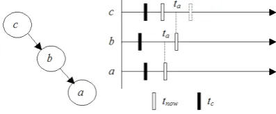
formula (such as Trapezoidal method) to (3), and solving the derived nonlinear algebraic equations by Newton’s iteration. The basic idea of BTWR is to consider the cause-and-consequence concept. The left part of Fig. 1 is a signal flow graph for partitioned subcircuits, in which the transient solution of subcircuit a is obviously the consequence of transient solutions of b and c. Therefore, b and c need to be solved before a to raise the computation efficiency. To trace these cause-and-consequence relations, we use the backward graph traversal technique. Introducing more clearly, we define some variables inside each subcircuit: tc is the time point for which the subcircuit has converged so far, tnow is the current time point to be solved, and ta (time arrived) is the time boundary at which the subcircuit is asked to be solved. In Fig. 1, the traversal starts from subcircuit a (tries to solve for y at a.tnow). The traversal visits a’s fan-in subcircuit b at first and ask it to be solved at time point later than b.ta (which is also a.tnow) in order to provide waveform references for subcircuit a. The traversal then continually visits c and asks it to be solved at time point later than c.ta (which is also b.tnow) for the same sake. Subcircuit c needs to forward two time points to move its tnow to over c.ta. In Fig. 1, the actual subcircuit calculation sequence would be: c be solved at its two tnow time points, b be solved at its tnow time points, and then a be solved at its tnow time points. This process might repeat several times until a.tnow is converged. The job of main program of BTWR is simple. It just picks subcircuit with smallest tnow, activates the “starting” backward traversal (called Mode-0 traversal) from it, and repeats the same process until no subcircuit left.
There are software schemes [3] to handle the feedback subcircuits (including adjacent coupling and global feedback loops) to strengthen the robustness of BTWR. BTWR exhibits several advantages. First, the multi-rate behaviors of circuits can be exploited. Second, the windowing technique [1] is automatically applied. Third, the function of selective-tracing scheme of ITA [2] (to calculate connected subcircuits) is retained. Finally and most important for this paper, it’s easy to implement high quality SOD on BTWR. BTWR is represented in pseudo codes of Algorithm 1. Note that SOD function is built in lines labeled by “Sod1” and “Sod2.”
Algorithm 1 (BTWR-based Circuit Simulation):
// ckt is the simulated circuit partitioned into N subcircuits. // Simulation duration is Tbegin∼Tend
BTWR(ckt, Tbegin, Tend) {
Set tc, tnow of all subcircuits to their initial values;
while(there is any subcircuit whose tc is not equal to Tend) {
Pick the subcircuit x with smallest tnow;
Sod1:
if(! contribute[x]) continue; // the SOD function
BTWRtrace(0, x.tnow, x); // begin to call the traversal
} }
BTWRtrace(mode, ta, sub) {
// sub.in_stack array records whether sub has been traversed
if(mode is 0) Clear all subcircuits’ in_stack flag, tever = 0;
else if(mode == 1) sub.in_stack = 1;
if(mode is 0) Clear GFL; // the set containing subcircuits of GFLs dtnow = sub.tnow; // the old tnow
do {
for(all sub’s fan-in subcircuit x) { // backwardly traverse all predecessors
if(x is strongly coupled with sub) synchronize x and sub; Rtr: if(! sub.in_stack) BTWRtrace(1, sub.tnow, x);
Loop: else { // has encountered a back edge
Add subcircuits from sub to x (in the recursion queue) into GFL;
}
}
S1: if(sub is not in GFL) { // simulate sub or all subcircuits in GFL
Solve (3) of sub at sub.tnow;
if(Newton iteration diverges or solution quality is bad) reduce tnow; // shrink the time step
else if(results have been converged) { tever = MAX(tever , sub.tc);
sub.tc = sub.tnow;
Estimate new sub.tnow;
}
}
S2: if(sub is the first subcircuit of GFL) { // simulate GFL Simulate GFL by using WR algorithm;
break;
}
Sod2: contribute[sub] = true; // the SOD function Stop1: if(mode is 0 && sub.tc >= dtnow) break;
Stop2: else if(mode is 1 && tever >= ta) break;
} while (true); }
B. ITA Algorithm
ITA [2] is a well-known algorithm, which belongs to relaxation-based class of algorithms and is frequently adopted as the algorithm of FAST SPICE programs. So, it’s valuable to discuss the parallel simulation of ITA. Its algorithm can be found in [2] and many other literatures. In this work, ITA is used to simulate both time and sensitivity simulations.
Fig. 1. A traversal starting from subcircuit a. Subcircuit b and c are asked to be calculated to time point later then ta.
As we explain earlier, SOD is to simulate the least number of subcircuits and still to satisfy users’ requirements. Processed by relaxation-based algorithm, the entire circuit has been partitioned into subcircuits that can be viewed as a directed graph called subcircuit signal flow graph (in which subcircuits are viewed as vertices, and affecting relations are viewed as directed edges). We can identify subcircuits having “contributions” to the user-wanted nodes by graph traversals. The method is to backwardly traverse the directed graph from nodes of interested, and mark all subcircuits traversed. In performing simulation, the unmarked subcircuits are just bypassed. Note that this method is simple and is based on the “static” subcircuit signal flow graph. If we want to use the “dynamic” subcircuit signal flow graph (which considers the conducting situations of transistors) that is more accurate, we should use BTWR.
C. Sensitivity Computation
others. So, the strategy to partition the sensitivity simulation task in CSM is clear: we just partition the list of design parameters. This CSM partition strategy can be called distribution by direct dividing, while the CSM partition strategy for BTWR and ITA can be called distribution by SOD. Note that in sensitivity computation, both these two partition strategies can be applied together. But in our sensitivity simulation program, only distribution by direct dividing is implemented.
III. THE COMBINING SIMULATION METHOD
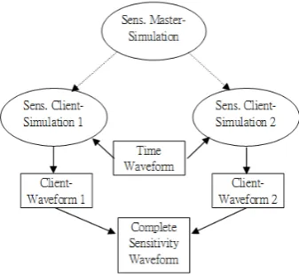
In using relaxation-based algorithm, there exist many strategies to utilize the parallelism. These strategies can be classified into space, temporal, and iteration respects [4]. The Combining Simulation Method belongs to the space respect. The basic idea is to use “client” processors to simulate different portions of the simulated circuit, and then combine the obtained “client-waveforms.” CSM using two processors is illustrated in Fig. 2. In this figure, there is a master-simulation that analyzes the simulated circuit, divides the circuit, sends the divided portions to client-simulations (which is simulated by one single processor), waits for the end of client-simulations, and then combines client-waveforms. The client-simulation just simulates given portion of the analyzed circuits and generates the sub-waveforms (client-waveforms). There might exist modifications for the basic scheme of Fig. 2. For example, the sensitivity case is shown in Fig. 3, in which the time waveform (in the center square) is pre-calculated to be used by all sensitivity client-simulations.
CSM is simple and is not applicable to all problems. The key factor for successfully utilizing CSM is that the considered simulation can be divided into independent portions. Once the considered simulation is certified to pass this criterion, it can be parallel processed by CSM. For the correctness and efficiency of CSM, dividing the simulated circuit is a critical step. The divided portions of the simulated circuit should be independent or the client-waveforms would be inaccurate. It is possible to undertake waveform relaxation between client-simulations to achieve the convergence of client-waveforms like [4], but we don’t consider this “complex” process in this paper. In this paper, we don’t really divide the simulated circuit. We use the mentioned distribution by SOD and distribution by direct dividing instead.
In using the distribution by SOD, we just divide the list of wanted outputs and send them to client-simulations, while each client-simulation simulates the same circuit. This strategy is simple and trustable, since each client-simulation simulates the entire circuit by using SOD, in which the obtained client-waveforms are accurate and no waveform relaxation processes are needed. To derive better efficiency of CSM, client-simulations have better to exhaust roughly the same amount of CPU time (which is for load balancing among processors) and simulate as few overlapping portions of the simulated circuit as possible. These necessities can be taken cared by well dividing the list of wanted outputs. The criterion for dividing outputs is to put outputs of the same independent portion of the simulated circuit together such
that they can be computed by the same client-simulation. Since SOD is used, the client-simulation will only simulate the related independent portion of the simulated circuit, and hence save the simulation time. To accomplish this dividing criterion, we need to analyze the simulated circuit. Because the
Fig. 2. An example of combining simulation method, in which only two processors (and hence two client simulations) exist.
Fig. 3. The example of applying combining simulation method in sensitivity computation, in which there are only two processors.
Relaxation-based algorithms (BTWR and ITA) are used, the simulated circuit has been partitioned into subcircuits. We can utilize the signal flow graph of subcircuits to do such analysis, e.g. traversing the signal flow graph from the wanted outputs backwardly to see the “contributing” subcircuits.
In dealing with sensitivity computation, the distribution by direct dividing is used. The design parameter list is divided equally into several smaller lists that are sent to client-simulations.
We have implemented CSM using BTWR and ITA for “time” simulation (circuit simulation), in which distribution by SOD is used for partitioning. Also, CSM using ITA for sensitivity simulation is implemented, and distribution by direct dividing is used for partitioning. Note that sensitivity client-simulations read time waveforms from files (time waveforms are needed for all sensitivity client-simulations) at the beginning of sensitivity computation.
There are overheads for reading and writing waveforms in using CSM. The amounts of overheads depend on the data size of time/sensitivity waveforms in Fig. 3 and Fig. 4. Such overhead is called “IO time” here, which will be recorded in our experiments. In using ITA, the points in time waveforms are usually dense [6]. This is due to that, in ITA, global time points are used for all subcircuits. Dense time points cause big waveform files. This problem can be alleviated by using the Multi-rate ITA [6]. Also, reducing time points of ITA waveforms can further reduce sizes of waveform files and hence to reduce the IO time.
IV. EXPERIMENTAL RESULTS
We have implemented all proposed methods in MOSTIME, and test them in multi-core PCs. When CSM is running, “master-MOSTIME” and several “client-MOSTIME” execute at the same time like Fig. 2. The master-MOSTIME activates client-MOSTIME and then combines client-waveforms, in which the passing of simulated circuits (which is described in “deck” files) and retrieving of client-waveforms all use the file system of Windows.
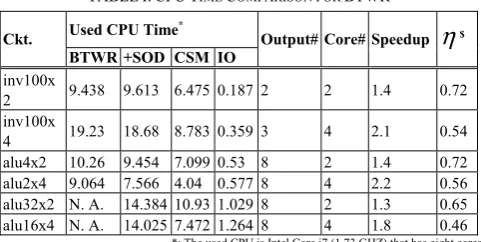
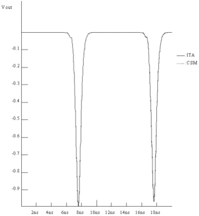
At first, we check the effect of BTWR-based circuit simulations. Several circuits have been simulated, and results are listed in Table I. The two types of circuits are inverter chain and ALU (whose schematic is given in Fig. 4) chain, both of which are composed of CMOS gates. Timing waveforms of the 4-bit ALU simulated by BTWR and CSM are compared in Fig. 5 and sensitivity waveforms of the 10-staged inverter chain simulated by ITA and CSM are compared in Fig. 6 respectively. The good waveform matches shows that implementations are correct. There are several independent portions in these circuits and they can be recognized by circuits’ names, e.g. “inv100x2” has two independent inverter chains. The number of cores is specified manually according to the number of independent portions. Numbers of outputs, which are important in SOD, are shown in Table 1, too. Three algorithms have been performed for each circuit, which are BTWR, BTWR plus SOD and BTWR-based CSM. The used CPU times of simulations are listed in columns. The column labeled with “IO” includes the time for writing client-waveforms (by client-simulation) and combining client-waveforms (by master-simulation), which can be referred to know the amount of overheads for processing client-waveforms. In the two right-most columns are speedup (compared with BTWR+SOD) and efficiency of CSM. Note that efficiency is defined as follows:
# * ) (
) (
Core CSM T
SOD BTWR
T +
=
η (4)
In which T(x) is the used CPU time of algorithm x. We can
observe obvious performance enhancements. Note that last two circuits have not simulated well by BTWR (and ITA) due to the reason of not enough memory. The efficiencies of parallel computing are not good in some circuits, e.g. in the last circuit, only 46% of efficiency is recorded. We find that one client-simulation, which needs to compete for “global resources” of the same PC (such as the right to access disc and main memory) with other client-simulations, spends more simulation time than normal simulation. In this respect, to use network of PCs is an improvement method.
ITA-based circuit simulations are then summarized in Table II. We firstly compare ITA and BTWR and find that BTWR performs better. This is due to that simulated circuits are all “one-way” circuits, so BTWR can converge well and simulate quickly (it can utilize multi-rate behaviors of circuits). Next, we check the speedup and parallel efficiency of CSM. The results are similar to those of BTWR. CSM using ITA works well, too. But, the IO time is much worse than those of BTWR. In our implementation, the waveform has been reduced (removing redundant time points) and IO time includes the time for this reduction. Obviously, in ITA-case the IO time is too big. However, we think we can solve this by selectively storing wanted waveforms rather than storing all waveforms (the implemented version).
Now we check the parallel sensitivity computations. There are 20 design parameters in each experiment of Table III, and there are two cores in the used computer. So, each client-simulation just simulates 10 design parameters. The used algorithm is ITA (which causes dense waveforms). We can find that the speedup and parallel efficiency are satisfactory. Due to the dense waveforms caused by ITA, the IO time can’t be omitted, too (which is not listed). We think it can be compensated in the case of dealing with more design parameters and using more processors.
V. CONCLUSION
In this paper, we have presented techniques to utilize the popular and powerful multi-core PC. These techniques are CSM, and circuit and sensitivity simulations based on CSM. Relaxation-based algorithms, BTWR and ITA, are utilized in CSM to calculate both time and sensitivity simulations. The complete implementation on multi-core PC has been tested. Experimental results justify that proposed techniques provide good parallel-computing efficiencies. Finding more complicated and better partitioning methods for CSM and applications for CSM are our future works.
TABLEI:CPUTIME COMPARISON FOR BTWR
Ckt. Used CPU Time* Output# Core# Speedup
η
$BTWR +SOD CSM IO
inv100x
2 9.438 9.613 6.475 0.187 2 2 1.4 0.72 inv100x
4 19.23 18.68 8.783 0.359 3 4 2.1 0.54 alu4x2 10.26 9.454 7.099 0.53 8 2 1.4 0.72 alu2x4 9.064 7.566 4.04 0.577 8 4 2.2 0.56 alu32x2 N. A. 14.384 10.93 1.029 8 2 1.3 0.65 alu16x4 N. A. 14.025 7.472 1.264 8 4 1.8 0.46
TABLEII:CPUTIME COMPARISON FOR ITA
Ckt. Used CPU Time* Output # Core # Speedup
η
ITA +SOD CSM IO
inv100x2 47.81 47.47 27.65 10.3 2 2 1.7 0.86
inv100x4 93.47 93.3 37.25 13.3 3 4 2.5 0.6 3
alu4x2 60.7 53.6 34.8 21.1 8 2 1.5 0.7 7
alu2x4 45.19 37.98 15.88 10.5 8 4 2.4 0.60
alu32x2$ N. A. 21.21 14.49 8.5 8 2 1.5 0.7 3
alu16x4$ N. A. 19.45 9.703 8.6 8 4 2.0 0.5 0
*: The used CPU is Intel Core i7 (1.73 GHZ) that has eight cores $: The used algorithm version is the so-called Multi-rate ITA [6]
TABLEIII:CPUTIME*COMPARISON FOR PARALLEL SENSITIVITY
SIMULATIONS$
Ckt. ITA CSM+ITA Core # Speedup
η
inv100x2 38.5 20.3 2 1.89 0.95
alu4x2 140.5 103 2 1.36 0.68
*: CPU is Intel Core 2 Duo (2.53 GHZ) that has two cores $: there are 20 design parameters (width of MOSFET) in each experiment
Fig. 4. The schematic of ALU.
Fig. 5. Waveform comparison for circuit alu4-2, which has two 4-bit ALU. The “CSM” means the “CSM+BTWR” algorithm.
Fig. 6. Sensitivity waveform comparison for 10-staged inverter chain,where design parameter is the width of the MOSFET in the first gate. The “CSM” means the “sensitivity CSM+ITA” algorithm.
REFERENCES
[1] A. R. Newton and A. L. S. Vincentelli, “Relaxation-based electrical simulation,” IEEE Trans on CAD, vol. CAD-3, pp. 308-311, Oct. 1984. [2] R. A. Saleh and A. R. Newton, “The exploitation of latency and multirate behavior using nonlinear relaxation for circuit simulation,”
IEEE Trans., Computer-aided Design, vol. 8, pp. 1286-1298,
December 1989.
[3] C. J. Chen, T. N. Yang, and J. D. Sun, “The Backward-traversing Relaxation Algorithm for Circuit Simulation,” IEEE Custom
Integrated Circuit Conference, San Jose, California, pp. 353-356,
September 10-13, 2006.
[4] C. P. Soto, R. Saleh, and T. Kwasniewski, “Time warping-waveform relaxation in a distributed circuit simulation environment,” pp. 338-341,
in Proceedings of the 38th Midwest Symposium on Circuit and System,
1995.
[5] C. J. Chen and W. S. Feng, “Transient sensitivity computations of MOSFET circuits using Iterated Timing Analysis and Selective-tracing Waveform Relaxation, in Proceeding of 31st Design Automation
Conference, pp. 581-585, San Diego CA, June 1994.
[6] C. Chen, C. C. Chang, C. J. Lee, C. L. Tsai, A. Y. Chang, and J. D. Sun, “The Multi-rate Iterated Timing Analysis Algorithm for Circuit Simulation,” 53rd IEEE International Midwest Symposium on Circuits
and Systems, Seattle USA, pp. 821-824, Aug. 1-4 2010.
Chun-Jung Chen received the B.S. degree in electrical engineering from National Taiwan University, Taipei, Taiwan, in 1989, and the Ph.D. degree in electrical engineering from National Taiwan University, Taipei, Taiwan, in 1994.
He is now an Associate Professor of the Department of Computer Science of Chinese Culture University in Taipei Taiwan. His research interests include circuit simulation, transient sensitivity computation, and parallel computing.