Partial diallel crosses for predicting yield of
semiexotic maize populations
C.M. Silva1, J.B. Miranda Filho2, U.C. Mendes3 and E.F. Reis1
1Programa de Pós-Graduação em Agronomia, Universidade Federal de Goiás,
Jataí, GO, Brasil
2Departamento de Genética, Escola Superior de Agricultura Luiz de Queiroz,
Universidade de São Paulo, Piracicaba, SP, Brasil
3Programa de Pós-Graduação em Agronomia, Universidade Estadual Paulista,
Campus Ilha Solteira, SP, Brasil
Corresponding author: E.F. Reis E-mail: [email protected]
Genet. Mol. Res. 16 (1): gmr16019544 Received November 21, 2016
Accepted January 23, 2017 Published February 8, 2017
DOI http://dx.doi.org/10.4238/gmr16019544
Copyright © 2017 The Authors. This is an open-access article distributed under the terms of the Creative Commons Attribution ShareAlike (CC BY-SA) 4.0 License.
plot after thinning. The following traits were analyzed: male flowering (days), stalk diameter (mm), plant height (m), ear height (m), tassel length (cm), tassel branch number, ear length (cm), ear diameter (cm), ear yield (t/ha), and grain yield (t/ha). The populations under study presented acceptable levels for yield potential and agronomic traits, thus assuring good perspectives for their use in breeding programs. The prediction for the new populations to be synthesized from the cross between the two groups of varieties contributed positively and HG-3 population was the most appropriate, in both eras, as the parent variety most promising in Group II (HG to be used as a base) for incorporation of varieties of Group I (NAP).
Key words: Diallel analysis; Genetical enhancement; Prediction of composites
INTRODUCTION
The maize crop has been recognized as one of the most important for the expansion of the Brazilian agriculture. In the last three decades, maize has been cultivated in two seasons of the same year: 1st crop (safra - October to January) and 2nd crop (safrinha - February to May), with planting date varying in different regions. The yield level of the 2nd crop (usually corn after soybean) has increased continuously during the last years and in some regions the cultivated area has been higher than the 1st crop. The Central West region represents more than 65% of the maize crop in the 2nd season in Brazil (CONAB, 2015). Besides the expansion of the maize crop in time it also has occurred extensively in space by opening new frontiers, thus increasing the variation of environments (latitude, altitude, fertility, biotic and non-biotic stresses, etc.). Such great changes justify the interest for new sources of germplasm to increase the chances of success of breeding programs to attend the new and expanding demands for adapted and outstanding genotypes.
The introduction of exotic germplasm in breeding programs has long been recognized as an important strategy to increase genetic variability and for incorporation of important genes not existing in the local varieties (Goodman, 1985; Nass et al., 2001). In Brazil, the great variability that characterize the maize germplasm has a significant contribution of exotic sources that largely contributed to increase the efficiency of breeding programs for the development of cultivars (Miranda Filho, 1992; Santos and Miranda Filho, 1992; Regitano Neto et al., 1997). Old local varieties such as Cateto and Dente Paulista were the first sources for the development of the hybrid seeds. The introduction of exotic germplasm, mainly Tuxpeño and related races of Mexico and Central America, largely contributed for the development of outstanding semident hybrids (Miranda Filho and Viégas, 1987). Later on, several other introductions were continuously accomplished (Moro et al., 1981; Nass et al., 2001). In spite of the cognizance on the role of previous introductions, recently there has been an increasing interest for new sources of germplasm, particularly focusing the resistance or tolerance to several kinds of stresses (Basso and Miranda Filho, 2001; Oliveira et al., 2015).
MATERIAL AND METHODS
Two groups (I and II) of open-pollinated populations (herein designated as varieties) were used in the present study based on crosses between groups, following the partial diallel scheme as given by Geraldi and Miranda Filho (1988).
Origin of Group I
The project named as Núcleo de Apoio à Pesquisa do Milho (NAP-MILHO) was coordinated by the Department of Genetics (ESALQ-USP, Piracicaba, SP, Brazil) and conducted in a cooperative system involving several public and private research institutions for the identification of sources of resistance for leaf diseases among accesses of the Brazilian Germplasm Bank of Maize (CENARGEN-EMBRAPA). The selection process led to the synthesis of five populations (composites) that were symbolized by NAP and related to specific foliar diseases, as follows: NAP-PP, NAP-PM, NAP-PZ, NAP-HT, and NAP-CS, representing resistance to Puccinia polysora, Phaeosphaeria maydis, Physopella zeae, Exerohilum turcicum, and corn stunt complex, respectively. Other four populations were later derived from the selected accesses after phenotypic selection for type of endosperm, and were designated as NAP-FA, NAP-FL, NAP-FB, and NAP-DB, with characteristics recognized as yellow flint, orange flint, white flint, and white dent, respectively. Therefore, the nine NAP populations comprised the Group I as already mentioned. More details about the origin of the NAP populations are given by Miranda Filho et al. (2000) and Mendes et al. (2015).
Origin of Group II
In the period covered by the years 2000 to 2004, several samples of commercial maize crops were collected in the field of local farmers within the region of the Southwest of Goiás State; such samples represented the F2 generations of maize hybrids with acceptable patterns of productivity, adaptation and important agronomic traits such as lodging resistance, plant architecture and tolerance to biotic and non-biotic stresses. The sampled populations were symbolized as HG and five of them were chosen to compose Group II of varieties used in the present study.
The two groups of populations (varieties) were identified by numbers as follows: Group I: [1. FA, 2. FL, 3. FB, 4. DB, 5. HT, 6. PP, 7. NAP-PZ, 8. NAP-PM, 9. NAP-CS]. Group II: [1’. HG-40, 2'. HG-54, 3'. HG-55, 4'. HG-75, 5'. HG-81]. The 14 parental varieties were multiplied by sib-cross within varieties and crossed according to the partial diallel (intergroup) as suggested by Geraldi and Miranda Filho (1988). Therefore, the whole set of entries (59) in the diallel scheme comprised 14 parental varieties and 45 hybrid crosses. The commercial hybrids SH4080 and BG7046 were used as checks in the 1st and 2nd crops, respectively.
where Yij is the plot expression of the ith treatment at the jth replication whose effects are
represented by ti (fixed) and bj (random); eij is the random error term for individual plots. In the analysis, the experimental unity was represented by plot totals (MF, EY, GY) or plot means (SD, PH, EH, TL, NB, EL, ED: means of five plants or ears per plot).
Analysis of the variance of the diallel table (parental varieties and crosses) was accomplished with plot means of four replications, using the model presented by Geraldi and Miranda Filho (1988). In such model, the effect of treatments is partitioned in three groups: Varieties I, Varieties II and hybrids (variety crosses), representing Group I, Group II and hybrids (Group I x Group II). The diallel itself is analyzed only with variety crosses and the appropriate model is an adaptation of Method-IV of Griffing (1956), as shown by Geraldi and Miranda Filho (1988):
where eij is the error term adjusted to means of r replications, or
µ is the mean of all crosses, gi and gj are the effects of general combining ability (GCA) of varieties in Group I and Group II and sij is the effect of specific combining ability (SCA); except for eij, all other effects are fixed. An alternative model for the analysis of the diallel
table should be the model for partial diallel suggested by Miranda Filho and Geraldi (1984), that is based on the heterosis and its components, as an adaptation to the model of Gardner and Eberhart (1966); however, for the purpose of the present study the model discussed by Geraldi and Miranda Filho (1988) was considered the most appropriate.
As already mentioned, the main purpose of the present study was to obtain information about important quantitative characters in two distinct groups of populations (herein designated as varieties) and their use for guiding the synthesis of new populations for breeding objectives.
The methodology for prediction of population means was used for the identification of two types of populations: a) Population resulting from the recombination of the variety cross (NAP x HG = Group I x Group II), for the identification of the local population (HG from Group II) most promising for the incorporation of each semiexotic population from Group I. b) Hybrid combinations (NAP x HG) most appropriate for the exploitation of heterosis at the interpopulation level, also looking forward to the development of inbred lines to be used in hybrid crosses.
In (a) it was used the prediction formula given by Miranda Filho (1974) and Hallauer and Miranda Filho (1988):
where ϕ is the expected mean of the composite formed with 50% of one semiexotic variety (Equation 1)
ij
i
j
ij
Y
= + + +
µ
t b e
ij i j ij ij
Y
= + +
µ
g g s e
+ +
(Equation 2)(Equation 3)
/
ij j ij
e
= Σ
e r
(Equation 4)
0 0
1( ) 1 1
2 Y Yv 2h n4n hv
(NAP, Group I) and 50% of varieties of Group II (HG), used as basic material for incorporation;
0
Y is the observed mean of the semiexotic population; YV is the mean of k varieties used as the
base for incorporation; h0 is the average heterosis of crosses between the semiexotic variety
and the k varieties of Group II; hV is the average heterosis of crosses between the k varieties. In the present study, only one variety HG will be used for incorporation of each NAP, so that k = 1, hV does not exist and the prediction formula and is reduced to
which is equivalent to the formula of Mather and Jinks (1982) for prediction of the F2 generation from the cross between two inbred parents. In the present case, the resulting population is a composite of size s = 2, obtained by recombination of the F1 hybrid between two varieties. Since the recombination is a random procedure, the newly formed composite will be in Hardy-Weinberg equilibrium and literally ready to initiate a recurrent selection program.
In the scheme (b), the interest is on the hybrid between two composites, one from each group (I and II). For that purpose, selection of the basic germplasm was done in two distinct phases:
(b1) - Selection of the most promising varieties based on the effects of GCA in each group (gi in Group I and gj in Group II), estimated according to the model for partial diallel shown by Geraldi and Miranda Filho (1988); thus, only the varieties with positive estimates of gi and gj were chosen for predicting means, as planned. Finally, the following sets of varieties were chosen: (3, 6, 7, 8) in Group I and (4', 5') in Group II, under the conditions of 1st crop; and (1, 6, 7, 8) and (3', 5') under the conditions of 2nd crop, respectively.
(b2) - Predicting means of hybrids between composites of different groups. With the n1 varieties taken from Group I, nр1 = 2n1 - 1 populations (combinations) will be available, including
the n1 varieties plus 2n1 - (n
1 + 1) composites of size k ≥ 2; for n1 = 4, it follows nр1 = 15. In Group
II, it will be available nр2 = 3 (two varieties and the composite of size s = 2). Therefore, the possible number of hybrids between composites will be Nc = nр1 . nр2 = 45. The same calculation holds for both 1st and 2nd crops because the same number of available varieties. The predicted mean of the hybrid between composites (composite I x composite II) is given by
where fi is the proportion that each variety of Group I (Vi) enter in the composite; the same thought applies to varieties of Group II (Vj). Actually, the formula above is symbolic and if expressed algebraically would be
which still is a conceptual definition, that to be an effective formula the product ViVj must be replaced by the observed mean of the hybrid Hij; then, the effective formula for prediction of the cross between two composites (Eberhart et al., 1967; Vencovsky and Barriga, 1992) is
(Equation 5)
0 0
1
(
)
1
2
Y Y
v2
h
ϕ
=
+
+
(Equation 6)
1 2
k i i k j j
i j
x f V f V
ϕ
ϕ
Ι ΙΙ=
∑
∑
(Equation 7)
x
i j i j i j,
f f VV
In the present case, the representation of the genetic source within brackets may include only one variety with frequency fi = 1, as in the example [V1] x [1 1
1´ 2´
2V +2V ], which would result in
the hybrid with mean predicted by 1
2(H11’ + H12’).
In the present study, with previous selection of varieties based on estimates of GCA, the prediction process reduces to 45 crosses, as already shown. Nevertheless, the prediction of all possible hybrids comprising the whole set of varieties (9 in Group I and 5 in Group II) would lead that number to (29-1) (25-1) = 15,841.
RESULTS AND DISCUSSION
Means and variances
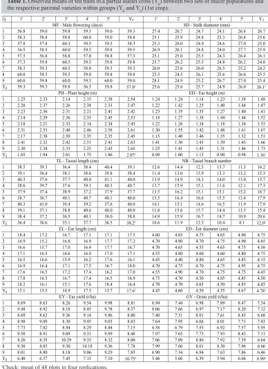
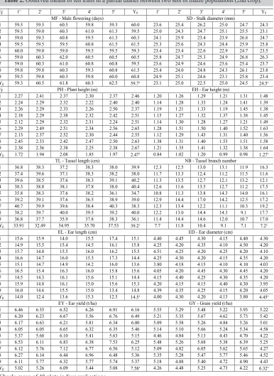
The observed means of ten plant and ear traits are shown in Tables 1 and 2 referring to two planting seasons (1st crop - e1: safra; 2nd crop - e2: safrinha, respectively); the whole set of means includes nine varieties of Group I, five varieties of Group II and 45 hybrid crosses (Group I x Group II). Means for each trait in experiments of two seasons are summarized in Table 3.
For male flowering, practically there was no difference among groups (Varieties I, Varieties II, Hybrids) with means around 59 days in ε1 and around 60 days in ε2. However, the earliest (lower mean) in ε1 was for 5 (NAP-HT) in Group 1, 4’ (HG-75) in Group II and the hybrid 4 x 1’ (NAP-DB x HG-40); in ε2 the earliest varieties were the same as in ε1 and the hybrid crosses were very similar (around 60 days). It was concluded that expression of male flowering for both groups of parent varieties and hybrids was within the pattern of cultivars of maize commonly in use. Souza (2015) reported male flowering (days) as 60.9, 63.1 and 61.7 in the semi-exotic populations CRE-01, CRE-02, and CRE-03, which were higher than the check hybrids (P30K75 and SHS 4080) by 4.2, 6.0, and 4.8%, respectively.
SD also showed to be very similar among groups, in the range of 24 to 26 mm in the whole set. The only difference was that means were a little lower for all groups (less than 1.1 mm on average) in ε2. The same pattern of expression among groups in two seasons was observed for plant height and ear height. However, it was possible to identify 3 (NAP-FB) and 4' (HG-75) as the smaller means for plant height in e1 and 3 and 1' (HG-40) in ε2. The lower means for ear height were exhibited by the same parental varieties as for plant height in both seasons.
TL and NB, on the average for each group, were in the range of 34 to 40 and 9 to 18, respectively; for both traits there was a slight decrease from ε1 to ε2. Such ranges were somewhat below the ranges (36.1 to 46.0 and 12.6 to 23.8, averaging 40.9 and 18.4, respectively) reported by Andrade and Miranda Filho (2008) for half-sib family means of the maize population, ESALQ-PB1. Souza (2015) reported means for TL and NB, around 38 and 14 in three semi-exotic populations (CRE-01, CRE-02, CRE-03). For both TL and NB, as a measure of tassel size, Group I showed a slightly higher mean than Group II in both seasons, which is a coherent result, because modern germplasm derived from commercial cultivars, as is the case of varieties of Group II, tends to exhibit smaller tassels.
EL and ED showed a similar pattern of expression as for TL and NB in the three groups, i.e., Group II < Hybrids < Group I in ε1 and Group II < Group I < Hybrids in ε2. In general, there was a decrease in means from ε1 to ε2 in both traits.
(Equation 8)
,
i j i j ij
x
f f H
Table 1. Observed means of ten traits in a partial diallel cross (Yij) between two sets of maize populations and the respective parental varieties within groups (Yij and Yij) (1st crop).
i\j 1' 2' 3' 4' 5' Yii 1' 2' 3' 4' 5' Yii
MF - Male flowering (days) SD - Stalk diameter (mm)
1 56.8 59.0 59.8 59.3 59.0 59.3 27.4 26.7 24.7 24.1 26.8 26.7
2 58.3 58.8 59.8 60.0 59.0 58.8 25.1 25.9 24.8 25.3 26.8 25.6
3 57.8 57.8 60.3 59.5 59.5 58.3 25.3 26.0 24.9 24.6 27.0 25.0
4 56.5 58.5 60.0 59.5 59.8 59.5 26.9 26.1 24.8 24.0 27.7 25.9
5 57.5 56.8 58.8 57.0 58.8 57.3 25.1 25.0 25.5 24.3 26.4 26.1
6 57.3 59.8 60.5 59.3 59.8 59.8 25.7 26.2 25.5 24.8 26.2 24.8
7 58.3 59.3 60.5 58.0 59.3 59.3 26.0 25.6 26.0 26.5 25.2 24.2
8 60.0 59.3 59.5 59.0 59.8 59.8 25.5 24.5 26.1 25.6 26.6 25.5
9 60.0 59.8 60.0 59.3 60.0 59.0 28.1 24.9 25.2 26.7 27.0 25.4
Yjj 59.3 59.3 59.8 56.5 59.8 57.0 25.6 25.6 25.7 24.9 26.0 26.1
PH - Plant height (m) EH - Ear height (m)
1 2.25 2.33 2.14 2.15 2.38 2.54 1.24 1.24 1.14 1.23 1.38 1.48
2 2.20 2.37 2.26 2.38 2.33 2.47 1.22 1.42 1.25 1.40 1.44 1.47
3 2.23 2.36 2.31 2.21 2.41 2.42 1.23 1.35 1.35 1.27 1.40 1.41
4 2.14 2.29 2.36 2.35 2.45 2.53 1.18 1.27 1.38 1.44 1.44 1.52
5 2.18 2.21 2.32 2.14 2.34 2.45 1.22 1.26 1.34 1.18 1.34 1.53
6 2.31 2.53 2.40 2.46 2.58 2.61 1.30 1.55 1.42 1.48 1.61 1.67
7 2.17 2.38 2.50 2.35 2.35 2.45 1.15 1.40 1.46 1.35 1.32 1.51
8 2.41 2.32 2.42 2.51 2.41 2.63 1.41 1.30 1.43 1.59 1.45 1.66
9 2.30 2.34 2.33 2.25 2.45 2.65 1.25 1.41 1.43 1.31 1.46 1.73
Yjj 1.85 1.94 2.01 1.75 1.86 2.07 0.99 1.00 1.13 0.90 0.98 1.16
TL - Tassel length (cm) NB - Tassel branch number
1 38.5 39.3 36.4 38.4 40.4 39.1 12.6 14.4 12.5 13.7 11.3 16.2
2 39.1 36.4 38.1 38.6 39.8 38.4 11.4 13.0 13.9 13.3 13.2 15.3
3 40.3 37.6 37.7 40.4 41.1 40.0 13.9 14.9 14.3 14.0 13.0 15.7
4 38.6 39.7 37.6 39.1 40.3 40.7 13.7 15.9 15.1 11.6 12.1 17.3
5 37.9 37.4 38.9 37.2 37.9 37.7 13.5 16.2 15.1 15.1 15.2 18.7
6 38.7 36.7 40.1 40.7 40.1 40.0 13.5 16.4 16.6 15.5 13.4 17.9
7 40.3 41.0 39.4 39.2 37.6 40.0 14.1 15.1 14.6 16.5 11.9 17.9
8 39.1 37.1 38.8 40.6 40.0 40.0 11.8 15.6 15.7 14.4 13.5 15.4
9 38.4 37.2 36.5 40.1 38.0 38.8 14.9 15.9 16.7 14.7 10.9 20.6
Yjj 36.4 36.6 35.1 37.7 36.5 38.2 10.6 11.9 12.3 10.4 8.1 12.0
EL - Ear length (cm) ED - Ear diameter (cm)
1 18.4 17.2 16.7 17.1 17.1 17.5 4.80 4.85 4.75 4.65 4.90 4.75
2 16.9 15.2 16.8 16.9 17.7 17.2 4.70 4.80 4.70 4.75 4.90 4.65
3 16.6 15.7 17.0 16.4 17.7 16.7 4.70 4.65 4.55 4.65 4.75 4.50
4 17.1 16.5 16.6 16.8 17.0 17.1 4.55 4.80 4.60 4.60 4.80 4.75
5 16.5 16.6 15.9 16.2 17.6 16.1 4.45 4.40 4.80 4.65 4.85 4.15
6 16.9 16.4 17.1 17.5 16.7 18.0 4.70 4.75 4.70 4.75 4.95 4.75
7 17.6 16.5 17.2 17.4 16.2 17.0 4.55 4.90 4.70 4.75 4.75 4.45
8 17.8 16.5 16.7 17.4 16.5 16.9 4.75 4.70 4.50 4.85 4.85 4.50
9 18.2 16.1 15.1 17.6 18.4 16.4 4.70 4.70 4.65 4.50 4.85 4.45
Yjj 15.1 15.5 14.9 17.5 13.7 17.6 4.45 4.60 4.50 4.55 4.67 4.78
EY - Ear yield (t/ha) GY - Grain yield (t/ha)
1 8.69 8.63 8.26 9.54 9.98 8.81 6.94 7.44 6.98 7.89 8.47 7.34
2 9.48 8.92 8.18 8.45 9.78 8.37 8.06 7.66 6.97 7.17 8.20 7.12
3 8.69 8.62 9.36 9.14 9.86 8.00 7.40 7.31 8.01 7.61 8.43 6.68
4 8.98 9.09 8.30 9.45 9.03 8.83 7.64 7.95 6.66 8.01 7.71 7.43
5 7.73 7.82 8.94 8.29 8.84 7.15 6.58 6.79 7.55 6.92 7.57 5.95
6 9.50 8.91 9.09 9.31 9.99 8.48 7.97 7.65 7.73 7.93 8.43 7.11
7 8.26 8.35 10.29 9.35 8.32 8.00 7.06 7.09 8.86 7.92 7.39 6.64
8 9.30 8.85 9.30 10.18 9.36 7.78 7.99 7.60 8.01 8.30 7.96 6.66
9 8.01 8.80 8.18 9.06 9.29 7.85 6.90 7.34 6.94 7.63 7.86 6.46
Yjj 6.40 6.57 7.45 7.15 7.10 10.75 5.46 5.60 6.39 5.94 6.04 8.99
Table 2. Observed means of ten traits in a partial diallel between two sets of maize populations (2nd crop).
i\j 1' 2' 3' 4' 5' Yii 1' 2' 3' 4' 5' Yii
MF - Male flowering (days) SD - Stalk diameter (mm)
1 59.5 59.5 60.5 59.8 59.3 60.0 23.6 25.4 26.2 25.0 24.7 24.3
2 59.5 59.0 60.3 61.0 61.3 59.5 25.0 24.3 24.7 25.1 25.5 23.1
3 59.0 59.3 60.8 59.5 61.3 60.3 24.1 25.9 23.4 23.9 26.8 24.7
4 59.5 59.5 59.5 60.8 61.5 61.5 25.3 25.6 24.3 24.4 25.9 25.8
5 60.0 59.0 59.0 59.5 59.5 59.3 23.4 23.4 22.6 22.9 24.7 23.5
6 59.0 60.3 62.0 60.5 60.5 60.5 25.8 24.7 25.3 24.9 26.8 26.3
7 59.0 60.3 61.0 60.8 60.8 59.5 23.6 24.9 24.6 23.6 25.4 23.7
8 59.8 59.8 60.3 59.3 60.8 61.5 25.4 24.0 24.8 24.3 26.1 23.8
9 59.5 59.8 60.3 59.8 60.0 60.8 24.9 25.1 24.6 23.1 25.8 23.4
Yjj 59.3 60.5 61.8 60.3 62.5 59.7 23.1 25.0 22.5 25.0 24.5 24.5
i\j PH - Plant height (m) EH - Ear height (m)
1 2.27 2.41 2.37 2.30 2.37 2.46 1.20 1.26 1.29 1.21 1.31 1.48
2 2.24 2.29 2.32 2.22 2.40 2.40 1.14 1.28 1.33 1.24 1.41 1.39
3 2.26 2.29 2.33 2.26 2.50 2.37 1.19 1.21 1.33 1.19 1.45 1.38
4 2.18 2.29 2.38 2.32 2.42 2.51 1.15 1.27 1.32 1.37 1.38 1.45
5 2.12 2.29 2.32 2.31 2.24 2.51 1.14 1.30 1.28 1.27 1.21 1.49
6 2.29 2.49 2.51 2.34 2.56 2.65 1.28 1.51 1.50 1.40 1.52 1.63
7 2.13 2.37 2.52 2.30 2.44 2.55 1.12 1.29 1.43 1.31 1.40 1.56
8 2.45 2.33 2.42 2.47 2.50 2.63 1.38 1.31 1.40 1.53 1.51 1.58
9 2.38 2.36 2.38 2.25 2.38 2.67 1.21 1.35 1.41 1.32 1.38 1.64
Yjj 1.72 1.94 2.08 1.85 1.97 2.47 0.84 1.02 1.20 0.99 0.98 1.27
TL - Tassel length (cm) NB - Tassel branch number
1 36.8 38.3 37.2 38.3 38.0 39.9 12.3 12.5 13.0 13.1 11.9 16.3
2 37.4 39.6 37.1 38.3 38.2 38.0 11.7 13.3 12.4 11.2 11.5 11.6
3 39.6 38.5 37.6 38.3 39.1 40.2 11.3 13.5 12.7 12.1 13.2 12.1
4 38.3 38.8 38.1 37.8 38.0 40.4 12.6 11.6 13.5 12.7 11.2 17.5
5 35.8 38.3 37.6 38.2 36.1 34.7 10.8 11.3 13.8 14.3 14.0 16.1
6 39.2 39.1 37.6 36.5 38.9 39.0 12.9 14.4 17.0 14.2 12.5 17.2
7 40.7 39.9 39.6 38.4 40.3 38.3 12.3 13.4 12.2 11.1 10.3 19.2
8 38.2 39.7 40.0 39.5 39.2 40.0 12.2 13.0 14.4 14.3 9.1 17.7
9 36.8 37.7 35.9 37.8 38.3 36.1 11.4 14.4 14.6 12.0 10.7 17.0
Yjj 33.91 32.49 34.95 35.70 37.53 39.2 7.7 11.8 10.4 9.1 7.1 7.2
EL - Ear length (cm) ED - Ear diameter (cm)
1 15.6 15.9 14.0 15.5 17.4 15.1 4.40 4.45 4.30 4.15 4.40 4.30
2 14.9 15.5 15.4 14.5 16.1 15.8 4.25 4.20 4.35 4.10 4.50 4.20
3 15.7 14.8 15.5 16.0 16.2 15.5 4.51 4.25 4.20 4.25 4.20 4.10
4 16.6 14.7 16.0 15.3 17.3 14.4 4.25 4.30 4.20 4.15 4.35 4.20
5 15.1 14.7 14.9 14.2 16.0 13.6 3.80 4.18 4.15 4.10 4.10 4.03
6 16.5 15.4 16.3 16.0 15.8 15.6 4.05 4.20 4.45 4.30 4.45 4.20
7 14.5 14.3 16.1 15.6 15.1 14.4 4.15 4.40 4.25 4.30 4.35 4.20
8 15.9 14.8 16.1 15.0 15.6 15.3 4.20 4.15 4.15 4.40 4.30 3.95
9 16.0 14.6 15.5 15.0 13.4 14.8 4.39 4.35 4.25 4.15 4.20 4.05
Yjj 14.0 12.4 13.6 15.3 12.5 14.5 4.00 4.30 4.20 4.13 3.80 4.45
EY - Ear yield (t/ha) GY - Grain yield (t/ha)
1 6.46 6.35 6.52 6.26 6.91 6.16 5.55 5.29 5.48 5.22 5.93 5.22
2 6.20 6.23 6.67 5.56 6.76 6.49 5.21 5.35 5.67 4.62 5.73 5.42
3 6.17 6.63 6.21 5.81 6.34 6.00 5.09 5.58 5.26 4.84 5.26 5.01
4 6.05 6.05 6.65 6.32 6.35 5.46 5.14 5.10 5.66 5.24 5.34 4.58
5 5.37 5.68 6.10 5.41 5.63 5.15 4.46 4.84 5.13 4.43 4.70 4.22
6 6.53 6.11 6.83 6.38 7.53 6.25 5.48 5.26 5.68 5.38 6.39 5.25
7 6.12 5.76 7.12 6.77 6.56 5.12 5.09 4.82 6.05 5.62 5.65 4.27
8 6.27 6.14 6.44 6.96 6.48 5.36 5.35 5.28 5.47 5.77 5.46 4.52
9 6.11 5.77 6.32 5.77 5.74 5.37 5.18 4.88 5.40 4.72 4.90 4.43
Yjj 5.02 5.26 6.09 5.44 5.08 7.58 4.26 4.48 5.25 4.73 4.22 6.32
1Seasons: ε
1 (1st crop = safra) and ε2 (2nd crop = safrinha). 2Diallel: refers to the whole set (Varieties I, Varieties II
and Hybrids). For abbreviations, see Tables 1 or 2.
Table 3. Observed means of ten traits in partial diallel cross (9 x 5) in two planting seasons (ε1, ε2)1.
Varieties I Varieties II Hybrids Diallel2
1 2 1 2 1 2 1 2
MF 58.97 60.31 58.90 60.85 59.01 60.00 59.00 60.12
SD 25.48 24.29 25.55 24.00 25.75 24.74 25.70 24.61
PH 2.527 2.527 1.880 1.911 2.329 2.346 2.321 2.337
EH 1.554 1.511 1.000 1.004 1.348 1.316 1.350 1.320
TL 39.40 38.51 36.46 34.91 38.80 38.28 38.70 38.03
NB 17.24 16.06 10.68 9.21 14.09 12.60 14.28 12.84
EL 16.97 14.93 15.32 13.55 16.87 15.43 16.75 15.19
ED 4.550 4.136 4.553 4.085 4.714 4.256 4.676 4.223
EY 8.140 5.706 6.932 5.376 8.973 6.275 8.673 6.112
GY 6.821 4.769 5.884 4.589 7.610 5.287 7344 5.149
The relatively lower expression of EL and ED in Group II is explained because this group was developed from recombination of commercial hybrids and this procedure leads to a decrease in the level of heterozygosity and consequently in the hybrid vigor (6.40% for EL and 3.56% for ED, on the average of two seasons; see Table 4). Comparing the sets (Group I, Group II, Hybrids), the highest means (cm) for EL were (18.0, 17.5, 18.4) in ε1 and (15.8, 15.3, 17.4) in ε2; for ED were (4.75, 4.67, 4.95) in ε1 and (4.30, 4.30, 4.51) in ε2. In the group of hybrids, the highest means for EL were in the crosses 9 x 5' (NAP-CS x HG-81]) and 1 x 5' (NAP-FA x HG-81); and for ED were in the crosses 6 x 5' (NAP-PP x HG-81) and 3 x 1' (NAP-FB x HG-40).
For abbreviations, see Tables 1 or 2. Seasons: e1 - 1st crop = safra, e2 - 2nd crop = safrinha.
Table 4. Average heterosis (h) for ten traits in a partial diallel cross between two groups of varieties evaluated
in two planting seasons (ε1,ε2).
Traits Season 1 Season 2 Traits Season 1 Season 2
h h% h h% h h% h h%
MF 0.075 0.13 -0.578 -0.95 NB 0.131 0.94 -0.036 -0.29
SD 0.241 0.94 0.594 2.46 EL 0.719 4.46 1.190 8.36
PH 0.126 5.72 0.127 5.70 ED 0.163 3.58 0.146 3.54
EH 0.071 5.57 0.059 4.70 EY 1.437 19.06 0.734 13.25
TL 0.877 2.31 1.566 4.26 GY 1.262 19.80 0.609 13.00
In season e1, the highest yielding varieties (ear yield and grain yield) were 1 (NAP-FA) and 4 (NAP-DB) in Group I, 3' (HG-55) in Group II and the hybrid 7 x 3' (NAP-PZ x HG-55). In season e2, the outstanding materials were 2 (NAP-FL), 3' (HG-55) and 6 x 3' (NAP-PP x HG-55), respectively. On average, Group I showed ear yield 17.4 and 6.1% higher than Group II in e1 and e2, respectively; for grain yield the corresponding values were 15.9 and 3.9%.
The average heterosis (h) expressed in variety crosses were below 5% (relative to
midparent) in most instances (Table 4); for plant traits h > 5% were detected only for PH in
Table 5. Heterosis (hij) for grain yield (t/ha) of hybrids (Hij) in a partial diallel evaluated in two planting seasons.
Hij hij hij% Hij hij hij% Hij hij hij% Hij hij hij%
Season 1
H11' 0.539 8.4 H33´ 1.468 22.5 H55' 1.581 26.4 H82' 1.470 24.0
H12' 0.969 15.0 H34´ 1.302 20.7 H61' 1.691 26.9 H83' 1.482 22.7
H13' 0.110 1.6 H35´ 2.067 32.5 H62' 1.298 20.4 H84' 2.006 31.9
H14' 1.256 18.9 H41´ 1.198 18.6 H63' 0.976 14.5 H85' 1.616 25.5
H15' 1.785 26.7 H42´ 1.432 22.0 H64' 1.406 21.5 H91' 0.942 15.8
H21' 1.768 28.1 H43´ -0.251 -3.6 H65' 1.853 28.2 H92' 1.312 21.8
H22' 1.302 20.5 H44´ 1.322 19.8 H71' 1.017 16.8 H93' 0.515 8.0
H23' 0.208 3.1 H45´ 0.978 14.5 H72' 0.975 15.9 H94' 1.426 23.0
H24' 0.637 9.8 H51´ 0.874 15.3 H73' 2.348 36.0 H95' 1.610 25.8
H25' 1.620 24.6 H52´ 1.016 17.6 H74' 1.636 26.0 Mean 1.258 19.8
H31' 1.332 22.0 H53´ 1.383 22.4 H75' 1.049 16.5 Max 2.348 36.0
H32' 1.174 19.1 H54´ 0.974 16.4 H81' 1.936 32.0 Min -0.251 -3.6
Season 2
H11' 0.803 16.9 H33´ 0.122 2.4 H55' 0.479 11.4 H82' 0.774 17.2
H12' 0.437 9.0 H34´ -0.038 -0.8 H61' 0.720 15.1 H83' 0.584 11.9
H13' 0.245 4.7 H35´ 0.646 14.0 H62' 0.390 8.0 H84' 1.139 24.6
H14' 0.248 5.0 H41´ 0.723 16.4 H63' 0.428 8.2 H85' 1.085 24.8
H15' 1.212 25.7 H42´ 0.566 12.5 H64' 0.391 7.8 H91' 0.831 19.2
H21' 0.372 7.7 H43´ 0.748 15.2 H65' 1.658 35.0 H92' 0.427 9.6
H22' 0.401 8.1 H44´ 0.588 12.6 H71' 0.826 19.4 H93' 0.555 11.5
H23' 0.335 6.3 H45´ 0.939 21.4 H72' 0.443 10.1 H94' 0.141 3.1
H24' -0.456 -9.0 H51´ 0.218 5.2 H73' 1.287 27.0 H95' 0.575 13.3
H25' 0.913 18.9 H52´ 0.486 11.2 H74' 1.122 24.9 Mean 0.609 13.0
H31' 0.456 9.8 H53´ 0.400 8.5 H75' 1.407 33.2 Max 1.658 35.0
H32' 0.835 17.6 H54´ -0.045 -1.0 H81' 0.960 21.9 Min -0.456 -9.0
For abbreviations, see Tables 1 or 2. aSources of variation: Replications, Populations and Error with 3, 58 and 174
degrees of freedom. PH, EH, ED, EY, and GY: mean squares multiplied by 102. CV = coefficient of variation.
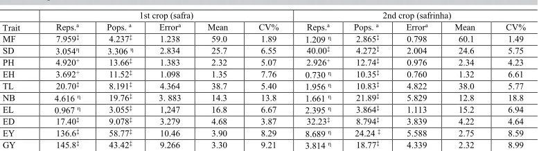
Table 6. Preliminary analysis of variance of ten traits in a partial diallel between two groups of varieties in
two crop seasons.
1st crop (safra) 2nd crop (safrinha)
rait Reps.a Pops. a Errora Mean CV% Reps.a Pops. a Errora Mean CV%
MF 7.959‡ 4.237‡ 1.238 59.0 1.89 1.209 2.865‡ 0.798 60.1 1.49
SD 3.054 3.306 2.834 25.7 6.55 40.00‡ 4.272‡ 2.004 24.6 5.75
PH 4.920+ 13.66‡ 1.383 2.32 5.07 2.926+ 12.74‡ 0.976 2.34 4.23
EH 3.692+ 11.52‡ 1.098 1.35 7.76 0.730 10.35‡ 0.760 1.32 6.61
TL 20.70‡ 8.191‡ 4.364 38.7 5.40 1.956 10.83‡ 4.822 38.0 5.77
NB 4.616 19.76‡ 3. 883 14.3 13.8 1.661 21.89‡ 5.829 12.8 18.8
EL 0.967 3.055‡ 1,247 16.8 6.67 2.395 3.864‡ 1.113 15.2 6.94
ED 17.40‡ 9.078‡ 3.279 4.68 3.87 32.23‡ 8.794‡ 3.839 4.22 4.64
EY 136.6‡ 58.77‡ 10.46 3.90 8.29 8.689 24.24 ‡ 5.588 2.75 8.59
GY 145.8‡ 43.42‡ 9.266 3.30 9.21 3.814 18.77‡ 4.339 2.32 8.99
aMean squares multiplied by 102 in MF, SD and TL; and by 103 in PH and EH. bAnalysis with means of four
replications in randomized blocks. For abbreviations, see Tables 1 or 2. ‡,+,hSignificance by F-test: P < 0.01, P < 0.05
and no significance, respectively. Contrasts: ѵ Y YI− II = ; Һ = YH - YV (See Material and Methods).
Table 7. Mean squaresa in the analysis of varianceb of five traits in a partial diallel between two groups of
varieties (1st crop).
Source d.f. MF SD PH EH TL
Populations 58 105.9‡ 82.64 34.15‡ 28.81‡ 20.48‡
Hybrids (H) 44 110.8‡ 95.18 11.83‡ 12.85‡ 17.67+
GCA-I 8 165.9‡ 48.50 24.39‡ 27.12‡ 18.11
GCA-II 4 443.6‡ 361.7‡ 33.45‡ 38.40‡ 39.78‡
SCA 32 55.41‡ 73.54 5.990+ 6.088‡ 14.80
Varieties I 8 64.76+ 58.87 7.550+ 11.75‡ 9.324
Varieties II 4 186.3‡ 16.53 9.638+ 6.704+ 8.759
Groups 2 3.072 34.02 680.5‡ 492.5‡ 150.2‡
Contrast (ѵ) 1 1.677 1.373 1349‡ 984.3‡ 278.2‡
Contrast (Һ) 1 4.467 66.68 11.92 0.676 22.27
Error 174 30.94 70.86 3.458 2.746 10.91
aMean squares multiplied by 10 in NB and EL; by 102 in EY and GY; and by 103 in ED. bAnalysis with means of
four replications in randomized blocks. For abbreviations, see Tables 1 or 2. ‡,+,hSignificance by F-test: P < 0.01, P <
0.05 and no significance, respectively. Contrasts: ѵ = YI - YII ; Һ = YH - YV (See Material and Methods).
Table 8. Mean squaresa in the analysis of varianceb of five traits in a partial diallel between two groups of
varieties (1st crop).
Source d.f. NB EL ED EY GY
Populations 58 49.40‡ 7.637‡ 22.69‡ 14.69‡ 10.86‡
Hybrids (H) 44 24.05‡ 5.136+ 15.64‡ 7.939‡ 5.724‡
GCA-I 8 31.87‡ 2.566 16.01 11.05‡ 7.903‡
GCA-II 4 106.3‡ 17.24‡ 54.81‡ 17.23‡ 11.52‡
SCA 32 11.81 4.265 10.65 5.999‡ 4.455‡
Varieties I 8 30.79‡ 3.226 39.37‡ 5.866+ 4.521
Varieties II 4 27.02+ 19.61‡ 7.139 3.849 2.805
Groups 2 726.3‡ 56.35‡ 142.3‡ 220.3‡ 165.2‡
Contrast (ѵ) 1 1383‡ 87.74‡ 0.036 94.99‡ 57.05‡
Contrast (Һ) 1 69.41‡ 24.95‡ 284.6‡ 345.5‡ 273.3‡
aMean squares multiplied by 102 in MF, SD and TL; and by 103 in PH and EH. bAnalysis with means of four
replications in randomized blocks. For abbreviations, see Tables 1 or2. ‡,+,hSignificance by F-test: P < 0.01, P < 0.05
and no significance, respectively. Contrasts: ѵ = YI - YII ; Һ = YH - YV (See Material and Methods).
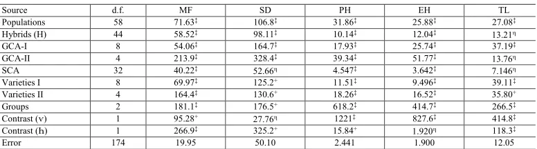
Table 9. Mean squaresa in the analysis of varianceb of five traits in a partial diallel between two groups of
varieties (2nd crop).
Source d.f. MF SD PH EH TL
Populations 58 71.63‡ 106.8‡ 31.86‡ 25.88‡ 27.08‡
Hybrids (H) 44 58.52‡ 98.11‡ 10.14‡ 12.04‡ 13.21
GCA-I 8 54.06‡ 164.7‡ 17.93‡ 25.74‡ 37.19‡
GCA-II 4 213.9‡ 328.4‡ 39.34‡ 51.77‡ 13.76
SCA 32 40.22‡ 52.66 4.547‡ 3.642‡ 7.146
Varieties I 8 69.97‡ 125.2+ 11.51‡ 9.496‡ 39.11‡
Varieties II 4 164.4‡ 130.6+ 18.26‡ 16.52‡ 35.80+
Groups 2 181.1‡ 176.5+ 618.2‡ 414.7‡ 266.5‡
Contrast (ѵ) 1 95.28+ 27.76 1221‡ 827.6‡ 414.8‡
Contrast (Һ) 1 266.9‡ 325.2+ 15.84+ 1.920 118.3‡
Error 174 19.95 50.10 2.441 1.900 12.05
aMean squares multiplied by 10 in NB and EL; by 102 in EY and GY; and by 103 in ED. bAnalysis with means of
four replications in randomized blocks. For abbreviations, see Tables 1 or2. ‡,+,hSignificance by F-test: P < 0.01, P <
0.05 and no significance, respectively. Contrasts: ѵ = YI - YII ; Һ = YH - YV (See Material and Methods).
Table 10. Mean squaresa in the analysis of varianceb of five traits in a partial diallel between two groups of
varieties (2nd crop).
Source d.f. NB EL ED EY GY
Populations 58 54.73‡ 9.660‡ 21.99‡ 6.061‡ 4.692‡
Hybrids (H) 44 20.14 6.728‡ 18.51‡ 4.179‡ 3.364‡
GCA-I 8 22.60 8.471‡ 29.72‡ 10.13‡ 8.031‡
GCA-II 4 66.64‡ 11.41‡ 16.19 8.461‡ 7.644‡
SCA 32 13.71 5.706‡ 15.99+ 2.156+ 1.662+
Varieties I 8 65.20‡ 5.009 12.36 5.431‡ 4.267‡
Varieties II 4 37.71+ 14.50‡ 37.37‡ 3.763+ 3.620+
Groups 2 808.1‡ 83.09‡ 106.2‡ 54.58‡ 37.77‡
Contrast (ѵ) 1 1506‡ 60.77‡ 8.397 7.137+ 2.105
Contrast (Һ) 1 109.9‡ 105.4‡ 204.1‡ 102.0‡ 73.42‡
Error 174 14.57 2.783 9.597 1.397 1.085
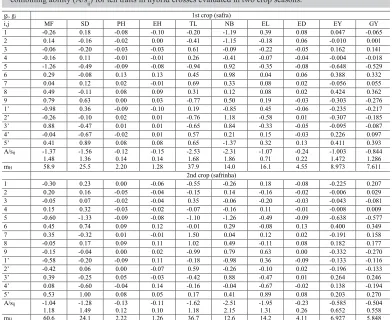
The estimates of the effects of GCA for both groups of varieties (gi - group I; gj - group II) and the maximum and minimum values for the estimates of SCA (sij) within the group of 45 variety crosses are shown in Table 11. High estimates for GCA, either positive or negative, indicate more or less expression of the trait on the average of all crosses involving the respective parent; these effects are then related to the predominantly additive gene action (Sprague and Tatum, 1942). On the other hand, the sij effect expresses the non-additive gene action and is a component of the observed mean in a hybrid combination.
For abbreviations, see Tables 1 or 2. A/sij = range for estimates of specific combining ability effects.
Table 11. Estimates of the mean (mH), effects of general combining ability (gi, gj), and range for specific
combining ability (A/sij) for ten traits in hybrid crosses evaluated in two crop seasons.
gi, gj 1st crop (safra)
i,j MF SD PH EH TL NB EL ED EY GY
1 -0.26 0.18 -0.08 -0.10 -0.20 -1.19 0.39 0.08 0.047 -0.065
2 0.14 -0.16 -0.02 0.00 -0.41 -1.15 -0.18 0.06 -0.010 0.001
3 -0.06 -0.20 -0.03 -0.03 0.61 -0.09 -0.22 -0.05 0.162 0.141
4 -0.16 0.11 -0.01 -0.01 0.26 -0.41 -0.07 -0.04 -0.004 -0.018
5 -1.26 -0.49 -0.09 -0.08 -0.94 0.92 -0.35 -0.08 -0.648 -0.529
6 0.29 -0.08 0.13 0.13 0.45 0.98 0.04 0.06 0.388 0.332
7 0.04 0.12 0.02 -0.01 0.69 0.33 0.08 0.02 -0.056 0.055
8 0.49 -0.11 0.08 0.09 0.31 0.12 0.08 0.02 0.424 0.362
9 0.79 0.63 0.00 0.03 -0.77 0.50 0.19 -0.03 -0.303 -0.276
1’ -0.98 0.36 -0.09 -0.10 0.19 -0.85 0.45 -0.06 -0.235 -0.217
2’ -0.26 -0.10 0.02 0.01 -0.76 1.18 -0.58 0.01 -0.307 -0.185
3’ 0.88 -0.47 0.01 0.01 -0.65 0.84 -0.33 -0.05 -0.095 -0.087
4’ -0.04 -0.67 -0.02 0.01 0.57 0.21 0.15 -0.03 0.226 0.097
5’ 0.41 0.89 0.08 0.08 0.65 -1.37 0.32 0.13 0.411 0.393
A/sij -1.37
1.48 -1.56 1.36 -0.12 0.14 -0.15 0.14 -2.53 1.68 -2.31 1.86 -1.07 0.71 -0.24 0.22 -1.003 1.472 -0.844 1.286
mH 58.9 25.5 2.20 1.28 37.9 14.0 16.1 4.55 8.973 7.611
2nd crop (safrinha)
1 -0.30 0.23 0.00 -0.06 -0.55 -0.26 0.18 -0.08 -0.225 0.207
2 0.20 0.16 -0.05 -0.04 -0.15 0.14 -0.16 -0.02 -0.006 0.029
3 -0.05 0.07 -0.02 -0.04 0.35 -0.06 -0.20 -0.03 -0.043 -0.081
4 0.15 0.32 -0.03 -0.02 -0.07 -0.16 0.11 -0.01 -0.008 0.009
5 -0.60 -1.33 -0.09 -0.08 -1.10 -1.26 -0.49 -0.09 -0.638 -0.577
6 0.45 0.74 0.09 0.12 -0.01 0.29 -0.08 0.13 0.400 0.349
7 0.35 -0.32 0.01 -0.01 1.50 0.04 0.12 0.02 -0.191 0.158
8 -0.05 0.17 0.09 0.11 1.02 0.49 -0.11 0.08 0.182 0.177
9 -0.15 -0.04 0.00 0.02 -0.99 0.79 0.63 0.00 -0.332 -0.270
1’ -0.58 -0.20 -0.09 0.11 -0.18 -0.98 0.36 -0.09 -0.133 -0.116
2’ -0.42 0.06 0.00 -0.07 0.59 -0.26 -0.10 0.02 -0.196 -0.133
3’ 0.39 -0.25 0.05 -0.03 -0.42 0.88 -0.47 0.01 0.264 0.246
4’ 0.08 -0.60 -0.04 0.14 -0.16 -0.04 -0.67 -0.02 0.138 -0.194
5’ 0.53 1.00 0.08 0.05 0.17 0.41 0.89 0.08 0.203 0.270
A/sij -1.04
1.18 -1.28 1.49 -0.13 0.12 -0.11 0.10 -1.62 1.18 -2.51 2.15 -1.95 1.31 -0.23 0.26 -0.585 0.652 -0.504 0.558
mH 60.6 24.1 2.22 1.26 36.7 12.6 14.2 4.11 6.927 5.848
The significance of GCA for the traits directly associates with yield (EY and GY) assures a good perspective for the selection process herein proposed, and before looking to this topic it is readily seen the outstanding parent varieties as indicated by their high and positive effects of GCA; in fact, for GY the higher estimates of gi and gj were shown by NAP-8 in Group I and by HG-5 Group II in the 1st crop; in the 2nd crop the higher estimates were for NAP-6 and HG-5, respectively.
Prediction of population means
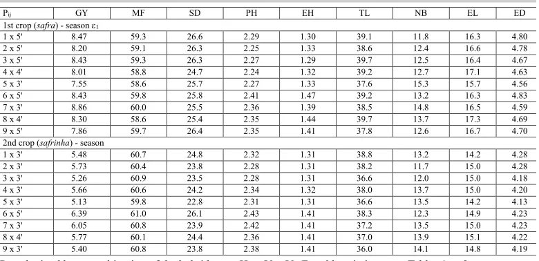
the interpopulation level. By using the procedure already presented, the predicted means of populations identified in (a) are shown in Table 12, for the highest yielding combinations; the predicted means were obtained by first identifying the varieties with positive effects of GCA for grain yield and the prediction procedure was accomplished based only in the selected varieties. Then, the predicted means (Table 12) represent the best combination for each variety of Group I.
Pij - obtained by recombination of the hybrid cross Hij = Vi x Vj. For abbreviations, see Tables 1 or 2.
Table 12. Expected grain yield (t/ha) and eight plant and ear traits of the five highest yielding composites (Pij
for each i) from two groups of populations in two crop seasons.
Pij GY MF SD PH EH TL NB EL ED
1st crop (safra) - season 1
1 x 5' 8.47 59.3 26.6 2.29 1.30 39.1 11.8 16.3 4.80
2 x 5' 8.20 59.1 26.3 2.25 1.33 38.6 12.4 16.6 4.78
3 x 5' 8.43 59.3 26.3 2.27 1.29 39.7 12.5 16.4 4.67
4 x 4' 8.01 58.8 24.7 2.24 1.32 39.2 12.7 17.1 4.63
5 x 3' 7.55 58.6 25.7 2.27 1.33 37.6 15.3 15.7 4.56
6 x 5' 8.43 59.8 25.8 2.41 1.47 39.2 13.2 16.3 4.83
7 x 3' 8.86 60.0 25.5 2.36 1.39 38.5 14.8 16.5 4.59
8 x 4' 8.30 58.6 25.4 2.35 1.44 39.7 13.7 17.3 4.69
9 x 5' 7.86 59.7 26.4 2.35 1.41 37.8 12.6 16.7 4.70
2nd crop (safrinha) - season
1 x 3' 5.48 60.7 24.8 2.32 1.31 38.8 13.2 14.2 4.28
2 x 3' 5.73 60.4 23.8 2.28 1.31 38.2 11.7 15.0 4.28
3 x 3' 5.26 60.9 23.5 2.28 1.31 36.6 12.0 15.0 4.18
4 x 3' 5.66 60.6 24.2 2.34 1.32 38.0 13.7 15.0 4.20
5 x 3' 5.13 59.8 22.8 2.31 1.31 36.6 13.5 14.2 4.13
6 x 5' 6.39 61.0 26.1 2.43 1.41 38.3 12.3 14.9 4.23
7 x 3' 6.05 60.8 23.9 2.42 1.41 37.2 13.5 15.0 4.23
8 x 4' 5.77 60.1 24.4 2.36 1.41 37.0 13.9 15.1 4.22
9 x 3' 5.40 60.8 23.8 2.38 1.41 36.0 14.1 14.8 4.19
In season e1, the expected mean (t/ha) of the selected combinations varied from 7.550 (5 x 3' = NAP-HT x HG-55) to 8.860 (7 x 3' = NAP-PZ x HG-55); the range is equivalent to 95.4 and 106.9% of the check mean. In the 2nd crop (season e2) grain yield varied from 5.130 (5 x 3') to 6.390 (2 x 3' = NAP-FL x HG-55), which represents 97.6 and 108.8% of the check mean. Notice that HG-55 was elected, in both seasons, as the most promising parent variety of Group II to be used as the base for incorporation of two varieties of Group I. In fact, HG-55 ranked in first and second place for positive GCA in the seasons e1 and e2, respectively. The expected means for the other traits of the selected crosses are also shown in Table 12 in order to complement the amount of useful information about the germplasm in use.
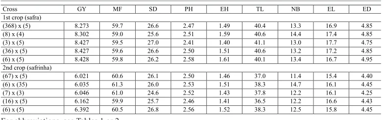
varieties (4, 5). For the season e2, it comprises two varieties (6, 7) and two composites (16 and 67) from Group I, while from Group II it includes two varieties (3, 5) and one composite (35). The next step is to accomplish the crosses following the schedule shown in Table 13.
For abbreviations, see Tables 1 or 2.
Table 13. Expected grain yield and eight plant and ear traits of the five highest yielding crosses between
composites from two groups of populations in two crop seasons.
Cross GY MF SD PH EH TL NB EL ED
1st crop (safra)
(368) x (5) 8.273 59.7 26.6 2.47 1.49 40.4 13.3 16.9 4.85
(8) x (4) 8.302 59.0 25.6 2.51 1.59 40.6 14.4 17.4 4.85
(3) x (5) 8.427 59.5 27.0 2.41 1.40 41.1 13.0 17.7 4.75
(36) x (5) 8.427 59.6 26.6 2.50 1.51 40.6 13.2 17.2 4.85
(6) x (5) 8.428 59.8 26.2 2.58 1.61 40.1 13.4 16.7 4.95
2nd crop (safrinha)
(67) x (5) 6.021 60.6 26.1 2.50 1.46 37.0 11.4 15.4 4.40
(6) x (35) 6.035 61.3 26.0 2.53 1.51 38.3 14.7 16.1 4.45
(7) x (3) 6.046 61.0 24.6 2.52 1.43 37.8 12.2 16.1 4.25
(16) x (5) 6.162 59.9 25.7 2.46 1.41 36.5 12.2 16.6 4.43
(6) x (5) 6.392 60.5 26.8 2.56 1.52 38.3 12.5 15.8 4.45
ACKNOWLEDGMENTS
Research supported by Fundação de Apoio à Pesquisa do Estado de Goiás (FAPEG).
REFERENCES
Andrade JAC and Miranda Filho JB (2008). Quantitative variation in the tropical maize population, ESALQ-PB1. Sci.
Agric. 65: 174-182. http://dx.doi.org/10.1590/S0103-90162008000200011
Basso CW and Miranda Filho JB (2001). Médias preditas de produção de compostos de milho sob severa epidemia de enfezamento no sudeste do Brasil. Summa Phytopathol. 27: 23-30.
CONAB (Companhia Nacional de Abastecimento) (2015). Acompanhamento de safra brasileira: grãos, quarto levantamento, maio 2015 - Brasília: Conab.
Eberhart SA, Harrison MN and Ogada FA (1967). A comprehensives breeding system. Der Zuchter 37: 169-174. Gardner CO and Eberhart SA (1966). Analysis and interpretation of the variety cross diallel and related populations.
Biometric. 22: 439-452. http://dx.doi.org/10.2307/2528181
Geraldi IO and Miranda Filho JB (1988). Adapted models for the analysis of combining ability of varieties in partial diallel crosses. Braz. J. Genet. 11: 419-430.
Goodman MM (1985). Exotic maize germplasm: status and prospects. Iowa State J. Res. 59: 497-527.
Griffing B (1956). Concept of general and specific combining ability in relation to diallel crossing systems. Aust. J. Biol. Sci. 9: 463-493. http://dx.doi.org/10.1071/BI9560463
Hallauer AR and Miranda Filho JB (1988). Quantitative genetics in maize breeding. Iowa State University Press, Ames, 468. Jenkins MT (1934). Methods of estimating the performance of double crosses in corn. J. Am. Soc. Agron. 26: 199-204.
http://dx.doi.org/10.2134/agronj1934.00021962002600030004x
Jenkins MT (1978). Maize breeding during the development and early years of hybrid maize. In: Maize Breeding and
Genetics (Walden DB, ed.) John Wiley, New York, 13-28.
Mather K and Jinks JL (1982). Biometrical Genetics. Chapman and Hall, London.
Mendes UC, Miranda Filho JB, Oliveira AS and Reis EF (2015). Heterosis and combining ability in crosses between two groups of open-pollinated maize populations. Crop Breed. Appl. Biotechnol. 15: 235-243. http://dx.doi. org/10.1590/1984-70332015v15n4a40
Miranda Filho JB and Chaves LJ (1991). Procedures for selecting composites based on prediction methods. Theor. Appl.
Genet. 81: 265-271. http://dx.doi.org/10.1007/BF00215732
Miranda Filho JB and Geraldi IO (1984). An adapted model for the analysis of partial diallel crosses. Braz. J. Genet. 7: 677-688.
Miranda Filho JB and Viégas GP (1987). Milho híbrido. In: Paterniani E and Viégas GP. Melhoramento e produção de milho. Volume I. Campinas: Fundação Cargill, p. 277-340.
Miranda Filho JB, Nass LL, Santos MX and Regitano Neto A (2000). Avaliação de acessos de milho para resistência a doenças foliares. Embrapa Recursos Genéticos e Biotecnologia, Brasília, 147p. (Circular Técnica, 3).
Moro JR, Naspolini Filho V, Viana RT and Gama EEG (1981). Introdução de novos germoplasmas de milho no Brasil.
Pesqui. Agropecu. Bras. 16: 867-882.
Nass LL, Miranda Filho JB and Santos MX (2001). Uso de Germoplasma Exótico no Melhoramento. In: Recursos Genéticos e Melhoramento - Plantas (Nass LL, Valois ACC, Melo IS and Valadares-Inglis MC, eds.). Fundação MT, Rondonópolis, 101-122.
Oliveira AS, Miranda Filho JB and Reis EF (2015). Variability and inbreeding in semiexotic maize populations. Genet.
Mol. Res. 14: 1184-1199. http://dx.doi.org/10.4238/2015.February.6.21
Regitano Neto A, Nass LL and Miranda Filho JB (1997). Potential of twenty exotic germplasms to improve Brazilian maize architecture. Braz. J. Genet. 20: 691-696.
Santos MX and Miranda Filho JB (1992). Genetic potential of two Brazilian races of maize for breeding purposes. J.
Genet. Breed. 46: 83-90.
Souza AC (2015). Variabilidade genética em três populações de milho. Dissertação (Mestrado em Agronomia - Produção Vegetal) - Universidade Federal de Goiás, Regional Jataí, Jataí.
Sprague GF and Tatum LA (1942). General vs. specific combining ability in single crosses of corn. J. Am. Soc. Agron. 34: 923-932. http://dx.doi.org/10.2134/agronj1942.00021962003400100008x