Abstract—Without any infrastructure MANETs need to utilize the broadcast or multicast modes to transfer efficiently packets between wireless nodes. However, broadcast may easily cause a broadcast storm in the wireless networks, which will lead to network congestion and make the normal packets cannot be transferred. This paper tries to combine the advantages of location-aware distributed cluster algorithm and MAOVD schemes to improve the transmission efficiency and the throughput of MANET in geographic routing protocols. We also identify the problems in broadcast storm and bandwidth wasting problems that could be improved by using the design of our LDCA routing protocol for wireless ad-hoc networks.
—Mobile ad-hoc networks, MANET, MAODV, multicast.
I. INTRODUCTION
In recent years, with the upgrading of the wireless infrastructure, more and more mobile Internet users began to notice that the traditional cellular networks need fixed infrastructure-based stations which cost great amounts of time and money. In addition, the signals of wireless network are also susceptible by buildings and topography that makes the network signals become intermittent. On the other hand, mobile ad hoc networks (MANET) does not need traditional infrastructure base station and consider whether the mobile nodes are in the radius range of the base station. Each node can move anywhere and anytime. Nodes communicate with each other like relay transform packets between source node and the destination node. There are many benefits of this communication method, such as when the network infrastructure is incomplete (ex. In the wild mountains, frontline of Warfield, etc.), when the network infrastructure has been destroyed (such as natural disasters, etc.), or in the situation that needs using a wireless network in a short time (ex. speech or exhibition situation) and other cases. Mobile ad hoc networks can connect nodes and transmit messages immediately, so that it can save a lot of construction time and financial costs[1].As shown in Table 1, general cellular network requires a fixed base station; under this circumstances, the expand of time and cost would be higher than MANET.
Manuscript received August 11, 2012; revised September 21, 2012. This work was supported by the National Science Council of Republic of China under grant NSC 100-2221-E-029 -016.
Tzu-Chiang Chiang and Shih-Wei Lin are with the Department of Information Management, Tunghai University, Taiwan, ROC (e-mail:[email protected] )
Jia-Lin Chang is with the Department of Transportation Technology and Management, Kainan University, Taiwan, ROC.
TABLEI:DIFFERENT BETWEEN CELLULAR NETWORKS AND AD-HOC
WIRELESS NETWORKS
Cellular Networks Ad-hoc Wireless Networks
Single-hop wireless links Multi-hop wireless links Fixed infrastructure-based Infrastructure-less Centralized routing Distributed routing High cost of network
maintenance
Low cost of network maintenance
Expensive to deployment Quick to deployment
Based on routing information update mechanism in MANET, it can be divided into three parts, table-driven, on-demand, and hybrid[1], [2].In the Internet, all the nodes of table-driven routing protocols will maintain the network topology information automatically and broadcasting its routing information to surrounding nodes, the represent routing protocol is Destination-Sequenced Distance-Vector Routing (DSDV).On the contrast, on-demand take DSR and AODV as representatives, the nodes do not maintain and broadcasting the routing information automatically and regularly. Only when it is required, they will look for the location of the destination node. Hybrid is the last one which combines the above two categories, such as Zone Routing Protocol (ZRP), GRID. In addition, some scholars have found out that the movement range of MANET has a significant relation with the topography and location of the connecting range. After the general use of global positioning system, scholars have suggested the related researches of location-aware on mobile device [8][9].In the present study, we take location as basis and combine the conception of cluster[9] so that the cluster-header of the partition can manage the routing of the networks and deliver the packets in MANET with more efficiency.
The most commonly technique that MANET used to transmit was flooding broadcast. This technique will abuse and waste the resources and cause network rebroadcast. In the worst case, it will cause a broadcast storm and occupy the bandwidth which makes other packets cannot deliver in the way that they used to be. According to the past studies, they had pointed out that the traditional wire network protocol will cause a lot of problems in the usage of MANET. Those problems include the broadcast storm that come from the packet collision, and make the traditional network protocol cannot perform well in MANET. Therefore, many studies aim to the modification and re-design of the recent protocol, one of them is the multicast routing protocol. In multicast, many scholars had proposed the routing algorithm, for example, Multicast Ad Hoc On-demand Distance Vector Routing(MAODV), MZRP, ODMRP, DCMP, and Distributed clustering algorithm(DCA), etc., all of them are the refinement of wireless multicast routing protocol. The present study uses the existing DCA and MAODV as the
A Location-Based Distributed Routing Algorithm for
Mobile Ad-Hoc Networks
Tzu-Chiang Chiang, Jia-Lin Chang, and Shih-Wei Lin
basis to reinforce the original routing protocol algorithm, hoping to increase the performance of multicast and broadcast in MANET.
II. RELATED WORKS
Many localization schemes have been proposed in the past few years. Most of them are designed for static sensor networks [21], [22], [23], [24], [25].
The purpose of the algorithm written by C. R. Lin and M. Gerla in 1997[7] was to support multimedia traffic. The wireless network layer must guarantee QoS(band-width and delay) to real time traffic components. This approach was consists of two steps to provide QoS to multimedia: (a) the multi hop network was partitioned into the clusters which makes the bandwidth sharing became accomplished in each cluster; (b) to build up the Virtual Circuits with QoS guarantee. Following, we are going to explain the implementation of the above two steps in the multi cluster architecture.
The implementation of clustering algorithm can be found in partitioning the network into clusters. The tradeoff between spatial reuse of the channel and delay minimization can be the main determinant to the size of optimal cluster. The spatial reuse of the channel was drives toward small sizes whereas the delay minimization dives toward large sizes. Moreover, power consumption and geographical layout were applied as the constraints, and the radio transmission power will affect the cluster size. We assumed that in the cluster algorithm, the power of transmission is constant and consist with the network. The nodes in each cluster can communicate with each other in at most two hops. According to their own id of each node, we can construct the clusters. The following algorithm partitions the multi hop network into some non-overlapping clusters. We make the following operational assumptions underlying the construction of the algorithm in a radio network. These assumptions are consistent with most radio data link protocols [3], [4], [6], [7].
1) Every node has a unique ID and knows the IDs of its 1-hop neighbors. This can be pro-vided by a physical layer for mutual location and identification of radio nodes.
2) A message sent by a node is received correctly within a finite time by all its 1-hop neighbors.
3) Network topology does not change during the algorithm execution.
It’s a new scheme that from the node location information of the global positioning system (GPS) and the radio transmission range of the nodes, we can determine a long-life route. Compare with the schemes that use the shortest path, the proposed scheme provided a more stable route and avoid frequent route reconstructions. Long-life route selection mechanism: Each node knows its own location information from the GPS (latitude (s) and longitude (y)), and its current radio transmission range. With the information, each node estimates how long the route will last until the route break down. Contains the source position information and the current transmission range, a source generates a route discovery packet. While in other source-initiated on-demand routing protocols, this packet is propagated to all neighboring
nodes.
The mechanism repeats until the destination receives the discovery packet.
Following the below process, node B receiving the route discovery packet from node A.
1) The location information and radio transmission range of the previous node A recorded in the route discovery and the location information of the receiving node can be used to calculate the FML (forward movement limit) 2) Secondly, using the location information and radio
transmission range of the receiving node B to calculate the BML (backward movement limit)
3) NML (normalized movement limit) = (FML BML)/(FML + BML).
4) Compare NML with the NML stored in the route Discovery packet. Choose the minimum value as the propagated NML stored in the route discovery packet. 5) Forward the route discovery packet to the neighboring
nodes.
III. LOCATION-BASED DISTRIBUTED CLUSTERING ALGORITHM
The present study uses location distributed and multicast cluster algorithm as the base to establish Location-based Distributed clustering algorithm (LDCA). We use LDCA to distribute different amounts of partition which measured of area in a rectangle area and search for the cluster-header in each partition. In the end, we use the way of MAODV to search, establish, and maintain the route.
A. Location-Based Distributed Clustering Algorithm
(LDCA)
First, we set a rectangle area with all nodes in the range and all the nodes know their own coordinates. The start coordinate of the rectangle is (0,0) and the end is (x,y). So the central point of this rectangle area is (x/2,y/2).
Secondly, we distributed the rectangle into several partitions, each partition is 100m*100m and it has their own id. We are trying to find out the node which has the shortest distance from the central point in the each partition. The node then will be set as the cluster-header.
D:the set of ID’s distance to the Center of a Circle
N1:Group_Leader {
Set the AreaStart(0,0); //starting-coordinate Set the AreaEnd(x,y); //end-coordinate Set the Center of a Circle(x/2,y/2); //center
Set my_id (id, (xi,yi),partition_id); //node information
Set the length of the side = L //partition length Partition_id = (xi\L)+(yi\L)(x\L);
//compute the location of node’s partition For(;;) //loop
{
For i = 0 to (x\100)*(y\100)-1; //compute numbers of all partition
Set my_id = cluster_header;
//if the distance to the center point of a node is the minimum; it is the cluster-header
}
If (my_id == Φ) stop; //stop if there does not have any node join
}
B. LDCA Algorithm in Practice
First, we marked the left-top corner as the starting point, the coordinate is marked (0,0). The right-bottom corner is the ending point, marked as (x,y), therefore we can know the central point of the partition is (0+x/2,0+y/2). In this case, we define the length of the side in each partition is 100 meters, so we will get a (x/100*y/100) distributed sub-partition. Each node in the sub-partition will use the GPS to compute and get its own coordinate. We used (xi/100)+(yi/100)(x/100) to
compute the belonging sub-partition of each node. The (xi,yi)
is the coordinate of the node and x is the length of the x axle in the partition.
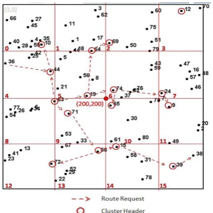
Fig. 1 is a 400 square meter partition which divided with 100 meters. This partition will distributed into 16 sub-partitions, each sub-partition represent a cluster. All the nodes in the cluster will have their own coordinate location; nodes can know their partition through their coordinate. For example, if the coordinate of the node is (132, 257), the coordinate will be located at 1+2*4=9, which is the 9th partition.
Fig. 1. Using LDCA selected the cluster-header in each partition and routing operations.
C. Establish Cluster-Header
Secondly, we will compare the distance between each node and the central point. We will measure the distance between two nodes first and then broadcast out the distance with the central point to other nodes around itself. While other nodes receive the packets, they will compare the partition location of the two nodes. If the nodes were not in the same partition, the packet will be abandoned; on the other hand, if they were in the same partition, the nodes will
compare which one was closer to the central point and find out the closest node to the center point through the above procedure. The closest node then will be the cluster-header in the sub-partition, it will announce message to other nodes in that partition. After other nodes receive the message, they will join the group.
As shown in Fig. 1,node 25 in partition 4 will deliver its message (id, (x,y), partition_id ) to other node, after other neighboring node 42, 44, 36, 28, 55, 10, 4, 35, and 40 received, they will see whether their partition_id is coordinate with node 25. Node 42, 44, and 36 are in the same partition as node 25, so they will keep this packet, other nodes which are not in the same partition will abandon this packet. After that, node 42, 44, and 36 will compare with node 25 the distance to the central point (200,200). Node 44 will inform other nodes that it has the closest distance to the central point. Eventually, node 44 will repeat this procedure until the cluster-header in that partition is selected. The other nodes in that partition will join in and become a group.
D. Path establish and Packet Delivery
After the cluster-header was selected in each partition, if transmit packet to the node in other partition was need, the node have to transmit the packet to the cluster-header in its partition. As the cluster-header received the source node packets, it will transmit to the destination node. Before the route was established, we will search the destination node through the following procedure.
1) When the source node needs to deliver packet to the destination node, it will broadcast the packet of RREQ to its cluster-header, the cluster-header will broadcast out to look for the destination node.
2) After RREQ reach the destination node, the destination node will deliver RREP packet to reply the source node. 3) Both RREQ and RREP packets will be delivered by the
cluster-header.
4) Each cluster-header on the routing table will note down the transmitting routing information.
5) The information gathered by RREQ and RREP and other routing information will be preserved in routing table. When the source node wants to transmit a packet to a certain destination node, it will ask its cluster-header whether there is a routing information first. The cluster-header will check its routing table to determine whether there is a route to reach the destination node exists. If the path is existed, it will relay transmit the packet from next cluster-header to the destination node. If there is no path in the routing table, the source node has to broadcast RREQ packet to the nearby cluster-header. The RREQ packet includes source IP address, destination node IP address, and the unique id of the node.
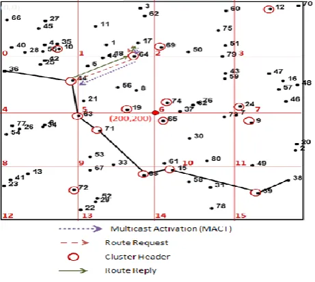
transmitted to the cluster-header node 39 in partition 15. In Fig. 2, after the location of node 38 was confirmed, node 38 will reply RREP to node 44 in partition 4, and transmit MACT from node 36 to the cluster-header 38. From this time on, the cluster tree was established. Node 36 can transmit packets to node 38 through the cluster-header. In Fig. 2, the multicast tree was established.
Fig. 2. A multicast tree.
IV. SIMULATION RESLUTS
The present study simulated an experiment to discuss whether the size of the region partition and the number of cluster-header will affect the performance of Internet transition in region partition. We separated the partition size into un-partition, 2*2 partition and 4*4 partition types. Also, the protocol of wireless network was using MAODV, the area was 800m*800m and the transition range of wireless nodes was 150m, whereas the numbers of nodes were 50. In addition, the present study used network simulator-NS2 to simulate the packet delay, packet jitter and the throughput in different partition size during packets transition.
Fig. 3 is the result of packet delay. At first, under the unpartition situation, the more partition , the longer delay time of the packets. However, after the cluster header was confirmed, the transfer of the nodes become faster, the packet delay will gradually become lower and the packet delay area of the unpartion area will become higher instead
Fig. 3. The comparisons of the packet delay in different partitions.
The above Fig. 4 is the packet jitter. The packet jitter was lower than the other two situations in the 4*4 location distributed. But under the un-partition and the 2*2 partition situation, which the partition is too small, there is no siginificant difference in the Fig. 17.
Fig. 4. The comparisons of the packet jitter in different partition.
The Fig. 5, Fig. 6, and Fig. 7, and 8 below are the average comparisons of delay time. When there are few nodes, such as 30 and 40 nodes, the sparse node will lead lower delay time; in this case, the delay time will go for a smooth trend. At this time the number of partition will not cause much difference.
Fig. 5. The comparisons of the delay time in different partition at 30 nodes.
Fig . 6. The comparisons of the delay time in different partition at 40 nodes.
Fig. 7. The comparisons of the delay time in different partition at 50 nodes.
Fig. 8. The comparisons of the delay time in different partition at 60 nodes
V. DISCUSSION AND CONCLUSION
into the destination speedily. However, node broadcast can easily cause broadcast storm in the networks, which will lead to network congestion and make the normal packet cannot be transferred. The present study tries to combine the advantages of distributed cluster algorithm, location-aware and MAOVD. With the hope of improve the transmission range and the rate of MANET in geographic routing protocols.
According to the experiment data, the partition situation is more efficient than un-partition, especially under the 4*4 and 2*2 situations. However, high-density partition will cause a complicate routing which is worse than the un-partition location. Take our experiment for example; the more close the transmission distance between nodes to the diagonal distance of the partition rectangle area, the result of the experiment will be better. For that it represent the cluster header can handle the normal nodes in the whole partition. Our future work will take the transmission range and the change of mobile path in each node as the objectives of next experiment, includes optimize the efficiency, mobility and comprehensive performance of end-to-end. Furthermore, we can extend the experiment on the irregular location instead of the rectangle location.
ACKNOWLEDGMENT
This work was supported by the National Science Council of Republic of China under grant NSC 100-2221-E-029 -016.
REFERENCES
[1] E. M. Royer and C. K. Toh, “A review of current routing protocols for ad hoc mobile wireless networks,” IEEE Personal Communications, vol. 6, no. 2, pp. 46-55, 1999.
[2] A. A. Papadopoulos and J. A. McCann, “Towards the design of an energy-efficient, location-aware routing protocol for mobile, ad-hoc sensor networks,” Proceedings of the Database and Expert Systems Applications, 15th International Workshop on (DEXA'04), pp. 705-709, 2004.
[3] C. Y. Chang and C. T. Chang, “Hierarchical cellular-based management for mobile hosts in Ad-hoc wireless networks,” Computer Communications, vol. 24, no.15-16, pp. 1554-1567, 2001.
[4] C. E. Perkins, “Ad hoc networking,” Addison-Wesley Professional, 1stedition., 2008.
[5] C. E. Perkins, E. M. Royer, and S. Das, “Ad hoc on-demand distance vector (AODV) routing,” IETF RFC 3561, 2003.
[6] D. Johnson, “The dynamic source routing protocol for mobile Ad Hoc networks (DSR),” RFC 4728, 2003.
[7] C. R. Lin and M. Gerla. “Adaptive clustering for mobile wireless networks,” IEEE Journal on Selected Areas in Communications, vol. 15, no. 7, pp. 1265-1275, 1997.
[8] F. A. Khan and W. C. Song, “A location-aware zone-based routing protocol for mobile Ad hoc networks,” The Joint International Conference on Optical Internet and Next Generation Network, COIN-NGNCON, 2006.
[9] C. T. Cheng, C. K. Tse, and C. M. Lau, “A bio-inspired coverage-aware scheduling scheme for wireless sensor networks,” Vehicular Technology Conference, pp. 223-227, 2008.
[10] H. Wang, X. Zhang, and A. Khokhar, “Efficient void handling in contention-based geographic routing for wireless sensor networks,” IEEE Global Telecommunications Conference, pp. 663-667, 2007. [11] X. Xiang, X. Wang, and Y. Yang, “Stateless multicasting in mobile Ad
hoc networks,” IEEE Transactions on Computers, vol. 59, no. 8, 2010. [12] S. Rohini and K. Indumathi, “Consistent cluster maintenance using probability based adaptive invoked weighted clustering algorithm in MANETs,” National Conference on Innovations in Emerging Technology, pp. 37-42, 2011.
[13] J. P. Shen, W. K. Hu, and J. C. Lin, “Distributed localization scheme for mobile sensor networks,” IEEE Transaction on Mobile Computing, vol. 9, no. 4, pp. 516-526, 2010.
[14] C. Liu and K. Wu, “Performance evaluation of range-free localization methods for wireless sensor networks,” 24th IEEE International Performance, Computing, and Communications Conference, pp. 59-66, 2005.
[15] C. Liu, K. Wu, and T. He, “Sensor localization with ring overlapping based on comparison of received signal strength indicator,” IEEE International Conference on Mobile Ad-Hoc and Sensor Systems, pp. 516-518, 2004.
[16] J. P. Sheu, P. C. Chen, and C. S. Hsu, “A distributed localization scheme for wireless sensor networks with improved grid-scan and vector-based refinement,” IEEE Transactions on Mobile Computing, vol. 7, no. 9, pp. 1110-1123, 2008.
[17] V. Vivekanandan and V. W. S. Wong, “Concentric anchor-beacons (CAB) localization for wireless sensor networks,” IEEE International Conference on Communications, vol. 9, pp. 3972-3977, 2006. [18] C. S. R. Murthy and B. S. Manoj, “Ad hoc wireless networks:
architectures and protocols,” Prentice Hall Professional Technical Reference Upper Saddle River, 2004.