A Method of Computing Functions of Trapezoidal Fuzzy Variable and Its Application to Fuzzy Calculus

A Method of Computing Functions of Trapezoidal Fuzzy Variable and Its

Application to Fuzzy Calculus

Muhammad Zaini Ahmada,*_{, Mohammad Khatim Hasan}b a_{Institute for Engineering Mathematics, Universiti Malaysia Perlis}

02000 Kuala Perlis, Perlis, Malaysia

b_{School of Information Technology, Faculty of Information Science and Technology} Universiti Kebangsaan Malaysia

43600 UKM Bangi, Selangor, Malaysia *Corresponding email: [email protected]

Abstract

This paper introduces a method of computing functions of trapezoidal fuzzy variable. The method is based on the implementation of an unconstrained optimisation technique over the -cut of fuzzy interval. To show the effectiveness of the proposed method, we provide several numerical examples in computing the solutions of linear and non-linear fuzzy differential equations. The final results showed that the proposed method is capable to generate convex fuzzy solutions on time domain.

1. INTRODUCTION

In fuzzy set theory, the extension principle has been extensively used in many areas of discipline, namely in fuzzy optimisation problem (Shiang-Tai, 2004), fuzzy differential equation (Ma et al., 1999), fuzzy dynamical system (Ahmad and De Baets, 2009) and many more. Basically, the extension principle is the theoretical basis of fuzzy arithmetic, i.e., a process of extending real-valued functions to functions accepting fuzzy interval as arguments. The idea is very simple, but in practice, it is a complex problem.

Recently, Ahmad and Hasan (2011) have proposed an efficient computational method in order to compute functions accepting fuzzy interval as arguments. The proposed method is easy to implement and can be used in many practical problems. The convexity of fuzzy output is also guaranteed. In this paper, we will demonstrate the capability of the proposed method in order to approximate the solutions of linear and non-linear fuzzy differential equations.

2. THE EXTENSION PRINCIPLE

The extension principle (Zadeh, 1975a, Zadeh, 1975b) becomes an important tool in fuzzy set theory and applications. The idea is that each function f :UV induces another function

: ( ) ( )

f F U F V defined for each fuzzy set A in U by

        . range(f) y if , 0 , range(f) y if , ) ( sup = ) )(

( 1( )

x A y

A

f x f y (1)

If f is one to one mapping, we have

       . range(f) y if , 0 , range(f) y if , )) ( ( = ) )( ( 1 _y f A y A

f (2)

To demonstrate the extension principle, we consider f R: R defined by 3

2 = ) (x x

f

and the fuzzy interval AR (a fuzzy set defined on real line) is given by

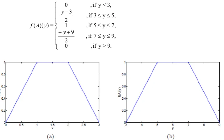
                . 3 > x if , 0 , 3 x 2 if , 3 , 2 x 1 if , 1 , 1 x 0 if , , 0 < x if , 0 = ) ( x x x

A (3)

  

   

 

  

  

  

. 9 > y if , 0

, 9 y 7 if , 2

9

, 7 y 5 if , 1

, 5 y 3 if , 2

3 ,ify<3, 0

= ) )( (

y y y A

f (4)

Figure 1: (a) The trapezoidal fuzzy interval A; (b) The output from the extension principle.

The graphs of (3) and (4) are depicted in Figs. 1(a) and 1(b), respectively. In general, if f is non-monotone function, then the calculation of (1) is not an easy task. This needs a contribution on developing an efficient computational algorithm for computing (1).

3. THE METHOD

Let A=(a,b,c,d) be a trapezoidal fuzzy interval. The -cut of A is denoted by [A] =[a1,a2] for (0,1], where a1 =a(ba) and b2 =d(dc). First, we discretise  in the form

n

n 

 

0 < 1<...< 1< , where 0 =0 and n =1. The discretised  are equally spaced, that is h

j j =0 

 , for j=0,1,2,...,n and =1>0 n h

 . In this study, h is called the discretisation spacing. After discretisation, we have a set of  with (n1) elements:





 (5) This leads to a set of I with (n1) intervals:

   



_{A A} j _A n

I= [ ]0,...,[ ] ,...,[ ] ₍₆₎

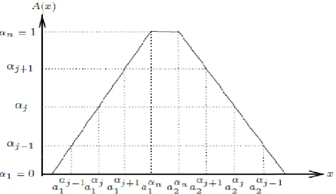
For the different -cuts of A the following property holds (Möler and Reuter, 2007):

. with

[0,1] ,

, ] [ ]

[A j1  A j j j1 jj1

 

Figure 2. -discretisation of a trapezoidal fuzzy interval (Ahmad and Hasan, 2011). Since this property holds for all [0,1], the -cuts of A can be constructed as the union of sub-intervals as shown in the following equation (see Fig. 2):

.] , [ ] , [ ] , [ = ]

[Aj a₁j a₁j1  a₁j1 a₂j1  a₂j1 a₂j (8) Let f R: R be a continuous function. Given a fuzzy interval A defined in R. In order to find

) ( = f A

B at each level of j for j=0,1,2,...,n, we need to solve the following equations:

, ) ( min ), ( min ), ( min min = ] 2 , 1 2 [ ] 1 2 , 1 1 [ ] 1 1 , 1 [ 1                  x f x f x f b j a j a x j a j a x j a j a x j        (9) . ) ( max ), ( max ), ( max max = ] 2 , 1 2 [ ] 1 2 , 1 1 [ ] 1 1 , 1 [ 2                  x f x f x f b j a j a x j a j a x j a j a x j        (10)

Then, by using linear spline interpolation we interpolate the desired results (b₁j,_j) as well as )

, (b₂j j



to obtain a fuzzy interval B. The next section, we will use this method in order to approximate the solution of fuzzy differential equations.

4. NUMERICAL EXAMPLES

In this section, we provide two numerical examples of computing the solution of linear and non-linear fuzzy differential equations. For this purpose, the method proposed in Section 3 will be incorporated into the generalised fuzzy Euler method proposed by Ahmad and Hasan (2010). Example 1 Consider the linear fuzzy differential equation:

      , (1,2,3,4) = (0) , [0,1] , 3 2 = ) ( Y t Y t

According to Ahmad et al. (2011), we need to solve the following system of ordinary differential equations:

   

  

 

. 4 = (0) ,

3 2 = ) (

, 1 = (0) ,

3 2 = ) (

2 2

2

1 1

1

 

 



 



y y

t y

y y

t y

' '

(12)

The analytical solutions of (12) are , 3/2 )

(5/2 = )

( 2

1 t  e t

y 

. 3/2 )

(11/2 = )

( 2

2 t  e t

y  .

It is clear that

)] ( ), ( [ = )] (

[Y t  y1 t y2 t

is the solution of fuzzy differential equation (11). It is illustrated in Fig. 3(a).

Figure 3. (a) The exact solution of Example 1; (b) The approximate solution of Example 1 with 0.02

=

h and N =50.

Using the generalised fuzzy Euler method (Ahmad and Hasan, 2010), the results are shown in Fig. 3(b). From the graph, we can see that the approximate solution converges to the exact solution. The numerical results of exact and approximate solution, and their errors at t=0.5 are listed in Table 1.

Table 1: The numerical results of Example 1 at t=0.5

 _(0.5)

1

y y0.5,1 E0.5,left y2(0.5) y0.5,2 E0.5,right

Example 2 Consider the non-linear fuzzy differential equation:

  

 _

. ) /4, /2,3 (0.2, = (0)

, [0,4] ,

) ( sin = ) (

  

Y

t tY t

Y'

(13)

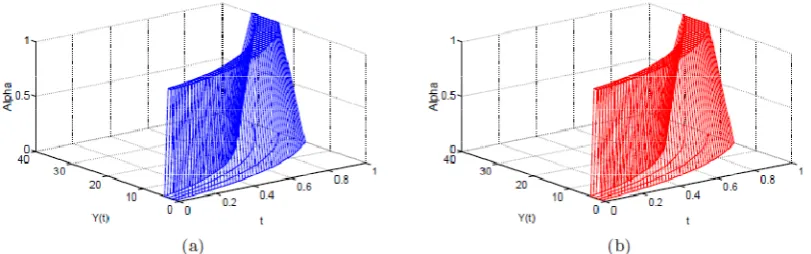
Since the exact solution of (13) cannot be found analytically, we approximate its solution using the generalised fuzzy Euler method (Ahmad and Hasan, 2010). Using the step size h=0.04 and

100 =

N , we obtain the approximate solution of (13) as plotted in Fig. 4(a). From the graph, we can see that the approximate solution of (13) is periodic as t increases. However, if we use the conventional fuzzy Euler method (Ma et al., 1999), the approximate solution of (13) is diverging as t increases (see Fig. 4(b)). This shows us that the generalised fuzzy Euler method is capable to generate periodic solution on the time domain.

Figure 4: (a) The approximate solution of Example 2 using the method proposed by Ahmad and Hasan (2010); (b) The approximate solution of Example 2 using the method proposed by Ma et

al. (1999).

5. CONCLUSIONS

In this paper, we have introduced a method of computing functions of a trapezoidal fuzzy variable. The method has two advantages: (a) the convexity of the output is ensured even if f is a non-monotone function; (b) it can be incorporated into any numerical method in order to approximate the solution of linear and non-linear fuzzy differential equations. This is a stronger requirement since there is no attention has been made, especially in solving non-linear fuzzy differential equations.

Acknowledgment

This research was co-funded by the Ministry of Higher Education of Malaysia (MOHE) and partially supported by Universiti Malaysia Perlis (UniMAP) under the programme “Skim Latihan Akademik IPTA (SLAI)”.

REFERENCES

Ahmad, M. Z. and De Baets, B. (2009). A Predator Prey Model with Fuzzy Initial Populations. In Proc. of the Joint

13th International Fuzzy Systems Association World Congress and 6th Conference of the European Society for Fuzzy Logic and Technology, pp:1311-1314.

Ahmad, M. Z. and Hasan, M. K. (2010). A New Approach to Incorporate Uncertainty into Euler Method. Applied

Equations. Submitted for publication.

Ahmad, M. Z. and Hasan, M. K. (2011). Incorporating Optimisation Technique into Zadeh's Extension Principle for

Computing Non-Monotone Functions with Fuzzy Variable. To be published.

Ma, M., Friedman, M. and Kandel, A. (1999). Numerical Solution of Fuzzy Differential Equations. Fuzzy Sets and

Systems, 105: 133-138.

Mizukoshi, M. T., Barros, L. C., Chalco-Cano, Y., Román-Flores, H. and Bassanezi, R. C. (2007). Fuzzy Differential

Equations and The Extension Principle. Information Sciences, 177: 3627-3635.

Möler, B. and Reuter, U. (2007). Uncertainty Forecasting in Engineering. Springer-Verlag, Berlin Heidelberg.

Shiang-Tai, C. K. (2004). Solving Fuzzy Transportation Problems Based on Extension Principle. European Journal of

Operational Research, 153: 661-674.

Zadeh, L. A. (1975a). The Concept of A Linguistic variable and Its Application in Approximate Reasoning, I, II. Information Sci., 8: 199-251, 301-357.