Fuzzy MCDM Model for Risk Factor Selection in Construction Projects

(1)

FUZZY MCDM MODEL FOR RISK FACTOR SELECTION IN

CONSTRUCTION PROJECTS

Pejman Rezakhani

Department of Architecture and Civil Engineering, Kyungpook National University, Korea

*Corresponding E-mail : [email protected]

ABSTRACT

Risk factor selection is an important step in a successful risk management plan. There are many risk factors in a construction project and by an effective and systematic risk selection process the most critical risks can be distinguished to have more attention. In this paper through a comprehensive literature survey, most significant risk factors in a construction project are classified in a hierarchical structure. For an effective risk factor selection, a modified rational multi criteria decision making model (MCDM) is developed. This model is a consensus rule based model and has the optimization property of rational models. By applying fuzzy logic to this model, uncertainty factors in group decision making such as experts` influence weights, their preference and judgment for risk selection criteria will be assessed. Also an intelligent checking process to check the logical consistency of experts` preferences will be implemented during the decision making process. The solution inferred from this method is in the highest degree of acceptance of group members. Also consistency of individual preferences is checked by some inference rules. This is an efficient and effective approach to prioritize and select risks based on decisions made by group of experts in construction projects. The applicability of presented method is assessed through a case study.

Keywords: Multi criteria decision making; Risk management; Fuzzy set; Construction management

1.0 INTRODUCTION

(2)

International Journal of Sustainable Construction Engineering & Technology (ISSN: 2180-3242) Vol 3, Issue 2, 2012

2.0 RISK

CLASSIFICATION

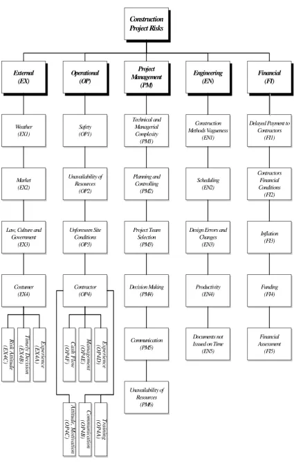
PMBok Version 2008 [1] defines risk classification as a provider of a structure that ensures a comprehensive process of systematically identifying risks to a consistent level of detail and contributes to the effectiveness and quality of the identify risks process. Risk classification is an important step in the risk assessment process, as it attempts to structure the diverse risks that may affect a project. There are many approaches in literature for construction risk classification. Perry and Hayes [2] give an extensive list of factors assembled from several sources, and classified in terms of risks retainable by contractors, consultants and clients. Abdou [3] classified construction risks into three groups, i.e. construction finance, construction time and construction design. Shen [4] identified eight major risks accounting for project delay and ranked them based on a questionnaire survey with industry practitioners. Tah and Carr [5] classified project risks by using the hierarchical risk breakdown structure (HRBS) and classified them into internal and external risks. Chapman [6] grouped risks into four subsets: environment, industry, client and project. Shen [7] categorized them into six groups in accordance with the nature of the risks, i.e. financial, legal, management, market, policy and political. Chen et.al. [8] proposed 15 risks concern with project cost and divided them into three groups: resource factors, management factors and parent factors. Assaf and Al-Hejji [9] mentioned the risk factors as the delay factors in construction projects. Dikmen et al [10] used influence diagrams to define the factors which have influence on project risks. Zeng et al. [11] classified risk factors as human, site, material and equipment factors. Based on the above literature review, we propose risk classification as shown in figure 1.

3.0 RISK FACTOR PRIORITIZATION AND SELECTION

After classifying the inherent risks in construction projects, it is very important to select and prioritize the risk items in order to have an efficient risk management plan. Since we have a finite number of criteria and infinite number of feasible alternatives, the multiple criteria decision making model should be utilized. The main factors that taken into consideration in mentioned model are decision makers influence weights, their preferences for risk factor selection and the criteria for assessing risks. Group members consist of different experts in construction industry with variety in experience, knowledge and expertise. Experts with higher degree of competence should be assigned higher weights. Experts may not know or consider all the relevant information for a decision problem. To conquer this subject, an uncertainty factor named preference of every decision maker and related belief matrices are considered.

(3)

Figure 1: Construction Risk Classification Construction Project Risks Project Management (PM) Engineering (EN) Operational (OP) External (EX) Financial (FI)

Delayed Payment to Contractors (FI1) Contractors Financial Conditions (FI2) Inflation (FI3) Funding (FI4) Financial Assessment (FI5) Construction Methods Vagueness (EN1) Technical and Managerial Complexity (PM1) Scheduling (EN2)

Design Errors and Changes

(EN3)

Productivity (EN4)

Documents not Issued on Time

(EN5) Planning and Controlling (PM2) Project Team Selection (PM3) Unavailability of Resources (OP2) Communication (PM5) Safety (OP1) Contractor (OP4) Decision Making (PM4) Unforeseen Site Conditions (OP3) Weather (EX1) Market (EX2)

(4)

3.1 METHODOLOGY

Let P{ , ,..., },P P1 2 Pn n2 be a given number of experts in the decision making group to prioritize and select risks from classified risk factors. The proposed model has ten steps within three stages:

Stage 1: Risk factor, assessment criteria and experts` influence weights determination

Step 1: By proposing classified risks in a group, every expert may have one or several

possible risk factor selection. Through discussions and summarizations, S { , ,...,S S₁ ₂ S_m},m2

is selected from alternative pool as final risk factors (alternatives) for prioritization.

Step 2: A criterion pool is constructed in this step and every members` assessment criteria is put into this pool. Each expert can propose his own assessment criteria for ranking and

assessing the risk factors in this pool. Top T criteria, C { ,C C₁ ₂,..., }C_t are chosen as assessment

criteria for risk selection problem.

Step 3: To consider the experience, knowledge and expertise of each expert, an influence weight is described and assigned to every expert. These influence weights are described by

linguistic term v_k,k 1,2,...,n.These weights can be determined through discussions in group or

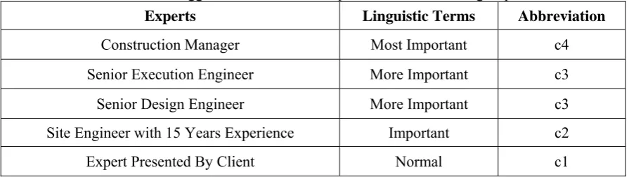
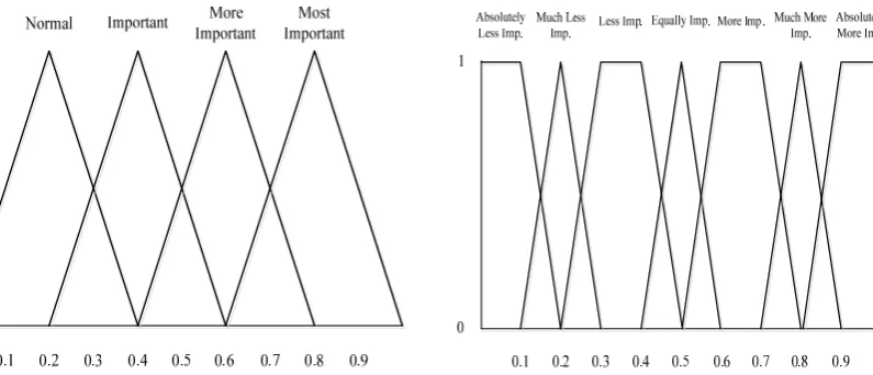
assigned by the leader of decision making group. These weights are assigned before or at the beginning of decision process. Table 1 shows related linguistic terms of decision makers. These linguistic terms and related membership functions are shown in figure 2. Triangular fuzzy numbers are used to map the linguistic terms to their corresponding fuzzy numbers. Table 2 presents a suggestive construction expert board to deal with risk selection in construction projects.

Table 1: Linguistic terms for describing weights of decision makers Linguistic

Terms

Membership Functions

Fuzzy Numbers

Supporting

Intervals Abbreviation

Normal 5x (0,0.2,0.4) 0 ≤ x ≤ 0.2 c1

2-5x 0.2 ≤ x ≤ 0.4

Important 5x-1 (0.2,0.4,0.6) 0.2 ≤ x ≤ 0.4 c2

3-5x 0.4 ≤ x ≤ 0.6

More Important 5x-2 (0.4,0.6,0.8) 0.4 ≤ x ≤ 0.6 c3

4-5x 0.6 ≤ x ≤ 0.8

Most Important 5x-3 (0.6,0.8,1) 0.6 ≤ x ≤ 0.8 c4

5-5x 0.8 ≤ x ≤ 1

Table 2: Suggestive construction expert board in decision group

Experts Linguistic Terms Abbreviation

Construction Manager Most Important c4

Senior Execution Engineer More Important c3

Senior Design Engineer More Important c3

Site Engineer with 15 Years Experience Important c2

(5)

Figure 2: M.F. of decision makers weights Figure 3: M.F. of assessment criteria comparison

Stage 2: Expert preference generation

Step 4: In this step each expert by using a pair-wise comparison expresses his opinion

about outcomes of step 2. At first, a pair-wise comparison matrix k

ij t t

E e



 

   is established. Every member of this matrix represents the quantified judgments on pairs of assessment criteria

( , 1, 2,..., , )

i j

C and C i j  t i  j . The linguistic terms and corresponding membership values which

will be used for the comparison of the assessment criteria are described in Table 3 and figure 3. By utilizing the political model in this hybrid system, there is no obligation for experts to compare all the outcomes. Where ever the experts do not know or cannot compare the relative importance

of assessment criteria C and C_i _j a ‘*’ sign will be placed in pair-wise comparison matrix. By

using following linguistic inference rules, the inconsistency of each pair-wise comparison matrix k

ij t t

E e



 

   is corrected:

Rule 1: Positive-Transitive rule;

max( , )

( 4,5,6,7) ( 4,5,6,7), .

k k k

ij s jm t im s t

If e a s  and e a t  then e a

Rule 2: Negative-Transitive rule;

min( , )

( 3, 2,1) ( 3, 2,1), .

k k k

ij s jm t im s t

If e a s  and e a t  then e a

Rule 3: De-In-Uncertainty rule;

( 4,5,6,7) ( 3, 2,1) '*', '*'.

k k k

ij s jm t im i

If e a s  and e a t  or then e a for any t  i s or

Rule 4: In-De-Uncertainty rule;

( 3, 2,1) '*', ( 4,5,6,7), '*'.

k k k

ij s jm t im i

If e a s  or and e a t  then e a for any s i t or

After calculating the comparison matrix k

ij t t

E e



 

   by using the geometric mean of each

row, consistent weights k( 1, 2,..., )

i

w i  t for every risk selection criterion is calculated. Resulting

fuzzy numbers are normalized and described as

0

* 1

1,2,..., ; 1,2,..., , ( ).

R

k

k i k

i _t i T

k i i

w

w for i t k n w F R

w



   



(6)

Table 3: Linguistic terms for the comparison of assessment criteria Linguistic Terms Membership

Functions

Supporting

Absolutely Less Important

0

(0,0,0.1,0.2)

x=0

a1

1 0 ≤ x ≤ 0.1

2-10x 0.1 ≤x ≤ 0.2

Much Less Important

10x-1 _{(0.1,0.2,0.2,0.3)} 0.1 ≤ x ≤ 0.2 _a2

3-10x 0.2 ≤ x ≤ 0.3

Less Important

10x-2

(0.2,0.3,0.4,0.5)

0.2 ≤ x ≤ 0.3

a3

1 0.3 ≤ x ≤ 0.4

5-10x 0.4 ≤ x ≤ 0.5

Equally Important 10x-4 (0.4,0.5,0.5,0.6) 0.4 ≤ x ≤ 0.5 a4

6-10x 0.5 ≤ x ≤ 0.6

More Important

10x-5

(0.5,0.6,0.7,0.8)

0.5 ≤ x ≤ 0.6

a5

1 0.6 ≤ x ≤ 0.7

8-10x 0.7 ≤ x ≤ 0.8

Much More Important

10x-7

(0.7,0.8,0.8,0.9) 0.7 ≤ x ≤ 0.8 a6

9-10x 0.8 ≤ x ≤ 0.9

Absolutely More Important

10x-8

(0.8,0.9,1,1)

0.8 ≤ x ≤ 0.9

a7

1 0.9 ≤ x ≤ 1

0 x=1

Step 5: To express the possibility of selecting a risk factor by experts, a belief level is

introduced. The belief level k( 1, 2,..., , 1, 2,..., , 1, 2,..., )

ij

b i  t j  m k  n belongs to a set of linguistic

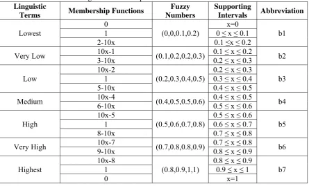
terms that contain various degrees of preferences required by decision makers. Where ever an expert do not know or cannot give a belief level a ‘**’ sign is used in belief matrix. The linguistic terms for preference belief levels of alternatives are described in table 4.

Table 4: Linguistic terms for preference belief levels for alternatives Linguistic

Terms Membership Functions

Supporting

Lowest

0

(0,0,0.1,0.2)

x=0

b1

1 0 ≤ x ≤ 0.1

2-10x 0.1 ≤x ≤ 0.2

Very Low 10x-1 (0.1,0.2,0.2,0.3) 0.1 ≤ x ≤ 0.2 b2

3-10x 0.2 ≤ x ≤ 0.3

Low

10x-2

(0.2,0.3,0.4,0.5)

0.2 ≤ x ≤ 0.3

b3

1 0.3 ≤ x ≤ 0.4

5-10x 0.4 ≤ x ≤ 0.5

Medium 10x-4 (0.4,0.5,0.5,0.6) 0.4 ≤ x ≤ 0.5 b4

6-10x 0.5 ≤ x ≤ 0.6

High

10x-5

(0.5,0.6,0.7,0.8)

0.5 ≤ x ≤ 0.6

b5

1 0.6 ≤ x ≤ 0.7

8-10x 0.7 ≤ x ≤ 0.8

Very High 10x-7 (0.7,0.8,0.8,0.9) 0.7 ≤ x ≤ 0.8 b6

9-10x 0.8 ≤ x ≤ 0.9

Highest

10x-8

(0.8,0.9,1,1)

0.8 ≤ x ≤ 0.9

b7

1 0.9 ≤ x ≤ 1

(7)

Step 6: By applying the normalized weights resulted from step 4 into belief level matrix ( k)( 1, 2,..., )

ij

b k  n and aggregate the results, belief vectors

1 1 2 2 ... s s

k k k k k k k

j j jj j jj j jj

b w b w b  w b

where ( 1, 2,..., ) '**'

i

k jj

b i  s is not are obtained.

Step 7: At this step, normalized weight of decision maker is calculated.

0

*

1

1, 2,..., . k

k n _R

i i v

v for k n

v 

 





Step 8: By applying the normalized weight obtained from previous step and belief vectors obtained from step 6, a weighted normalized fuzzy decision matrix is constructed.

1 1 1

1 2

2 2 1

* * * 1 2 *

1 2 1 2 ₁

1 2

( , ,..., ) ( , ,..., ) .

m

n _k

m

m n j _k k j

n n n

m

b b b

r r r v v v where r v b

b b b

        _ _       



              

Step 9: The ideal solution is assessed and the distance between alternatives (risk factor) and the ideal solution will be calculated. Alternative (risk factor) with the least distance is assumed to be the highest priority risk factor selected by group decision.

Suppose elements in decision matrix defined as ( L, M, R)

m m m m

r  r r r and the ideal alternative is

named * _[ *_{] :} * ₍ *L_, *M_, *R₎

j j j j j

A  x b  x x x . The distance between every alternative in decision matrix

and ideal alternative is calculated as follow:



 



*

2 2 2

* * * ( , ) 1 1 3 m m

L L M M R R

i r A m j m j m j

j

d d r x r x r x

     _      _  





Assume that decision matrix is a set of pairs (rK, )rL that

r

K is preferred to rL. This

implies that risk factor K has more effect on project objectives than risk factor L and distance

( )di between risk factor K to ideal set of alternatives (risk items) is less than risk factor L

(dL dK). As we stated before, experts may have no or incomplete information about assessment

criteria; so we the human errors in prediction should be considered. This error (d) and the

amount of incredibility (error) in pair-wise comparison of alternatives ( )B to find the negative

ideal solution is defined as bellow:

, ₀K L K L

K L

K L

d d d d

d

d d

 _{ }  

 

, max{0, }

K L K L

d  d d

, ( , ) m

K L K L r

B d









To obtain the positive ideal solution, a new value called credibility judgment degree is defined between two risk factors K and L.

, ₀L K L K

K L

L K

d d d d

d

d d

 _{ }  

 

, max{0, }

K L L K

d  d d

, ( , ) m

K L K L r

G d









To obtain the final ideal solution, credibility degree should be maximized while

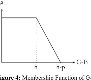
incredibility (error) degree should be minimized. Amount of this difference ( )h and Pshould be

defined by decision makers (G B h). The membership function of this ideal solution is as

(8)

( , )

( )

( ) ( )

( ) ( ) m

L K

K L r G B

d d h P

G B h P

P P

 _ 

  

 





In the field of risk selection in construction projects, h can be the defined as the least

effect of a risk item in project objective and amount of P can be described as the highest effect of

a risk item. The membership function of GB is shown on figure 4.

Figure 4: Membership Function of G-B

The distance ( )di of alternatives (risk factors) with ideal solution (G-B) is calculated.

The risk factor with the least distance is selected as the highest priority factor to be considered and other factors will be ranked in ascending order.

4.0 COMPARING THE PROPOSED FUZZY MCDM MODEL WITH FUZZY

AHP

In this section, a comparison between proposed fuzzy MCDM model and different fuzzy AHP approaches is presented. This part of the paper is followed by definition of AHP, Fuzzy AHP, their shortcomings and benefits of our model comparing to fuzzy AHP.

4.1 AHP

The AHP is a popular decision making technique that has proven easy to understand and plausible for prioritizing alternatives among multi-criteria and multi-attributes (Saaty, 1990, Kim, Whang, 1993, Cheng, 1996, Badri, 1999, Lee, Kwak, 1999, Harbi, 2001). The use of AHP need not involve troublesome mathematics but decomposition, pair-wise comparison and priority vector creation (Zeng et.al. 1997). Because AHP does not take into account the uncertainty associated with the mapping of one’s judgment to a number and also the subjective judgments, selection, and preference of decision makers exert a strong influence in the AHP. AHP method can only deal with definite scales in reality (Zeng et.al. 1997) while Construction problems are complicated usually involving massive uncertainties and subjectivities. In a typical AHP method, experts have to give a definite number within a 1–9 scale to the pair-wise comparison so that the priority vector can be computed. However factor comparisons often involve certain amount of uncertainty and subjectivity because sometimes, experts cannot compare two factors due to the lack of adequate information. In this case, a typical AHP method has to be discarded due to the existence of fuzzy or incomplete comparisons. In this case a fuzzy AHP approach may be applied.

4.2 FUZZY AHP

(9)

complicated fuzzy operation and the lack of proven techniques to address fuzzy consistency and fuzzy priority vector.

4.3 COMPARISON OF PROPOSED FUZZY MCDM MODEL WITH FUZZY

AHP

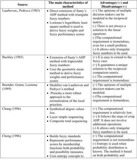
To discover the characteristics and advantages of proposed fuzzy MCDM model and fuzzy AHP a comparison between Main characteristics, advantages and disadvantages of different fuzzy AHP approaches (Tuysuz, Kahraman 2006) is implemented in Table 5.

Table 5: The comparison of different fuzzy AHP methods with proposed fuzzy MCDM

Source The main characteristics of method

Advantages (+) and Disadvantages (-)

Laarhoven,, Pedrycz (1983) Direct extension of Saaty’s

AHP method with triangular fuzzy numbers

Lootsma’s logarithmic least

square method is used to derive fuzzy weights and fuzzy performance scores

(+) The opinions of multiple decision makers can be modeled in the reciprocal matrix.

(-) There is not always a solution to the linear equations.

(-)The computational requirement is tremendous, even for a small problem. (-) It allows only triangular fuzzy numbers to be used.

Buckley (1985) Extension of Saaty’s AHP

method with trapezoidal fuzzy numbers

Uses the geometric mean

method to derive fuzzy weights and performance scores

(+) It is easy to extend to the fuzzy case.

(+) It guarantees a unique solution to the reciprocal comparison matrix. (-) The computational requirement is tremendous. Boender, Grann, Lootsma

(1989) Modifies van Laarhoven and Pedrycz’s method

 Presents a more robust

approach to the

normalization of the local priorities

(+) The opinions of multiple decision makers can be modeled.

(-)The computational requirement is tremendous.

Chang (1996) Synthetical degree values

low.

Layer simple sequencing

Composite total sequencing

(+) The computational requirement is relatively low. (+) It follows the steps of crisp AHP. It does not involve additional operations. (-) It allows only triangular fuzzy numbers to be used.

Cheng (1996) Builds fuzzy standards

Represents performance

scores by membership functions both probability and possibility measures.

Uses entropy concepts to

(+) The computational

(10)

calculate aggregate weights possibility measures.

Proposed Fuzzy MCDM Extension of rational model

Consensus rule based

Self optimization

Characterized for risk

analysis

Uses Euclidean distance to

find optimal solution

Pair-wise inconsistency

correction

(+) Uncertainty factors in group decision making are assessed by applying fuzzy logic

(+) Final solution is prioritized (+) Different fuzzy numbers and membership functions can be applied

(+) Experts can have inconsistent evaluation (+) Experts decision weight is efficiently applied to model (-) The computation

requirement is relatively high

5.0 CASE

STUDY

To illustrate the application of proposed fuzzy multi-criteria group decision making model in construction risk selection, we applied this model to a typical construction project as a case study.

Suppose a group of experts to identify inherent risk in a construction project consist of three experts P1, P2 and P3. To avoid complexity of manual computations, it is assumed that experts have same influence weights. Their weights, preference for risk factor selection and judgments for proposed assessment criteria are described in table 1, 3 and 4. The risk selection process by using proposed method is described as follow:

Stage 1: Alternatives, assessment criteria and influence weights generation

Step 1: to initiate the selection process, involved risks in project should be classified.

Each expert proposes one or more risk factor for project risk selection. Final alternative risk

S

is

determined by merging similar risk factors.



1, 2, 3, 4



S  S S S S

S1: Safety, S2: Scheduling, S3: Unavailability of resources, S4: Weather

Step 2: The experts should assess these risk factors with regard to magnitude and effect on project objectives by proposing an assessment criteria. In this case study we put emphasis on project duration and assess risk factors based on their impact on project duration. By merging overlapped criteria, five assessment criteria C1, C2, C3, C4 and C5 are obtained.

C1: Effect of new safety plans on project duration

C2: The impact of changing operations` scheduling on project delivery

C3: Change operations from non-critical to critical due to unavailability of resources C4: Consequence of undesired weather condition on project delays with regard to project

location.

C5: Impact of risk factor on costumer

Step 3: to avoid the complexity, we assume that all experts have same influence weights as ‘normal’.

Stage 2: Individual preferences generation

(11)

4 4 4

1 2 3

4

4 4 4

a a a

EI EI EI

a a a

EI EI EI

E E E EI a

a a a

EI EI EI

a a a

EI EI EI

           _ _  _ _                             _ _    _ _   _ _     

To correct the inconsistency of each pair-wise comparison matrix, the positive-transitive, De-In and In-De uncertainty rules are applied. Finalized pair-wise comparison matrices to express the possibility of selecting a risk factor, under certain criteria is as follow:

4 4 4 4

4 4 4

1 2 3

4

4 4 4 4

4 4 4

a a a a

EI EI EI EI

a a a

EI EI EI

E E E EI a

a a a a

EI EI EI EI

a a a

EI EI EI

         _ _  _ _                           _ _    _ _   _ _     

Normalized pair-wise comparison matrix and consistent weight for every assessment criteria are calculated by computing the geometric mean of every row.









4 4

1 2 3

4

1 1 1 ₄

1 2 3 3 3

2 2 2 4 4

1 2 3

4 4

3 3 3

1 2 3 4 4 ₄

4 4 4 4

1 2 3 ₃ ₃ ₄

5 5 5 ₄

10 4,6 10 10 4,6 10 10 4,6 10 a

w w w _a _x _x

w w w a a x x

a a x

w w w

a

w w w a

a

w w w _a

        _ _{  } _ _       _ _ _{ }       _ _ _{ } _ _       _ _ _{ }              _ _ _{ }       _ _ _{ }       _ _ _{ }       _ _        _{ } _













0 0 0

5 5 5

1 2 3

1 1 1

10 4,6 10 10 4,6 10

3

R R R

i i i

x

x x

w w w

                  _ _      



1 2 3

1 1 1 ₄

1 2 3

2 2 2 4

1 2 3

4

3 3 3

1 2 3 ₄

4 4 4

1 2 3 4

5 5 5

1 3

w w w _a

w w w a

a

w w w

a

w w w

a

w w w

      _{ }       _{ }       _{ }       _{ }          _{ }       _{ }       _{ }       _{ }                     

Step 5: To express the possibility of selecting a risk factor

( )

S

_i under criterion (Cj), three belief level matrices are obtained by group members:

1 1 1 1 1

11 12 13 14 15 ₄ ₁

1 1 1 1 1

21 22 23 24 25 7 4

1 1 1 1 1

4 1

31 32 33 34 35

1 1 1 1 1 ₁ ₄

41 42 43 44 45

,

b b b b b _M _{V L} _b _b

b b b b b V H M b b

b b M V L

b b b b b

b b

V L M

b b b b b

b   _ _{  }_ _ _{  }_   _ _ _ _   _   _ _   _     __{ } __ __{ } __   _ _{ }_ _    _   _{ }   _  

2 2 2 2 2

11 12 13 14 15 ₄ ₁

2 2 2 2 2

21 22 23 24 25 7 4

2 2 2 2 2

1 4

31 32 33 34 35

2 2 2 2 2 ₄ ₁

41 42 43 44 45

1

,

b b b b _M _{V L} _b _b

b b b b b V H M b b

b b V L M

b b b b b

b b

M V L

b b b b b

b   _ _{  }_ _ _{  }_   _ _ _ _   _   _ _   _     __{ } __ __{ } __   _ _{ }_ _    __ _{ } _{ }_ _{ } _  

3 3 3 3 3

1 12 13 14 15 ₁ ₄

3 3 3 3 3

21 22 23 24 25 4 7

3 3 3 3 3

4 1

31 32 33 34 35

3 3 3 3 3 ₄ ₁

41 42 43 44 45

.

b b b b _{V L} _M _b _b

b b b b b M V H b b

b b M V L

b b b b b

b b

M V L

b b b b b

(12)

Step 6: By applying the results obtained from step 4 to belief level matrix, three belief vectors are obtained as follow:

















































1 2 1 2 1 2 1 2

1 4 4 1 2 4 4 7 3 4 4 1 4 4 4 1

2 2 2 2 2 2 2 2

1 4 4 1 2 4 4 1 3 4 4 1 4 4 4 1

3 2 3 2 3 2 3 2

1 4 4 1 2 4 4 7 3 4 4 1 4 4 4 1

1 1 1 1

, , , ,

3 3 3 3

1 _, 1 _, 1 _, 1 _,

3 3 3 3

1 1 1 1

, , , .

3 3 3 3

b a a a b a a a b a a a b a a a

       

Stage 3: Group aggregation

Step 7: The normalized weight of decision makers denoted as follow:

0

1 2 3 1

3

1

1 2 3 4

1.2 1 1.2 R i i

v v v c

v

v v v a

          



Step 8: By applying obtained results from steps 6 and 7, weighted and normalized fuzzy decision vector is constructed:







 









 







2 2

1 2 3 2

1 1 1 2 1 3 1 4 4 1

2 2

1 2 3 2

2 1 2 2 2 3 2 4 4 7

1 2 3 2

3 1 3 2 3 3 3 4 4 1

1 1 ₁₀ _{4 , 6 10} ₁₀ _{4 , 8 20} _,

1.2 1.2

1 1 ₁₀ _{4 , 6 10} ₂₀ _{12 , 6 10} _,

1.2 1.2

1 1

10

1.2 1.2

r v b v b v b a a a x x x x

r v b v b v b a a a x

          _{ } _       __   ___   _  _{ } _       _   __   _           



 









 



2 2 2 2

1 2 3 2

4 1 4 2 4 3 4 4 4 1

4 , 6 10 10 4 , 8 20 ,

1 1

10 4 , 6 10 10 4 , 8 20 .

1.2 1.2

x x x

r v b v b v b a a a x x x x

 _ _ _{ } _ _ _        _{ } _       _   __   _   

Step 9: To reach the ideal solution, it is assumed that the ideal risk factor has minimum 0.25 and maximum 0.75 effect on project duration. The distances between obtained decision vector item for each risk factor and ideal risk factor are depicted below:

1

2

3

4

0.1536 ( )

0.0695 ( )

0.0725 ( )

0.1536 ( ) S S S S d Safety d Scheduling

d Unavailability of resources

d W eather

   

5.1 DISCUSSION OF RESULTS

By considering relative Euclidean distance, it is concluded that ‘scheduling’ risk factor has the most effect on project duration and ‘unavailability of resources’, ‘safety’ and ‘weather’ are on next order. Another conclusion that can be obtained from these results is the criticality and dependency of “Scheduling” and “Unavailability of resources”. As can be seen, “Unavailability of resources” has a closer distance to the most critical risk factor than “Safety” and “Weather” which shows a dependency between “Unavailability of resources” and “Scheduling”. Due to the dependency of these two risk factors, improving them should be done simultaneously. Otherwise improving one risk factor may lead to criticality of other.

(13)

For instance, he may re-arrange the float times or make revisions on critical paths. Also he may take into consideration the share activities that overlap the “Unavailability of resources”.

5.2 RESULT

COMPARISON

WITH FUZZY AHP

To discuss the difference between the proposed fuzzy MCDM and the fuzzy AHP, same case study has been implemented using Chang (1996) fuzzy AHP approach. Because of the advantages Chang’s extent analysis on fuzzy AHP are relatively superior to the others due to the reasons mentioned in Table 5, this method will be used in project risk evaluation (Tuysuz, Kahraman 2006). Because Chang`s approach allows only triangular fuzzy numbers, related non-triangular fuzzy numbers in case study, has been converted to non-triangular fuzzy numbers. After relatively high and time consuming computations, obtained results are as follow:

1 2 3 4

Risk Factor Scheduling

Risk Factor Unavailability of resources

Risk Factor Safety

Risk Factor W eather 

  

5.3 DISCUSSION

As concluded from this comparison, the priority rank of risk factors is same with proposed fuzzy MCDM method but the computations in utilized fuzzy AHP method is relatively high and limitation in applying other membership functions and fuzzy numbers rather than triangular fuzzy numbers, make it impractical in the field of construction risk assessment. Also there is no rational comparison between prioritized risk factors and as the result risk mitigation strategy cannot effectively be added to risk management process.

6.0 CONCLUSIONS

(14)

developing the programming solution for this model and utilizing other membership functions for complex problems.

REFERENCES

[1] Project Management Institute, (2008) A guide to the project management body of knowledge.

Project Management Institute Standards Committee.

[2] Perry, J.H. and Hayes, R.W. (1985) Risk and Its Management in Construction Projects,

Proceedings of the Institution of Civil Engineering, Part I, 78, 499-521.

[3] Abdou, O.A. (1996) Managing Construction Risks, Journal of Architectural Engineering,

2(1), 3-10.

[4] Shen, L.Y., Wu, G.W.C. and Ng, C.S.K. (2001) Risk Assessment for Construction Joint

Ventures in China, Journal of Construction Engineering and Management, 127(1), 76-81.

[5] Tah J.H.M and Carr V., A proposal for construction project risk assessment using fuzzy

logic,Construction Management and Economics (2000) 18, 491-500.

[6] Chapman R.J. (2001) The Controlling Influences on Effective Risk Identification and

Assessment for Construction Design Management, International Journal of Project Management, 19, 147-160.

[7] Shen, L.Y. (1997) Project Risk Management in Hong Kong, International Journal of Project

Management, 15(2), 101-105.

[8] Chen, H., Hao, G., Poon, S.W. and Ng, F.F. (2004) Cost Risk Management in West Rail

Project of Hong Kong, 2004 AACE International Transactions.

[9] Assaf, S. A. and Al-Hejji, S. (2006) Causes of delay in large construction projects,

International Journal of Project Management, 24(4), 349-357.

[10] Dikmen, I., Birgonul, M., Han, S., (2007) Using fuzzy risk assessment to rate cost overrun

risk in international construction projects, International Journal of Project Management, 25, 494–505.

[11] Zeng, J., An, M., and Smith, N. J. (2007) Application of a fuzzy based decision making