Statistical Methods for Time-Conditional Survival Probability and Equally Spaced Count Data

University of Pennsylvania

ScholarlyCommons

Publicly Accessible Penn Dissertations

1-1-2016

Statistical Methods for Time-Conditional Survival

Probability and Equally Spaced Count Data

Victoria Alexandria Gamerman

University of Pennsylvania, [email protected]

Follow this and additional works at:

http://repository.upenn.edu/edissertations

Part of the

Biostatistics Commons

This paper is posted at ScholarlyCommons.http://repository.upenn.edu/edissertations/1729

For more information, please [email protected].

Recommended Citation

Gamerman, Victoria Alexandria, "Statistical Methods for Time-Conditional Survival Probability and Equally Spaced Count Data" (2016).Publicly Accessible Penn Dissertations. 1729.

Statistical Methods for Time-Conditional Survival Probability and Equally

Spaced Count Data

Abstract

This dissertation develops statistical methods for time-conditional survival probability and for equally spaced

count data. Time-conditional survival probabilities are an alternative measure of future survival by accounting

for time elapsed from diagnosis and are estimated as a ratio of survival probabilities. In Chapter 2, we derive

the asymptotic distribution of a vector of nonparametric estimators and use weighted least squares

methodology for the analysis of time-conditional survival probabilities. We show that the proposed test

statistics for evaluating the relationship between time-conditional survival probabilities and additional time

survived have central Chi-Square distributions under the null hypotheses. Further, we conducted simulation

studies to assess the empirical probability of making a type I error for one of the hypotheses tests developed

and to assess the power of the various models and statistics proposed. Additionally, we used weighted least

squares techniques to fit regression models for the log time-conditional survival probabilities as a function of

time survived after diagnosis to address clinically relevant questions. In Chapter 3, we derive the asymptotic

distribution of time-conditional survival probability estimators from a Weibull parametric regression model

and from a Logistic-Weibull cure model, adjusting for continuous covariates. We implement the weighted

least squares methodology to assess relevant hypotheses. We create a statistical framework for investigating

time-conditional survival probability by developing additional methodological approaches to address the

relationship between estimated time-conditional survival probabilities, time survived, and patient prognostic

factors. Over-dispersed count data are often encountered in longitudinal studies. In Chapter 4, we implement

a maximum-likelihood based method for the analysis of equally spaced longitudinal count data with

over-dispersion. The key features of this approach are first-order antedependence and linearity of the conditional

expectations. We also assume a Markovian model of first order, implying that the value of an outcome on a

subject at a specific measurement occasion only depends on the value at the previous measurement occasion.

Our maximum likelihood approach using the Poisson model for count data benefits from a simple

interpretation of regression parameters, like that in GEE analysis of count data.

Degree Type

Dissertation

Degree Name

Doctor of Philosophy (PhD)

Graduate Group

Epidemiology & Biostatistics

First Advisor

Phyllis A. Gimotty

STATISTICAL METHODS FOR TIME-CONDITIONAL SURVIVAL PROBABILITY AND EQUALLY SPACED COUNT DATA

Victoria A. Gamerman

A DISSERTATION

in

Epidemiology and Biostatistics

Presented to the Faculties of the University of Pennsylvania

in

Partial Fulfillment of the Requirements for the

Degree of Doctor of Philosophy

2016

Supervisor of Dissertation Co-Supervisor of Dissertation

Phyllis A. Gimotty Justine Shults

Professor of Biostatistics Professor of Biostatistics

Graduate Group Chairperson

John H. Holmes, Professor of Medical Informatics in Epidemiology

Dissertation Committee

Susan Ellenberg, Professor of Biostatistics

STATISTICAL METHODS FOR TIME-CONDITIONAL SURVIVAL PROBABILITY AND EQUALLY

SPACED COUNT DATA

c

COPYRIGHT

2016

Victoria A. Gamerman

This work is licensed under the

Creative Commons Attribution

NonCommercial-ShareAlike 3.0

License

To view a copy of this license, visit

ACKNOWLEDGEMENT

I would like to acknowledge the support of my committee and thank the Biostatistics faculty and my

ABSTRACT

STATISTICAL METHODS FOR TIME-CONDITIONAL SURVIVAL PROBABILITY AND EQUALLY

SPACED COUNT DATA

Victoria A. Gamerman

Phyllis A. Gimotty

Justine Shults

This dissertation develops statistical methods for time-conditional survival probability and for equally

spaced count data. Time-conditional survival probabilities are an alternative measure of future

sur-vival by accounting for time elapsed from diagnosis and are estimated as a ratio of sursur-vival

probabil-ities. In Chapter 2, we derive the asymptotic distribution of a vector of nonparametric estimators and

use weighted least squares methodology for the analysis of time-conditional survival probabilities.

We show that the proposed test statistics for evaluating the relationship between time-conditional

survival probabilities and additional time survived have centralχ2-distributions under the null hy-potheses. Further, we conducted simulation studies to assess the empirical probability of making

a type I error for one of the hypotheses tests developed and to assess the power of the various

models and statistics proposed. Additionally, we used weighted least squares techniques to fit

re-gression models for the log time-conditional survival probabilities as a function of time survived after

diagnosis to address clinically relevant questions. In Chapter 3, we derive the asymptotic

distribu-tion of time-condidistribu-tional survival probability estimators from a Weibull parametric regression model

and from a Logistic-Weibull cure model, adjusting for continuous covariates. We implement the

weighted least squares methodology to assess relevant hypotheses. We create a statistical

frame-work for investigating time-conditional survival probability by developing additional methodological

approaches to address the relationship between estimated time-conditional survival probabilities,

time survived, and patient prognostic factors. Over-dispersed count data are often encountered

in longitudinal studies. In Chapter 4, we implement a maximum-likelihood based method for the

analysis of equally spaced longitudinal count data with over-dispersion. The key features of this

approach are first-order antedependence and linearity of the conditional expectations. We also

specific measurement occasion only depends on the value at the previous measurement occasion.

Our maximum likelihood approach using the Poisson model for count data benefits from a simple

TABLE OF CONTENTS

ACKNOWLEDGEMENT . . . iii

ABSTRACT . . . iv

LIST OF TABLES . . . viii

LIST OF ILLUSTRATIONS . . . ix

CHAPTER 1 : INTRODUCTION . . . 1

1.1 Time-Conditional Survival Probability Methods . . . 1

1.2 Longitudinal Count Data Methods . . . 7

1.3 Dissertation Structure . . . 9

CHAPTER 2 : NONPARAMETRICTIME-CONDITIONALSURVIVALPROBABILITY . . . 10

2.1 Introduction . . . 10

2.2 Estimation of Time-Conditional Survival Probabilities . . . 12

2.3 Distribution Theory . . . 13

2.4 Hypothesis Testing Using Weighted Least Squares . . . 17

2.5 Simulation Studies . . . 28

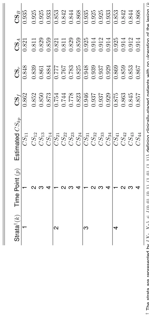
2.6 Application: Staging Procedure and Time-Conditional Survival Probability for Stage II Melanoma Patients . . . 34

2.7 Discussion . . . 48

CHAPTER 3 : PARAMETRIC TIME-CONDITIONALSURVIVALPROBABILITY . . . 55

3.1 Introduction . . . 55

3.2 Parametric Time-Conditional Survival . . . 55

3.3 An Example: The Weibull Distribution . . . 65

3.4 Application to Real-World Data . . . 69

CHAPTER 4 : ANALYSIS OF LONGITUDINAL COUNT DATA WITH SPECIFIED MARGINAL

MEANS AND FIRST-ORDERANTEDEPENDENCE. . . 93

4.1 Introduction . . . 93

4.2 Methods . . . 95

4.3 Application . . . 99

4.4 Simulation Studies . . . 103

4.5 Discussion . . . 105

CHAPTER 5 : DISCUSSION. . . 114

APPENDICES . . . 118

LIST OF TABLES

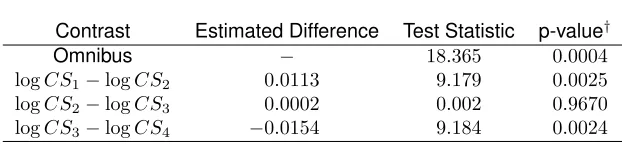
TABLE 2.1 : SEER melanoma contrasts of profile-based differences . . . 51

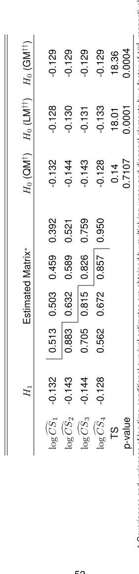
TABLE 2.2 : Estimates of log time-conditional melanoma-specific survival probabilities,

their variance-covariance matrix, and estimates from the saturated (H1),

QM, LM, and GM models . . . 52

TABLE 2.3 : Parameter estimates for the multivariable analysis . . . 53

TABLE 2.4 : Estimates of time-conditional melanoma-specific survival probabilities from the multivariable analysis . . . 54

TABLE 3.1 : Maximum likelihood estimates of the Weibull survival distribution for

disease-specific survival of esophageal cancer patients adjusting for tumor length. . 88

TABLE 3.2 : Maximum likelihood estimates of the Weibull mixture cure model for disease-specific survival. . . 89

TABLE 3.3 : Estimated covariance matrix∗ _{for the time-conditional survival probability}

from the Weibull mixture cure model for disease-specific survival. . . 90

TABLE 3.4 : Estimates of 5-year time-conditional survival probability from the Weibull mixture cure model for disease-specific survival adjusting for fixed gender (male), fixed age at diagnosis (60 years), fixed tumor thickness (3.58 mm) and varying staging type (clinical versus pathological), number of nodes ex-amined, and ulceration status along with the estimated covariance and cor-relation matrices for the alternative hypothesis. . . 91 TABLE 3.5 : Change in 5-year time-conditional survival probability given 1 and given

10 years after diagnosis from the Weibull mixture cure model for disease-specific survival with Bonferroni adjustment. . . 92

TABLE 4.1 : Estimated parameters from the ML, GEE, and Poisson models in the analy-sis of the doctor visits data. . . 107 TABLE 4.2 : Mean and variance for the placebo and treatment groups. . . 108 TABLE 4.3 : Estimated parameters from the GEE and ML approaches for analysis of the

epilepsy data when Period is included in the models. . . 109 TABLE 4.4 : Estimated parameters from the GEE and ML approaches for analysis of the

epilepsy data when Period is not included in the models. . . 110 TABLE 4.5 : Small sample efficiencies for evaluating the AR(1) correlation structure for

varying values ofαand sample size per group. . . 111 TABLE 4.6 : Percent bias for evaluating the AR(1) correlation structure for varying values

ofαand sample size per group. . . 112 TABLE 4.7 : Coverage probabilities for the ML and GEE approaches with the AR(1)

cor-relation structure for varying values ofαand sample size per group. . . 113

TABLE B.1 : Maximum likelihood estimates from four Weibull mixture cure models for disease-specific survival. . . 136 TABLE B.2 : Results from the likelihood ratio test for nested models. . . 137 TABLE B.3 : Estimates of 5-year time-conditional survival probability from four Weibull

mixture cure models for disease-specific survival adjusting for fixed tumor thickness (3.58mm) and varying ulceration status. . . 138

LIST OF ILLUSTRATIONS

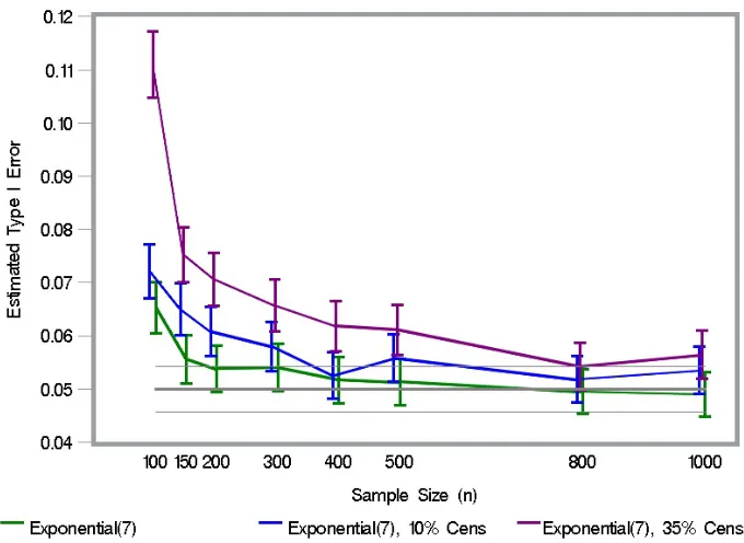
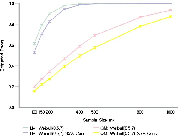
FIGURE 2.1 : Expected type I error of 5% with the 95% confidence interval for 10,000 datasets and estimated type I error for the GM model test statistic (and 95% confidence intervals) for no censoring, 10%, and 35% uniform random censoring. . . 31 FIGURE 2.2 : Estimated power for the LM and QM test statistics with and without censoring. 32

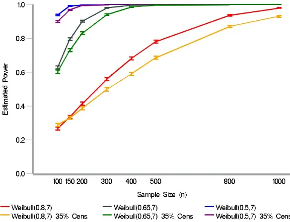
FIGURE 2.3 : Estimated power for the GM model test statistic. . . 33

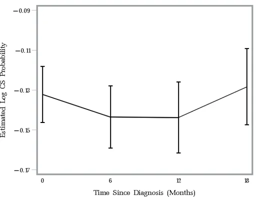
FIGURE 2.4 : Nonparametric Kaplan-Meier estimated 3-year log time-conditional survival probabilities given 0, 6, 12, and 18 months after diagnosis for Stage II patients. . . 37 FIGURE 2.5 : Nonparametric Kaplan-Meier estimated 3-year log time-conditional survival

probabilities given 0, 6, 12, and 18 months after diagnosis for patients by procedure: (1) Pathologically staged (some nodal procedure) and (2) Clin-ically staged (no nodal procedure). . . 39 FIGURE 2.6 : Nonparametric Kaplan-Meier estimated 3-year log time-conditional survival

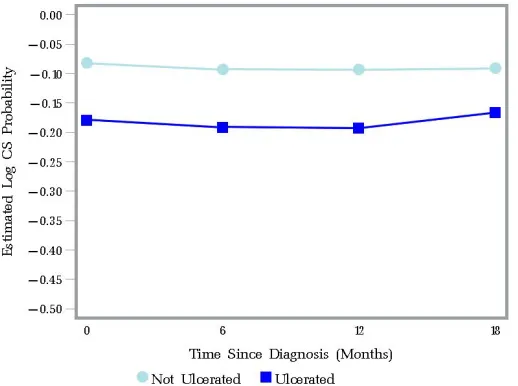
probabilities given 0, 6, 12, and 18 months after diagnosis for patients by ulceration status: (1) Not ulcerated and (2) Ulcerated. . . 39 FIGURE 2.7 : Nonparametric Kaplan-Meier estimated 3-year log time-conditional survival

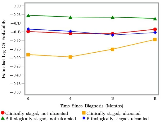
probabilities given 0, 6, 12, and 18 months after diagnosis for patients in one of four groups: (1) Pathologically staged (some procedure) and not ulcerated, (2) Pathologically staged (some procedure) and ulcerated, (3) Clinically staged (no nodal procedure) and not ulcerated, and (4) Clinically

staged (no nodal procedure) and ulcerated. . . 43

FIGURE 3.1 : The unadjusted survival estimate from the parametric Weibull distribution and the empirical Kaplan-Meier survival function for the SEER esophageal sample. . . 70 FIGURE 3.2 : Estimated 5-year time-conditional survival probability given increasing time

survived for mean tumor length from the Weibull distribution based on the

SEER esophageal sample. . . 71

FIGURE 3.3 : Estimated 5-year time-conditional survival probability, given that survival is greater than 1, 2, and 3 years after diagnosis, for increasing tumor length

from the Weibull distribution based on the SEER esophageal sample. . . 72

FIGURE 3.4 : Estimated 5-year time-conditional survival probability given increasing time survived for tumor length at 2, 5, 10, and 15 cm from the Weibull distribution

based on the SEER esophageal sample. . . 73

FIGURE 3.5 : Estimated time-conditional survival probability, given that survival is greater

than 2 years after diagnosis, as a function of∆evaluated at mean tumor

length from the Weibull distribution based on the SEER esophageal sam-ple. . . 74 FIGURE 3.6 : Estimated 2-, 3-, 4-, and 5-year time-conditional survival probability, given

that survival is greater than 2 years after diagnosis, for increasing tumor length from the Weibull distribution based on the SEER esophageal sam-ple. . . 75

FIGURE 3.7 : Empirical survivor function for the SEER melanoma sample. . . 77

FIGURE 3.8 : Estimated 5-year time-conditional survival for the SEER melanoma sample

CHAPTER 1

I

This dissertation develops statistical methods for time-conditional survival probability and for equally

spaced count data. In Chapter 2, we derive the asymptotic distribution of a vector of nonparametric

estimators and use weighted least squares methodology for the analysis of time-conditional

sur-vival probabilities. In Chapter 3, we derive the asymptotic distribution of time-conditional sursur-vival

probability estimators from a Weibull parametric regression model and from a Logistic-Weibull cure

model, adjusting for continuous covariates. We implement the weighted least squares methodology

to assess relevant hypotheses. In Chapter 4, we implement a maximum-likelihood based method

for the analysis of equally spaced longitudinal count data with over-dispersion.

1.1. Time-Conditional Survival Probability Methods

This work was motivated by increased attention in the medical literature on conditional survival. We

distinguish between two types of conditional survival probabilities. The first refers to those

proba-bilities that condition on fixed covariates at time of diagnosis (e.g., Xu and O’Quigley, 2000). The

second, which we refer to as time-conditional survival probabilities, condition on time survived and

will be the focus of the work here. With earlier detection, better therapies for diseases, and more

systematic tracking, patients in recent years have been surviving longer and information on their

long-term follow-up is more readily available. With patients living longer, there is interest in

estimat-ing the probability of survival not from a patient’s time of diagnosis, but rather from her/his present

state sometime after diagnosis. Time-conditional survival probability is defined as the probability

of surviving at least an additional ∆ years given that a patient has already surviveda years. As

described in further detail in Chapter 2, this probability can be estimated by the ratio of thea- and (∆ +a)-year estimated survival probabilities from a single Kaplan-Meier survivor function (Kaplan and Meier, 1958).

We create a statistical framework for investigating time-conditional survival probability by

devel-oping additional methodological approaches to address the relationship between estimated

time-conditional survival probabilities, time survived, and patient prognostic factors. While the work

disciplines.

1.1.1. Nonparametric Methods

Time-to-event data generally contain observations that are censored. Censoring occurs in

situa-tions when a patient has not yet experienced an event and is known to be alive up to a particular

time. When all that is known is that a patient is alive at a given point in time, that patient’s survival

data is right censored. In this work, we use the survival function, defined as the probability of

surviv-ing beyond a specified time, to estimate time-conditional survival probability. For the nonparametric

approach, the Kaplan-Meier Product-Limit methodology is used to estimate the survivor function,

which is then used to estimate survival probabilities (Kaplan and Meier, 1958).

Time-conditional survival probabilities are an alternative measure of future survival by accounting

for time elapsed from diagnosis and are estimated as a ratio of survival probabilities. Relative

survival is also defined as a ratio of probabilities in a target population relative to the expected

survival probability in a comparable general population over a given follow-up period (Dickman and

Adami, 2006). The estimate of five-year relative survival is the ratio of the estimated five-year

sur-vival probability for the target population divided by the expected five-year sursur-vival probability in the

general population that is assumed to be fixed (e.g., Ederer, Axtell, and Cutler, 1961; Hakulinen,

1982). Dickman et al., 2004 describe four approaches to estimate a regression model for relative

survival using maximum likelihood methodology. In our work, we use the weighted least squares

methodology to analyze nonparametric and parametric based estimators of time-conditional

sur-vival probabilities.

Over the last two decades, clinical investigators have presented point estimates and

correspond-ing 95% confidence limits for time-conditional survival probabilities. Clinical investigators report

that patients who have survived for some time beyond diagnosis are more interested in estimates

of time-conditional survival probabilities because these estimates offer more relevant prognostic

information than estimates from traditional survival probabilities computed using time from initial

diagnosis (e.g., Xing et al., 2010). Clinical research publications increasingly present estimates

of time-conditional survival probabilities. A topic search for “conditional survival” on Web of

Sci-ence conducted in early 2015 revealed approximately 150 articles published in the past five years

ar-ticles published in 2000–2004. The interest in these estimates demonstrates its strong relevance

to many clinical settings and highlights the importance of developing modeling methodology for

time-conditional survival probabilities.

In Chapter 2, we develop the asymptotic distribution for estimates of log time-conditional survival

probabilities. The asymptotic distribution facilitates the extension of statistical tools from estimation

to the statistical testing of different hypotheses of interest. We base our methods for hypothesis

testing and model fitting on the work of Grizzle, Starmer, and Koch, 1969, who used weighted least

squares as part of a regression modeling strategy for proportions and proposed test statistics for

evaluating simplified models. Koch, Johnson, and Tolley, 1972 applied this approach to survival

probabilities. With modifications, we apply their approach to time-conditional survival probabilities.

We use weighted least squares to develop a test statistics for relevant hypotheses, e.g. a

multivari-ate omnibus test of pairwise differences. We show that the proposed test statistics for evaluating

the relationship between time-conditional survival probabilities and additional time survived have

centralχ2_{-distributions under the null hypotheses. Further, we conducted simulation studies to}

as-sess the empirical probability of making a type I error for one of the hypotheses tests developed

and to assess the power of the various models and statistics proposed.

Additionally, we used weighted least squares techniques to fit regression models for the log

time-conditional survival probabilities as a function of time survived after diagnosis to address clinically

relevant questions. Quadratic, linear, and global mean models are used to explore the relationship

between log time-conditional survival probabilities and time survived. To include discrete,

categori-cal covariates, we develop a parametric framework for multivariable models. To avoid the problem

of multiple testing due to comparisons among covariate patterns resulting from either categorical

variables or categorization of continuous variables (Bennette and Vickers, 2012), we propose an

overall test of significance in addition to pairwise comparisons. Population based survival data from

patients with melanoma are used to illustrate the proposed methodology by evaluating survival in

patients who underwent clinical staging versus pathological staging (Balch et al., 2001).

In contrast, consider an alternative approach for nonparametric inference using median residual

lifetimes with censoring proposed by Jeong, Jung, and Costantino, 2008. As with time-conditional

survival probabilities, they draw the comparison between information at diagnosis and at a time

and the impact of first-line treatment on life expectancy fromdiagnosisin contrast with a patient’s

interest in their estimate of residual life expectancy sometime after diagnosis and the impact of

additional, second-line treatment.

To obtain an estimate of median residual lifetime for censored survival data, the authors’ first model

the survivor function. Then their approach infers the median of remaining lifetimes among survivors

beyond time t at a fixed time point, t0, to obtain an estimate of the median residual life function

evaluated att0. To compute the median residual lifetime, the authors compute the residual lifetime

for a patient who has survived beyondt0asS(t|t0) =S(t+t0)/S(t0)fort0 ≥0. As given in their

manuscript by Equation 2, they then obtain the estimated median of the residual lifetime distribution

att0by solving the equationuˆ(θt0) = 0forθt0 where

ˆ

u(θt0) = ˆS(t0−θt0)−0.5 ˆS(t0),

and whereSˆ(t)is the Kaplan-Meier estimator ofS(t)(Jeong, Jung, and Costantino, 2008).

The resulting estimate provided to patients and physicians is the median residual life in years, which

is more intuitive for patients to understand than a survival probability. However, a limitation of this

approach is the influence of the proportion of censored observations as the median failure time

cannot be theoretically defined until the minimum of the survival curve reaches 0.5 (Jeong, Jung,

and Costantino, 2008). This issue is addressed in the later work by Park, Jeong, and Lee, 2012.

As will be demonstrated in the application of Chapter 2, time-conditional survival probability under

the nonparametric Kaplan-Meier framework is advantageous as it can be estimated irrespective of

the minimum of the survival curve.

Further, in their paper, Jeong, Jung, and Costantino, 2008 note that the methods of comparing

median residual life functions over the entire follow-up period that they developed did not address

issues of multiple comparisons. In our work, we developed an omnibus test of contrasts and other

hypotheses tests along with providing estimators of the covariance matrix to allow researchers to

address issues of multiple comparisons. Lastly, the authors note the need for future research to

develop a regression model that would take into account continuous prognostic factors and develop

such an approach using regression on quantile residual life (Jung, Jeong, and Bandos, 2009). This

Kaplan-Meier framework in Chapter 2 and extended the approach to allow for continuous covariates

in the parametric framework in Chapter 3.

1.1.2. Parametric Survival Methods

Parametric models are used by researchers for time-to-event data in the estimation of model

param-eters and related functions such as the parametric hazard function. Modeling survival time without

the inclusion of covariates provides an estimate of the survival experience on the assumption that

the underlying population is homogeneous. Incorporating covariates allows for the study of

het-erogeneous populations that may characterize observational studies based in disease registries,

rather than populations from clinical trials with strict inclusion and exclusion criteria. Covariates

can be incorporated by modeling the natural logarithm of survival time (e.g., Weibull or log logistic

regression models) or using an accelerated failure-time model. In both cases, when the parametric

model provides a good fit for the data, the estimates from the model are often more precise than

those from the nonparametric setting because they are based on fewer parameters (e.g., Lambert

and Royston, 2009).

In Chapter 2, we develop the large sample distribution for log time-conditional survival and pairwise

tests for differences among a set of estimates. We also use weighted least squares to model a

profile of estimates as a function of time survived and compare time-conditional survival estimates

across groups of patients. Stratifying patients into groups based on covariate patterns requires

using categorical variables or categorizing continuous variables. For example, Barchielli et al.,

1994 categorized age at time of diagnosis into 5-year groups to evaluate the prognostic effect of

this variable as opposed to evaluating it as a continuous covariate. Stratification assumes that

patients falling into one stratum are homogeneous and, therefore, have a homogeneous risk for the

outcome (Bennette and Vickers, 2012). However, ignoring variability within the stratum leads to a

loss of information and reduces the power of a test of association (Greenland, 1995). Therefore,

we extend the work in Chapter 2 by developing methods under parametric assumptions.

Chapter 3 develops methods for parametric time-conditional survival probability. It extends the

methodology of Chapter 2 by allowing for the inclusion of multiple covariates, including continuous

variables, in a single regression model for time-conditional survival probability. Two regression

is based on the log-linear model for the relationship between time survived from diagnosis and

covariates of interest. It is important to note that a survival model that tends to zero with increasing

time after diagnosis will be appropriate for a disease with a generally poor prognosis. If, on the

other hand, long-term survival is of interest due to patients surviving longer and having improved

prognoses, a model that allows for a non-zero probability of indefinite survival or cure will better

fit the data. The second regression is a parametric cure model where the underlying population

is a mixture of patients who experience the event of interest and those who do not. The Weibull

distribution is used to illustrate the methods which are applied to esophageal cancer data (Weibull

regression model with covariates) and to melanoma data (Logistic-Weibull cure model).

A recent paper by Hieke et al., 2015 emphasized the usefulness of the conditional survival concept

to provide information on the evolution of prognosis over time. In their application, these authors

used Kaplan-Meier survival estimation to analyze data from multiple myeloma patients stratified by

age groups and disease stage. Further, while they stated that methods to estimate conditional

sur-vival exist using Kaplan-Meier and Cox regression, they did not note uses of parametric regression

models in the estimation of conditional survival. This indicates that a methodological gap remains

in nonparametric estimation adjusting for continuous covariates which can be addressed using a

parametric statistical approach.

When assessing hypothesis testing based on conditional survival methods, Hieke et al., 2015 show

estimates in Figure 2B with a 5-year conditional survival profile plotted for each age strata and

95% confidence intervals around each point estimate of time since diagnosis in years. In our

work, we develop nonparametric and parametric methods that account for the correlation among

time-conditional survival probabilities through the hypothesis testing framework by incorporating the

covariance matrix into the test statistic.

Parast, Cheng, and Cai, 2011, 2012 have developed methodology for incorporating short-term

out-come information to predict long-term disease outout-comes where the long-term event of interest is

time to a terminal event such as death and the short-term event is time to a non-terminal event.

These authors propose methods for incorporating censored short-term event information to

pre-dict long-term survival beyond the parametric models in a multi-state survival setting, which may

lead to invalid prediction if the model assumptions do not hold. In their earlier work (2011) they

and information on a discrete marker. However, similar to the limitation in the time-conditional

sur-vival methods developed in Chapter 2, these methods cannot account for information from one or

more continuous covariates. The authors then extended work by others and proposed a flexible

ap-proach that allows for the inclusion of longitudinal predictor information collected such as repeated

biomarker measurements (2012). As the authors note, including information about a short-term

outcome in addition to genetic or biomarker measurements may lead to an improved ability to

pre-dict long-term survival. Accordingly, future research on implementing competing risks models in

the estimation of time-conditional survival needs to be explored.

1.2. Longitudinal Count Data Methods

Longitudinal count data are often encountered in scientific studies. Common features of longitudinal

count data include intra-subject correlation and over-dispersion. Intra-subject correlation is due to

similarities between the repeated measurements on each participant. When the variance is larger

than expected for the assumed distribution of the outcome variable then over-dispersion is observed

(Efron, 1992).

As noted by Farewell and Farewell, 2012, one approach to modeling longitudinal Poisson count

data is using a generalized linear mixed model with Poisson distributions conditional on random

effects. They note that a marginal modeling approach may be preferred for cases where the effect of

explanatory variables at the population-averaged level (marginal effects) is of interest as opposed to

subject-specific effects. Heagerty and Kurland, 2001 showed that marginal modeling is more robust

for the estimation of regression parameters as compared to subject-specific covariate effects when

there is a departure from the underlying random effects structure.

Marginal modeling can be implemented using generalized estimating equation (GEE) methods

(Solis-Trapala and Farewell, 2005). Two considerations when using the GEE approach are that

GEE methods do not give the researcher an understanding of the sources of variation and,

un-like parametric maximum un-likelihood estimation, there is reduced efficiency (Farewell and Farewell,

2012). Given these limitations, Farewell and Farewell, 2012 developed methods to analyze such

data using the Dirichlet negative multinomial distribution. From their simulation study to evaluate the

model robustness and finite-sample behavior, the authors found that the Dirichlet negative

data, Farewell and Farewell, 2012 also fit a Poisson generalized linear mixed model and found that

the estimated coefficients and standard errors were similar to their Dirichlet negative multinomial

model. Our approach offers an alternative to their methods and to the GEE approach.

Over-dispersed count data are often encountered in longitudinal studies. This may be present in

the context of the number of patients with epileptic seizures (Farewell and Farewell, 2012; Thall

and Vail, 1990) or the number of patients who had transplants performed. Over-dispersion occurs

when the variability is larger than the standard Poisson variability that is expected. However, few

likelihoods are available for the simulation and analysis of such data (Efron, 1992). Therefore, we

provide a maximum likelihood approach to model longitudinal Poisson count outcomes.

In Chapter 4, we develop an approach for maximum likelihood analysis of longitudinal discrete data

with over-dispersion. We implement a likelihood proposed for simulation of over-dispersed random

variables with specified marginal means and product correlations by Guerra and Shults, 2014.

The key features of this approach are first-order antedependence and linearity of the conditional

expectations. We also assume a Markovian model of first order, implying that the value of an

outcome on a subject at a specific measurement occasion only depends on the value at the previous

measurement occasion. Our maximum likelihood approach using the Poisson model for count data

benefits from a simple interpretation of regression parameters, like that in GEE analysis of count

data.

As described elsewhere (e.g., Shults et al., 2006 Appendix A), the maximum likelihood approach

for count data requires information on the correlation between adjacent measurements on each

subject. While Guerra and Shults, 2014 developed general simulation methods allowing for different

patterns of correlation, we focus our maximum likelihood approach to Poisson count data with a

first-order autoregressive (AR(1)) correlation structure. Given the specified marginal means and

adjacent correlations, the AR(1) correlation structure is induced and the marginal distributions are

over-dispersed relative to the Poisson distributions. Under the AR(1) structure, it is assumed that

the adjacent intra-subject correlations are constant. This assumption is appropriate when it is

reasonable to assume that two count outcomes that are measured closer in time will be more

highly correlated, because they are assumed to be more similar, rather than if they are farther apart

We obtain likelihood-based estimating equations for the regression and correlation parameters.

Simulations are conducted to demonstrate that the approach has good statistical properties. This

approach is applied to the analysis of health policy data on doctor visits (StataCorp LP, 2013;

Winkelmann, 2004) and to seizure data (Farewell and Farewell, 2012; Thall and Vail, 1990).

1.3. Dissertation Structure

This dissertation is structured as follows. Chapter 2 defines the framework for nonparametric

meth-ods to assess time-conditional survival probability. This includes the development of the

asymp-totic distribution for a vector or profile of time-conditional survival probabilities, a flexible

frame-work for hypothesis testing using point estimates, and regression modeling to address clinically

relevant questions. Chapter 3 builds a parametric framework for time-conditional probability and

incorporates multiple discrete and continuous covariates in modeling time-conditional survival

pro-files. These methods are applied using a Weibull regression model for data where survival tends

to zero with increasing time after diagnosis and a Logistic-Weibull cure model for data where there

is evidence of cure in a fraction of patients. Chapter 4 discusses a new approach for maximum

likelihood-based analysis of correlated count data with over-dispersion. This maximum likelihood

approach assesses the problem of over-dispersion in Poisson data with an AR(1) structure. Such

longitudinal outcomes can be found in medical research in situations where measurements on a

subject are captured at pre-specified occasions over time. Poisson regression is often used for

analysis of count data, but would not be appropriate in an analysis of data characterized by

over-dispersion. Key assumptions of the maximum likelihood approach include the first-order Markov

property and the linearity of the conditional expectations for the conditional distributions. The

pro-posed approach is applied in analysis of data on doctor visits and epilepsy seizure data (R code is

CHAPTER 2

N

T

-C

S

P

2.1. Introduction

Commonly reported statistics for cancer patients include estimates of survival and conditional

sur-vival probabilities. Over the past two decades, clinical investigators have also reported estimated

time-conditional survival probabilities for patients who have already survived for a specified amount

of time after the diagnosis or therapy of their disease. While conditional survival probabilities

condi-tion on covariates that were measured at the time of diagnosis (e.g., Xu and O’Quigley, 2000),

time-conditional survival probabilities condition on the time already survived after diagnosis. Specifically,

time-conditional survival probability is defined as the probability of surviving at least an additionalx

years given survivalayears after diagnosis.

Typically, what is reported in the medical literature are the point estimates of the time-conditional

survival probabilities and their associated 95% confidence limits that are based on the estimated

Kaplan-Meier survival function (e.g., Choi et al., 2008; Merrill, Henson, and Ries, 1998; Xing et al.,

2010). These estimates can be used to answer questions such as “What is the expected probability

that a patient will survive an additional 5 years, given that she has already survived 5 years since

diagnosis”? However, additional methods are needed to answer other clinically relevant questions

of interest, such as “Does the expected probability that a patient will survive an additional 5 years

significantlyincrease with increasing time post-diagnosis”? For example, is the expected probability

of an additional 5 years survival significantly greater if the patient has survived 5 years than if she

has only survived 1 year after diagnosis?

This type of question is of clinical interest because it has been observed (Ries et al., 2003) that

for some cancers, the estimated time-conditional survival probabilities increase with an increasing

number of years survived. More recently, Miller, Lynch, and Buckwalter, 2013 investigated 5-year

conditional survival for a cohort of patients from the Surveillance, Epidemiology, and End Results

(SEER) registry with osteosarcoma and Ewings sarcoma. They found that 5-year conditional

sur-vival was 74.8% at diagnosis and 91.4% given sursur-vival beyond 5 years after diagnosis. Wang et al.,

from the SEER registry. For Stage I patients, the 5-year survival at diagnosis was 71% and 5-year

conditional survival given survival beyond 5 years increased to 74%.

New methods are also needed to address questions about trends in the time-conditional survival

probabilities over the course of a study. For patients who have survived some time after diagnosis,

the probability of surviving an additional number of years may be different from an initial overall

survival probability at diagnosis because the probability is not necessarily static (Choi et al., 2008).

For example, is the change in probabilities linear, or quadratic? If we have different sub-groups

of patients, does the change over time differ between the groups? Does the strength of this

rela-tionship differ for males versus females? In this chapter we develop methodology to answer such

questions.

In Section 2, we define point estimates of time-conditional survival probabilities and their 95%

confidence intervals, methods which have been published in the medical literature. In Section 3, we

develop the asymptotic distribution of a vector of estimators of time-conditional survival probabilities

using large sample distribution theory. We derive the estimate for the natural logarithm (log) of

time-conditional survival probability and its estimated variance as a function of the number of years

survived.

Grizzle, Starmer, and Koch, 1969 presented a general approach for the analysis of categorical

data using linear models with weighted regression. This approach allowed for simplification in

model formulation and hypothesis testing within the linear models framework. Koch, Johnson,

and Tolley, 1972 applied linear regression models and weighted least squares methodology to the

analysis of survival rates. In Section 4, we use Koch’s regression modeling strategy using weighted

least squares to analyze time-conditional survival probabilities. In particular, we develop Wald test

statistics (Wald, 1943) to evaluate trends in time-conditional survival estimators that are relevant to

patients, clinicians, and researchers.

In Section 5, we present results from simulations that assess power and the empirical probability of

making a type I error for particular tests. We then apply the proposed methodology to a cancer study

in Section 6, where we estimate time-conditional probabilities for melanoma patients as a function

of time survived. Additionally, we evaluate the differences in time-conditional survival between

2.2. Estimation of Time-Conditional Survival Probabilities

2.2.1. Notation

Letnbe the fixed number of individuals in a study. DefineTi = min(Xi, Ci), whereXi andCiare

the event and censoring times for theith subject, respectively. We assume the censoring time,Ci,

is independent of the event time,Xi. We observe the pair(ti, δi), i= 1, . . . , n, wheretiis the time

on study andδi=I(Xi≤Ci)is the indicator variable for whethertiis an event or a censoring time.

DefineJ distinct event times to bet(1) <· · ·< t(J)allowing for possible ties in the data. For each

observed event timet(j) in the set of ordered event times, definenj to be the number of subjects

at risk at timet(j)and letdj be the number of events observed at timet(j)among thenj subjects

at risk. To incorporate information on censoring, letwjdenote the number of observations that are

(right) censored at times after thejth event time, but prior to the(j+ 1)th time.

2.2.2. Current approach

Assume we have non-informative censoring, where knowledge of an individual’s censoring time

provides no further information about the patient’s likelihood of survival at a future time had they

continued on the study. Under this assumption of non-informative censoring, the likelihood is given

by

L(π1, . . . , πN)∝ J Y

j=1 πdj

j S(t(j−1))djS(t(j))wj,

whereπj = lim

∆t↓0P(t

−

(j) < T ≤t

−

(j)+ ∆t|T > t

−

(j))is the conditional probability of an event att(j), j = 1, . . . , J, and where the survival function is given by S(t) = P(T ≥t)such thatt(0) = 0and S(t(0)) = 1(Lachin, 2000).

Survival beyond timet(j) requires a subject to be event-free beyond timet(j−1) and all previous

times. If the survivor function is rewritten in terms of πj, the likelihood can be simplified in the

following product binomial form

L(π1, . . . , πJ)∝ J Y

j=1 πdj

j (1−πj)nj−dj.

The maximum likelihood estimator (MLE) of πj is given by ˆπj =

dj

estimators from the same sample, πˆj andπˆk, where 1 ≤ j < k ≤ J, are uncorrelated (Lachin,

2000).

Define thexgivenatime-conditional survival probability as the probability of surviving at least an additionalxyears given survivalayears after diagnosis as

P(T > a+x|T > a) =P(T > a+x)

P(T > a) =

S(a+x)

S(a) , (2.1)

wherea≥0andx >0. To provide shorthand notation for the time-conditional survival probability, let

CS(a+x|a) =P(T > a+x|T > a).

The timesaandb=a+xare not necessarily observed event times, however, bothaandbshould

be chosen so that0 ≤a, b≤t(J) anda < b. The time-conditional survival probability is estimated

using the maximum likelihood estimators of the conditional probabilities,ˆπj = dj

nj,j= 1, . . . , J, by

d

CS(b|a) = Sˆ(b) ˆ

S(a) =

Q j:t(j)≤b

1−ˆπj

Q j:t(j)≤a

1−πˆj

=

Y

j:a<t(j)≤b

1−πˆj

= Y

j:a<t(j)≤b

1−dj nj

. (2.2)

To derive the variance of the time-conditional survival probability, we use computations similar to

those used to obtain Greenwood’s formula (Greenwood, 1926) from the estimated Kaplan-Meier

survivor function. The estimated variance is given by

d

V ardCS(b|a)

=V ard

ˆ

S(b) ˆ

S(a)

!

=dCS(b|a)

2 X

j:a<t(j)≤b

dj nj(nj−dj)

. (2.3)

See Appendix Section A.1 for the derivation.

2.3. Distribution Theory

Clinical studies of time-conditional survival have used a profile of estimated time-conditional survival

probabilities (shown here as ap×1vector) given by

c

CS=dCS1(b1|a1),dCS2(b2|a2), . . . ,CSdp(bp|ap) T

Whenbj=aj+xforj= 1, . . . , p, these estimators represent consecutively estimatedx-year

time-conditional survival probabilities. For example, 5-year time-time-conditional survival probabilities given

survival beyond 1, 2, and 3 years after diagnosis are consecutive estimators that can be expressed

as

c CS3×1=

d

CS1(6|1),dCS2(7|2),dCS3(8|3) T

.

2.3.1. The choice ofp

The choice ofpis limited by the amount of follow-up data available, the timing of events, and the researcher’s choice ofxanda(refer to Equation 2.1). Consider a data set where 10 years of annual follow-up data is available. When researchers are interested in 5-year time-conditional survival

probabilities, at most five distinct time-conditional survival estimates can be computed using a one

year increment post baseline (time=0). Specifically, we assume that distinct estimates of survival

are available forS(1), . . . , S(10),which allows for subsequent estimation of 5-year time-conditional survival probabilities given survival from 0 through 5 years after diagnosis.

For this example, the profile of distinct time-conditional survival estimates is given by

c CS6×1=

d

CS1(5|0),dCS2(6|1),dCS3(7|2),dCS4(8|3),dCS5(9|4),dCS6(10|5) T

.

This profile represents estimates of 5-year time-conditional survival probabilities given survival at

diagnosis (year 0) and beyond 1, 2, 3, 4, and 5 years after diagnosis. Note thatdCS(5|0) = ˆS(5) =

ˆ

P(T ≥5). Therefore, the elements of the profile, and the covariance matrix that correspond to this term, will reflect thatdCS(5|0)is a survival probability.

2.3.2. Asymptotic distributions

In this section we derive the asymptotic distribution of the natural logarithm (log) of the profile of

estimators. Assume thatnj/nconverges in probability toωj,nj/n p

−→ωj. For fixedaandb, where a < b, the asymptotic distribution of the log of the estimated time-conditional survival probability, logdCS(b|a), is given by

√ n

P

j:a<t(j)≤blog(1−πˆj)−

P

j:a<t(j)≤blog(1−πj)

q

P ˆπj

d

wherenj/n p

−→ωj asn → ∞. This result follows from the consistency, asymptotic normality, and

invariance properties of the maximum likelihood estimator of πj. See Appendix Section A.3 for

details.

Using the δ-method, the large sample expectation of the individual log time-conditional survival

estimator is given by

ElogdCS(b|a)

∼

= X

j:a<t(j)≤b

log (1−πj),

and the large sample variance is given by

V arlogdCS(b|a)

∼

= X

j:a<t(j)≤b

πj nj(1−πj)

.

Substituting the maximum likelihood estimator, πˆj, for πj, the estimated mean and variance are

then given by

ˆ

ElogdCS(b|a)

= X

j:a<t(j)≤b log

1−dj nj

, (2.5)

and

d

V arlogdCS(b|a)

= X

j:a<t(j)≤b

dj nj(nj−dj)

, (2.6)

respectively.

Define the generalp-vector profile of log time-conditional survival probability estimators as

logCSc =

logdCS1(b1|a1),logdCS2(b2|a2), . . . ,logCSdp(bp|ap) T

. (2.7)

This profile is defined by a fixed difference between times bi and ai, such that bi −ai = c for i= 1, . . . , p. The asymptotic distribution of the estimator of thep-vector profile is then given by

logCSc d

−→NE(logCSc), V ar(logCSc)

such that

ElogCSc

∼

= logCS,

V arlogCSc

∼

The formula for the estimate of each log time-conditional survival probability is given in Equation

2.5. See Appendix Section A.3 for more details regarding the derivation. Note that the inclusion of

the survival probability at diagnosis, such aslogdCS1(5| 0), will need to be reflected as a survival

probability in the estimatedp-vector profile and in the estimation of the variance and covariance terms described below.

To describe the terms of the covariance matrix, Σ, and the estimated covariance matrix,Σ, weˆ

define any two estimators of log time-conditional survival probabilities. These are given by

logdCSl(bl|al) = log

ˆ

S(bl)

ˆ

S(al) !

, (2.8)

and

logdCSm(bm|am) = log

ˆ

S(bm)

ˆ

S(am) !

, (2.9)

where1≤l, m≤Jand whereal, bl, am, bmare fixed times such that0≤al≤am≤bl≤bm≤t(J).

As shown in Appendix Section A.3, the elements of the covariance matrix,Σ, forl =m, are given

by

Σll=V ar

logCSdl(bl|al)

= X

j:al<t(j)≤bl πj nj(1−πj)

and forl6=mare given by

Σlm =Cov

logCSdl(bl|al),logdCSm(bm|am)

= X

j:am<t(j)≤bl πj nj(1−πj)

.

The covariance matrix,Σ, is estimated byΣˆ where the elements ofΣˆ forl=mare given by

ˆ

Σll=V ard

logdCSl(bl|al)

= X

j:al<t(j)≤bl dj nj(nj−dj)

(2.10)

and forl6=mare given by

ˆ

Σlm=Covd

logdCSl(bl|al),logdCSm(bm|am)

= X

j:am<t(j)≤bl dj nj(nj−dj)

. (2.11)

See Appendix Section A.2 for a detailed derivation. The covariance is 0 ifal, bl, am, bm are

more details on the large sample distribution.

2.4. Hypothesis Testing Using Weighted Least Squares

We use the weighted least squares methodology of Grizzle, Starmer, and Koch, 1969 and Koch,

Johnson, and Tolley, 1972 to evaluate the relationship between time-conditional survival

probabil-ities and additional time survived. We propose test statistics to assess these relationships that

have centralχ2_{-distributions under the null hypotheses. For example, is there a linear relationship}

between the probabilities and additional time survived post-baseline?

We focus on four clinically relevant research questions using hypothesis testing. The first question

when considering a single time-conditional survival probability profile is whether the profile is

con-stant. The null hypothesis that the time-conditional survival probabilities in the profile are the same

indicating that increasing survival time after diagnosis (a) does not result in either an increased (or decreased) likelihood of surviving an additional number of years. We first propose an omnibus test

of contrasts for adjacent time-conditional survival probabilities.

When the null hypothesis is rejected, there could be a linear or quadratic relationship between the

time conditional survival probabilities and additional time survived. The second objective is to

fur-ther consider the shape of the time-conditional survival probability profile. We propose a series of

hypothesis tests to identify the most parsimonious regression model to describe the relationship

between the log time-conditional survival probabilities and time survived after diagnosis.

Specifi-cally, we develop three regression models to evaluate the relationship between log time-conditional

survival probabilities and time survived: the quadratic model (QM), the linear model (LM), and the

global mean (GM) model. A quadratic relationship would suggest that there is a greater benefit with

increasing time survived post diagnosis than if the relationship were linear. Note that the GM model

is equivalent to the constant profile described for the first hypothesis test.

The third objective is to assess whether time-conditional survival profiles for independent strata

are the same and are constant. To do so, we estimate multiple time-conditional survival probability

profiles, one for each strata defined by categorical covariates. Under the null hypothesis, the profiles

are the same for all strata and are constant. This would indicate that there is no change in the

The fourth and final objective is to apply a modeling strategy to evaluate differences in

time-conditional survival probabilities based on the covariates used to create the strata. For example,

to determine if observed linear relationships differ significantly between males and females, we

de-velop a set of hypothesis tests based a multivariable model framework allowing for the inclusion of

interaction terms. Under the null hypothesis of no interaction, if we have two independent binary

covariates used to create four strata, for example, then the model is adequately represented by an

additive model without the interaction term.

2.4.1. General Framework

In the case where there is a single population, the log time-conditional survival proportions are

defined by a p×1 vector of estimated probabilities, logdCS, which was defined in Equation 2.7.

Assume a regression model under the null hypothesis,

E(logCSc) =Xβ,

whereX(p×d) is a design matrix of rankd≤pandβis the corresponding vector of parameters.

This model can be fit using weighted least squares where the estimates of β are obtained by

weighting the estimating equations forβby the inverse of the estimatedp×pcovariance matrix,Σ,ˆ defined in Section 2.3.2, so that

ˆ

β=hX0Σˆ−1Xi −1

X0Σˆ−1logdCS.

To test for overall regression, the null hypothesis is given by

H0: logCS=Xβ,

and the test statistic is given by

T S(logCS=Xβ) =logdCS−Xβˆ 0

ˆ

Σ−1logdCS−Xβˆ

.

For largen, the test statistic is approximately distributed as a centralχ2with degrees of freedom

non-centralχ2.

2.4.2. Contrasts of profile-based differences

A common objective in the medical literature is to evaluate differences among estimated

time-conditional survival probabilities. We define the log time-time-conditional survival probability as

logCSi= logCSi(bi|ai) =log _S(b

i) S(ai)

, i= 1, . . . , p,

such that a1 < a2 < . . . < ap < b1 < b2 < . . . < bp. Then, define the null hypothesis where,

with increasing time after diagnosis, the log time-conditional survival probabilities are all equal.

Under this null hypothesis, we expect the vector of pairwise differences between adjacent log

time-conditional survival probabilities to be zero. The null and alternative hypotheses are given by

H0:         

1 −1 0 · · · 0 0

0 1 −1 · · · 0 0

..

. ... ... ... ...

0 0 0 · · · 1 −1

                 

logCS1

logCS2

.. .

logCSp         

=XClogCS=          0 0 .. . 0          , (2.12) and

H1:      

logCS1−logCS2

.. .

logCSp−1−logCSp       =       ∆1 .. .

∆p−1       =∆.

The(p−1)×1vector of estimated pairwise differences is then given by

ˆ

∆=logdCS1−logdCS2,logdCS2−logCSd3, . . . ,logdCSp−1−logdCSp 0

,

where each of the differences in log time-conditional survival probabilities is estimated using the

Kaplan-Meier survivor function estimator,Sˆ(t)(see Equation 2.2).

From the distribution oflogdCS, it follows that the asymptotic distribution of the vector of pairwise

differences is given by

XClogdCS d

The weighted test statistic for the test of this null hypothesis is given by

T S(C) = ˆ∆0XCΣXˆ 0C −1

ˆ ∆,

whereXC is the(p−1)×pmatrix given in Equation 2.12. For largen, T S(C)is approximately

distributed as a centralχ2_{(p−1)under the null hypothesis and is distributed as a non-centralχ}2

under the alternative hypothesis.

When we reject the above null hypothesis that all adjacent pairwise differences are zero, we can

further evaluate each pairwise difference. Each null hypothesis is that there is no difference in the

adjacent pairwise difference of time-conditional survival probability estimators given by

∆h= logCSh−logCSh+1= 0, h= 1, . . . , p−1.

The univariateχ2_{test statistic is given by}

T S(Ch) =

logdCSh−logdCSh+1 2

d

V arlogdCSh

+V ard

logdCSh+1 ,

and under the null hypothesis, the test statistic is approximately distributed as a centralχ2(1). When multiple such independent pairwise tests are computed, we adjust the significance level using the

Bonferroni correction to achieve a total Type I error probability no greater than 5%.

2.4.3. Regression models for time-conditional survival probabilities

To assess whether there is evidence of a relationship between log time-conditional survival

proba-bilities and time survived after diagnosis, we develop three hypothesis tests. These models and

hy-pothesis tests allow researchers to investigate whether the profile of probabilities follows a quadratic

model (QM), a linear model (LM), or a global mean (GM) model. When performing these

goodness-of-fit tests, we begin with fitting the QM. This approach is appropriate when there are at least four

time-conditional survival probabilities (p≥4) ensuring adequate degrees of freedom to test the QM hypothesis.The goal is to find the most parsimonious model to fit the profile by subsequently testing

the remaining models. Without loss of generality, we assume that time consistently increases by 1

Quadratic Model. The estimated log time-conditional survival probabilities are first compared to

QM where the null and alternative hypotheses are given by

H0: logCS=XQβQ and H1: logCS=θ.

The parameter vector isβQ = (β0, β1, β2)0 representing the intercept, linear, and quadratic

param-eters and thep×3design matrix is given by

XQ = 

       

1 0 0

1 1 1

..

. ... ...

1 p−1 (p−1)2 

        .

Under the alternative hypothesis, the vector,θ= (θ1, . . . , θp)0, of log time-conditional survival

prob-abilities is estimated from the Kaplan-Meier survivor function estimator,Sˆ(t)(see Equation 2.2).

The weighted least squares estimate ofβQis given by

ˆ

βQ=

h

X0_QΣˆ−1XQ i−1

X0_QΣˆ−1logdCS,

whereΣˆ is the estimated covariance matrix oflogCSdunder the alternative hypothesis (Koch,

John-son, and Tolley, 1972). The test statistic is given by

T S(Q) =logdCS−XQβˆQ 0

ˆ

Σ−1logdCS−XQβˆQ

,

where the design matrix, XQ, is p×3. For large samples, T S(Q) is approximately distributed

as a central χ2_{(p−3) under the null hypothesis. Under the alternative, T S(Q)is distributed as}

a non-central χ2_{. When the null hypothesis is not rejected, we conclude that the profile of log}

time-conditional survival probabilities does not significantly differ from the quadratic model.

Linear Model.To assess whether the log time-conditional survival probabilities are a linear function

of the number of years survived, the null and alternative hypotheses as given by

Similar to the QM, the weighted least squares estimate ofβL = (β0, β1)0, the intercept and linear

parameters, is given by

ˆ

βL=

h

X0_LΣˆ−1XL i−1

X0_LΣˆ−1logdCS,

whereΣˆ is the estimated covariance matrix oflogdCSand thep×2design matrix is given by

XL= 

       

1 0

1 1

.. . ...

1 p−1



        .

For this hypothesis test,

T S(L) =logdCS−XLβˆL 0

ˆ

Σ−1logdCS−XLβˆL

is the test statistic where the design matrix is p×2. The test statistic, T S(L), is approximately distributed as a central χ2(p−2)under the null hypothesis. If T S(Q)does not lead to rejection

of the QM hypothesis but T S(L)does lead to rejection of the LM hypothesis, then the quadratic

model is the more parsimonious model to fit the data. Alternatively, when the null hypothesis is not

rejected usingT S(L), we conclude that the profile of log time-conditional survival probabilities does not significantly differ from the linear model.

Global Mean. Under the GM hypothesis, all time-conditional survival probabilities are equal to

the same parameter. Further, the profile is adequately represented by a line with slope 0. The

hypotheses are given by

H0: logCS=XGβG and H1: logCS=θ,

and the parameterβGis estimated byβˆGwhere

ˆ

βG= h

X0_GΣˆ−1XG i−1

and thep×1design matrix,XG, is a vector of ones. Then,

T S(G) =logdCS−XGβˆG 0

ˆ

Σ−1logdCS−XGβˆG

,

is the weighted multiple regression test statistic whereXGis ap×1vector under the GM model. For

large samples,T S(G)is approximately distributed as a centralχ2_{(p−1)under the null hypothesis}

and is distributed as a non-centralχ2 _{under the alternative hypothesis. IfT S(L)does not lead to}

rejection of the LM hypothesis but T S(G)does lead to rejection of the GM hypothesis, then the

linear model is the more parsimonious model to fit the data. Alternatively, when the T S(G) null hypothesis is not rejected, the GM model is the most parsimonious model for the data and the

profile is best described by a line with slope 0.

2.4.4. Stratified time-conditional survival probabilities

Consider the initial null hypothesis that the K samples have the same profile and that this same

profile shows no change in time-conditional survival probabilities with additional time survived.

Un-der this hypothesis, we expect no differences in adjacent log time-conditional survival estimates

and no differences among the strata.

ForK-strata, define theplog time-conditional survival probabilities for each of theK populations as

θki= logCSki= log _S(b

ki) S(aki)

, i= 1, . . . , p, k= 1, . . . , K.

The null and alternative hypotheses are given by

H0: logCS=Xβ and H1: logCS=θ,

where

θ= θ11, θ12, . . . , θk(p−1), θkp

0

,

is the Kp×1 vector of all plog time-conditional survival probabilities across K populations. As

previously,βis estimated by

ˆ

β=hX0Σˆ−1Xi −1

with theKp×1design matrix of ones. ThenXβˆrepresents the single estimated horizontal profile showing no change in time-conditional survival probabilities with additional time survived which is

the same across theKsamples. The weighted multiple regression test statistic is given by

T S=logdCS−Xβˆ 0

ˆ

Σ−1logdCS−Xβˆ

,

whereXis thep×1vector under the null hypothesis. For large samples,T Sis approximately dis-tributed as a centralχ2_{with degrees of freedomKp−1under the null hypothesis and is distributed}

as a non-centralχ2under the alternative hypothesis.

When the null hypothesis is rejected, we evaluate the hypothesis that there is an unspecified

re-lationship between additional time survived and time-conditional survival probabilities, but no

dif-ference among the profiles in theK strata. That is, the profiles among theK populations are the

same, but that common single profile shows some change in log time-conditional survival

probabil-ities with increasing time after diagnosis. For example, with two strata, this null hypothesis implies

that the two log time-conditional survival profiles have the same relationship between additional

time survived and time-conditional survival probabilities. The null hypothesis is given by

H0:XlogCS=      

logCS11−logCS21

.. .

logCS1p−logCS2p       =       0 .. . 0       ,

ap-length vector, and the alternative hypothesis is given by

H1:XlogCS=θ,

where

θ= θ11, θ12, . . . , θk(p−1), θkp 0

,

is theKp×1vector of allplog time-conditional survival probabilities acrossKpopulations. Then, the test statistic is given by

T S=Xθˆ

0h

XΣXˆ 0i −1

Xθˆ,

log time-conditional survival probabilities for theKstrata using the Kaplan-Meier survivor function estimator,Sˆ(t)(see Equation 2.2). Under the null hypothesis, this test statistic is distributed asχ2

withp(K−1)degrees of freedom. As an example whereK = 2andp= 3, the design matrix is

given by

X=



    

1 0 0 −1 0 0

0 1 0 0 −1 0

0 0 1 0 0 −1



     ,

and the parameter vector is given by

logCS= (logCS11,logCS12,logCS13,logCS21,logCS22,logCS23)0.

Using a similar approach, we can consider a constant and fixed strata effect with additional time

survived. That is, whatever the relationship is between additional time survived and time-conditional

survival probabilities for the one stratum, the others will have a constant increase (or constant

decrease) with additional time survived. This results in profiles with the same profile pattern and

a fixed difference in magnitude with each additional unit of time survived. Statistically, this implies

that the vector of differences of time-conditional survival probabilities will be constant.

2.4.5. Multivariable models for time-conditional survival probabilities

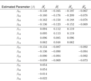
Consider the scenario of two binary variables defined asX1 = 0,1 and X2 = 0,1. We are

in-terested in whether independent variableX1 has a different effect on log time-conditional survival

probabilities depending on values ofX2. That is, we are interested in assessing whether there is

an interaction effect. Define k = 4strata by{X1, X2} ∈ {(0,0),(0,1),(1,0),(1,1)}and letp = 3,

indicating that for each strata there are three log time-conditional survival probability estimators.

Under this scenario, theKp-length vector of log time-conditional survival probabilities is given by

logCS= (logCS11,logCS12,logCS13, . . . ,logCS41,logCS42,logCS43)0.

We begin by defining the full saturated model given by

whereXf is a 12×12 design matrix andβf is a vector of length12×1. For the full model, the

design matrixXf is given by

Xf = 

       

I3×3 03×3 03×3 03×3

I3×3 I3×3 03×3 03×3

I3×3 03×3 I3×3 03×3

I3×3 I3×3 I3×3 I3×3 

       

, (2.13)

andβf is given by

βf = (β01, β02, β03, β11, β12, β13, β21, β22, β23, β31, β32, β33)0.

Then the expectation for a single log time-conditional survival probability is given by

E(logCSkp) =β0p+β1pI(X1= 1) +β2pI(X2= 1) +β3pI(X1= 1)I(X2= 1),

whereI(·)is the indicator function defining the value ofk= 1,2,3,4. At time pointp= 1,2,3for this example, the log time-conditional survival probability for each of the four strata as a function ofpis given by

E[logCS1p] = β0p E[logCS2p] = β0p +β1p E[logCS3p] = β0p +β2p E[logCS4p] = β0p +β1p +β2p +β3p

. (2.14)

Similarly, for the reduced main effects model, the12×9design matrixXris given by

Xr= 

       

I3×3 03×3 03×3

I3×3 I3×3 03×3

I3×3 03×3 I3×3

I3×3 I3×3 I3×3 

       

, (2.15)

and the9×1vector,βr, is given by