Thesis by
Alden Walker
In Partial Fulfillment of the Requirements for the Degree of
Doctor of Philosophy
California Institute of Technology Department of Mathematics
Caltech Pasadena CA, 91125
2012
Acknowledgements
Abstract
Contents
Acknowledgements iii
Abstract iv
1 Introduction 1
1.1 Introduction . . . 1
1.2 Brief background . . . 1
1.3 Outline and results . . . 2
2 Background 5 2.1 Stable commutator length . . . 5
2.2 Quasimorphisms . . . 7
2.3 Free groups . . . 11
2.4 Fatgraphs . . . 14
2.5 Surface realizations . . . 16
3 Isometric endomorphisms of free groups 20 3.1 Introduction . . . 20
3.2 Isometries and non-isometries of scl . . . 21
3.3 Random homomorphisms are usually isometries . . . 22
3.4 Random fatgraph labelings are usually extremal . . . 29
4 Cyclic orders and quasimorphisms 38 4.1 Cyclic orders and compatibility . . . 38
4.2 Realizations and immersions . . . 39
4.3 Examples and consequences . . . 41
4.4 Transfer . . . 46
4.5 Symplectic rotation number . . . 50
4.6 Ends . . . 50
5 Dynamics and endomorphisms 68
5.1 Traintracks . . . 68
5.2 Endomorphisms and HNN extensions . . . 70
5.3 Geometric endomorphisms . . . 74
5.4 Norm-realizing surfaces in geometric HNN extensions . . . 79
6 Scylla 81 6.1 Overview . . . 81
6.2 Improving the combinatorial structure inscallop . . . 82
6.3 Thescyllaalgorithm for free groups . . . 89
6.4 Generalizing to finite cyclic free factors . . . 89
6.5 The completescyllaalgorithm . . . 97
6.6 Complexity and comparison withscallop . . . 98
List of Figures
2.1 Folding a Stallings graph . . . 11
2.2 A histogram of scl values . . . 13
2.3 A histogram of scl values for many words of length 40 inF2. . . 13
2.4 Unit balls in the scl norm . . . 14
2.5 Fatgraphs . . . 14
2.6 A labeled fatgraph . . . 15
2.7 A basic fatgraph realization . . . 19
3.1 A histogram of sclF2(i∗∂Σ) for 7500 random surface realizations of an index 2 subgroup. 22 3.2 A local move to replace a partial match with a perfect match. . . 25
3.3 Diagram of inequalities for the proof of Proposition 3.3.4 . . . 26
3.4 The vertex quasimorphism construction on a thrice-punctured sphere. . . 30
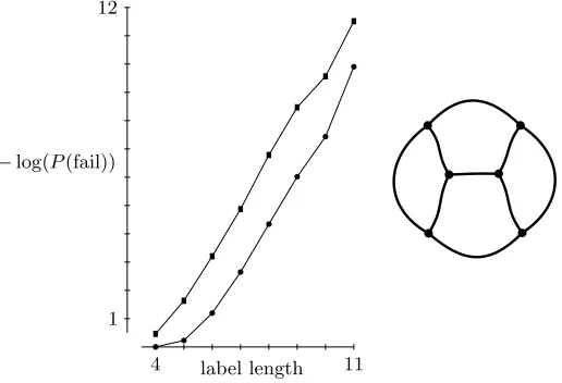
3.5 Experimental verification of the fatgraph labeling theorem . . . 36
3.6 Using homomorphisms to improve vertex quasimorphism success rate . . . 37
4.1 A cyclic order on words induced from a cyclic order on generators . . . 39
4.2 Comparing intrisic vs pullback cyclic orders . . . 40
4.3 Applying an automorphism and folding to produce an immersed fatgraph . . . 42
4.4 Blocked fatgraphs . . . 45
4.5 A picture of a vimersion . . . 49
4.6 Another picture of the same vimersion . . . 49
4.7 Taking the total preimage of a fatgraph . . . 55
4.8 Rewriting labels on a fatgraph . . . 55
4.9 Maximal trees in fatgraphs . . . 56
4.10 An extremal fatgraph forC=x2+y+yXY2X and a maximal tree. . . . 57
4.11 Mapping the Cayley graph ofF intoS1, and pictures of invariant triples of ends . . . 60
4.12 Invariant 4-tuples of ends, as described in Example 4.6.10. . . 61
4.13 Illustrating a fatgraph boundingC and the action ofF/Gn. . . 65
5.1 Appliying an endomorphism to a quadpod . . . 75
5.2 Possibilities when applying an endomorphism to a quadpod . . . 77
6.1 A fatgraph structure . . . 83
6.2 A rectangle . . . 83
6.3 A polygon and incident rectangles . . . 84
6.4 Cutting a polygon into pieces . . . 84
6.5 Central and intrface edges . . . 85
6.6 A group polygon . . . 90
6.7 Creating a group polygon . . . 92
6.8 Pinching to reduce the number of sides of a group polygon . . . 92
6.9 Cyclic fatgraph examples . . . 93
Chapter 1
Introduction
1.1
Introduction
In this chapter, we give a very brief introduction to the subjects of this thesis and state our main results. In Chapter 2, we give more detailed background material, and the subsequent chapters form the main body.
1.2
Brief background
1.2.1
Stable commutator length
LetGbe a group and letX =K(G,1). There are homology chain groupsC∗(G,Z) =C∗(X,Z), and
we denote 1-boundaries byB1(G,Z). The spaceB1(G,Z) is the free Zmodule spanned by formal
sumsPn
i=1gi of group elements with the property that there is a surface mapf :S→X whereS
hasnboundary components{(∂S)i}andf((∂S)i) =γias loops inX, andγi is a loop representing
the conjugacy class ofgi.
The study of stable commutator length is motivated by the question: given a collection of loops which bound a surface inX, what is the simplest surface that they bound? It is natural to stabilize the definition; that is, to allow sufaces to have multiple boundary components mapping to the same loop, and perhaps with degree greater than one. A surface map f :S →X is admissible for P
igi
if the following commutative diagram holds
S −−−−→f X
x
x
`n i=1γ
∂S −−−−→∂f `n
i=1S 1
i ,
where eachS1i is a copy ofS1 andγi:Si1→X represents (the conjugacy class of)gi. Furthermore, we definen(S, f) to be the integer such that∂f∗[∂S] =n(S, f)`iS
1
i
how many times the surface wraps around each loop. We define
scl(X
i
gi) = inf
(S,f)
−χ−(S) 2n(S, f),
where χ−(S) is the Euler charateristic disregarding disk and sphere components. It extends to
B1(G;R), and we defineB1H(G) =B1(G;R)/hxyx−1 =y, yn =nyi. This will be our main space of
study. We call an admissible surface mapextremal for a chain if it realizes the infimum.
Stable commutator length is mysterious and complicated, even in groups as simple as free groups.
1.2.2
Quasimorphisms
A functionφ:G→Ris ahomogeneous quasimorphismif there exists a finite real numberD(φ)<∞
such that|φ(x) +φ(y)−φ(xy)| ≤D(φ) for allx, y∈G, andφ(xn) =nφ(x) for allx∈Gandn∈Z.
We denote the space of homogeneous quasimorphisms byQ(G). Note thatQ(G) contains the space
H1(G) of real-valued homomorphisms ofG.
Homogeneous quasimorphisms extend by linearity to give well-defined functions on BH
1 (G).
These functions are intimately connected with scl.
Theorem (Bavard duality, Theorem 2.79 in [8], generalizing [2]). ForC∈BH
1 (G),
scl(C) = sup
φ∈Q(G)/H1(G)
φ(C) 2D(φ).
This theorem says that the normed vector space (Q(G)/H1(G), D(·)) is the functional dual space of the (pseudo-) normed vector space (B1H(G),scl). We call a quasimorphism extremal for a chain
inB1H(G) if it realizes the supremum.
WhenGis a free group, scl is a genuine norm onBH
1 (G).
1.3
Outline and results
The general theme of this thesis is that we can leverage the combinatorial structure of surface maps into free groups in combination with an understanding of the geometry of surfaces to prove results involving stable commutator length and quasimorphisms. In addition to theorems, we also give several interesting constructions, and the final chapter gives an algorithm. These tools allow us to gain a better understanding of the situation, and they promote further study.
Let G and H be groups. We say that a homomorphism φ : G → H is an isometry for scl if sclH(φ(C)) = sclG(C) for allC∈B1H(G). As we will see, this is a complicated condition, and it is
Let Fk andFl be free groups of rankk andl. We define a random homomorphism of length n φ : Fk → F` to be a homomorphism obtained by defining φ on the generators of Fk to be words
selected uniformly at random from the ball of radiusninF`. We show that
Theorem (3.3.11; Random isometry theorem). A random homomorphism ϕ: Fk → Fl of length
n between free groups of ranksk, l is an isometry ofscl with probability 1−O(C(k, l)−n) for some constant C(k, l)>1.
The random isometry theorem shows that an algebraically random map preserves scl. In free groups, it is natural to define a geometrically random surface map, and we show that these maps are extremal, which is the natural analog of isometric. For the purposes of this introduction, it suffices to know that afatgraphis essentially a combinatorial description of a surface map into a free group (Figure 2.6, for the impatient).
Theorem(3.4.11; Random fatgraph theorem). For any combinatorial fatgraphYˆ, ifY is a random fatgraph overFk obtained by labeling the edges ofYˆ by words of lengthn, thenS(Y)is extremal for
∂S(Y) and is certified by the extremal quasimorphism HY, with probability 1−O(C( ˆY , k)−n) for
some constant C( ˆY , k)>1.
Here HY is a quasimorphism constructed in a combinatorial way from the labeling on Y.
The previous theorems show that, in a certain sense, the generic picture of scl in free groups is well understood (in addition, see [14]). However, a detailed picture is very complicated. A realization of a free group as the fundamental group of a hyperbolic surface induces a naturalrotation quasimorphism via the circle action at infinity. Associated to such a rotation quasimorphism is ageometric face of the scl norm ball inBH
1 (F). These faces are important and interesting. In Chapter 4, we explore the
space of rotation quasimorphisms and geometric faces of the scl norm ball. We show some interesting structural properties of the set of geometric faces.
Theorem(4.3.8; Extremal rotations quasimorphisms). LetF2be a free group of rank2. There exist
infinitely many commutators for which the rotation quasimorphism from any surface realization is extremal. There exist infinitely many commutators for which there is no surface realization giving an extremal rotation quasimorphism.
A slightly less general statement is true for free groups of arbitrary rank.
Rotation quasimorphisms induced by surface realizations are very natural and have many nice properties. However, it is trivial to see that we must search for larger classes of quasimorphisms, for a rotation quasimorphism from a surface realization takes integer values. There are many chainsC∈
BH
1 (Fk) for which scl(C) is not in 12Z. Therefore, we cannot hope to find an extremal quasimorphism
In the transfer construction, we lift a quasimorphism from a finite index subgroup to the whole group. This provides a new class of quasimorphisms, and we show that this is nontrivial by exhibiting an infinite family of examples for which they are extremal.
Proposition (4.4.8). Let w(n) = x2+yn+yx−1yn+1x−2 ∈F
2=hx, yi. Then scl(w(n)) = 22nn+1+2,
and there is a family φn of transfers of rotation quasimorphisms from finite index subgroups of F2
such that φn is extremal forw(n).
In addition, we show that in certain cases, we can take limits of the transfer procedure to obtain limiting quasimorphisms, and we give examples of chains for which these limit transfers are extremal. Proposition (4.7.8). Let F2 be a free group of rank 2. There exist sequences φn of transfers of
rotation quasimorphisms on finite index subgroups of F2 with index n such thatφn converges to a
weak-* limitφ∞, and there are chains for whichφ∞ is extremal.
In Chapter 5, we study the dynamics of endomorphisms on free groups. We call an endomorphism
φ:Fk→Fk geometric if there is a realization of Fk as the fundamental group of a smooth surface Σ and an immersion ψ : Σ → Σ such that ψ∗ = φ. A geometric automorphism must be in the
mapping class group of a surface Σ withπ1(Σ)∼=Fk, and these elements are rather rare in Out(Fk).
In contrast, we show:
Theorem (5.3.6; Geometric endomorphisms). A random endomorphismφ:Fk →Fk of lengthnis
geometric with probability1−C(k)−n.
The theorem is proved by giving a simple combinatorial condition guaranteeing that an endo-morphism is geometric.
In combination with results about scl and quasimorphisms, this produces manyπ1-injective maps
of surface groups into HNN extensions of free groups and gives simple conditions certifying their injectivity.
In Chapter 6, we give an algorithm, scylla, to compute scl in free products of cyclic groups. Here the cyclic groups can be finite or infinite, so this generalizes thescallopalgorithm (on which
Chapter 2
Background
The content of this thesis comprises several results involving stable commutator length, quasimor-phisms, and surface maps. There is a significant amount of overlap in the background material required for the various chapters, so it is useful to collect it in one place. Therefore, in this chapter, we present a review of stable commutator length, quasimorphisms, and surface realizations of free groups.
2.1
Stable commutator length
2.1.1
Definition
LetG be a group and [G, G] the commutator subgroup of G. Ifg ∈[G, G], then g can be written as a product of commutators, and we define thecommutator length cl(g) to be the least number of commutators whose product isg.
Commutator length is complicated and difficult to understand, mostly because the set of com-mutators in a general group can contain elements which do not “look” like comcom-mutators. In fact, in a finite nonabelian simple group, every element is a commutator [27]! Changing the context from algebra to topology gives a more intuitive picture. The commutator length ofgis the least genus of a surface with one boundary component which maps into a K(G,1) in such a way that the image of its boundary loop maps to a loop representing the conjugacy class ofg.
Definition 2.1.1. Thestable commutator length scl(g) ofg is defined
scl(g) = lim
n→∞
cl(gn) n .
Let C = Pk
i=1gi be a formal sum of elements gi ∈ G. If [C] = 0 inH1(G;Z), in which case C ∈ B1(G;Z), the space of boundaries, then there exists a surface map S → K(G,1) with n
boundary components such that the images of the boundary components in π1(K(G,1)) =Gmap
to the conjugacy classes of thegi. We say that a surface mapf :S→K(G,1) isadmissible for the formal sumPn
i=1gi if the following commutative diagram holds:
S −−−−→f K(G,1)
x x `n i=1γ
∂S −−−−→∂f `n
i=1S 1
i ,
where each Si1 is a copy of S1 and γi : Si1 → K(G,1) represents (the conjugacy class of) gi. Furthermore, we definen(S, f) to be the integer such that ∂f∗[∂S] = n(S, f)`iS
1
i
. Informally, a surface map is admissible for a collection of loops if its boundary maps to some multiple of the loops. Note that an admissible surface map may have multiple boundary components mapping to the same copy ofS1, and in fact with different degrees.
Definition 2.1.2. Let the functionχ−(·) be the Euler characteristic disregarding disk and sphere components. Then define
scl k X i=1 gi ! = inf S,f
−χ−(S) 2n(S, f),
where the infimum is taken over all surface maps (S, f) which are admissible forPk
i=1gi.
Remark 2.1.3. Ifg ∈[G, G], theng∈B1(G;Z). It is a proposition that Definitions 2.1.1 and 2.1.2
agree for such elements ofB1(G;Z). See Propositions 2.10 and 2.74 in [8]. We have omitted a more
algebraic generalization of Definition 2.1.1 because we will not need it.
Because scl has nice linearity properties (Lemmas 2.75 and 2.76 in [8]), it extends by linearity toB1(G;Q). Furthermore, it is continuous, so it extends by continuity toB1(G;R). Henceforth, we
will supress the coefficient group in the notation and always take it to beR, so B1(G) =B1(G;R).
Definition 2.1.4. LetH(G) be the subspace ofB1(G) spanned by all elements of the formhgh−1−g
andgn−ng forg, h∈Gandn∈
Z. We defineB1H(G) =B1(G)/H(G).
Lemma 2.1.5(§2.6.1 in [8]). For any groupG,sclgives a well-defined function onBH1 (G); that is, sclvanishes onH(G).
It is more natural to work in B1H(G). We have the following properties of scl, from§2.6.1 in [8]:
Homogeneity. Forg∈Gandn >0, scl(gn) =nscl(g).
Sublinearity. Forx, y∈BH
1 ((G), scl(x+y)≤scl(x) + scl(y).
In other words, scl is always a pseudo-norm onBH
1 (G). It is not always a norm because it might
vanish on a nonzero element. However, if Gis word hyperbolic, or in particular free, then scl is a genuine norm [10].
2.1.2
Extremal surfaces and examples
Intuitively, scl(C) gives the most “efficient” surface which bounds loops representingC in K(G,1). It is not true in general that the infimum is actually realized by a surface map. For example, there are groups for which scl takes transcendental values on certain elements (see [33]). In particular, these values are not rational, so they cannot be realized by finite surface maps.
However, sometimes there is a surface map realizing the infimum. That is, for a chainC∈BH
1 (G),
a surface mapf :S →K(G,1) such that scl(C) =−χ−(S)/2n(S, f). We call such surfacesextremal forC.
Example 2.1.6. Let G be any group, and let [g, h] be a commutator. Then scl([g, h]) ≤ 1/2. To see this, observe, that [g, h] is the boundary of a tautological once-punctured torus in a K(G,1). Therefore, scl([g, h])≤ −(−1)/2 = 1/2.
Example 2.1.7. LetG=ha, bi. Thena+b+a−1b−1∈B1H(G), and scl(a+b+a−1b−1)≤1/2. To see this, observe that there is a simple thrice-punctured sphere with three boundary components mapping toa, b, anda−1b−1. Since a thrice-punctured sphere has Euler characteristic−1, we have scl(a+b+a−1b−1)≤ −(−1)/2. In fact, this surface is extremal.
Theorem 2.1.8 (§4.1 in [8]). For any chain C ∈BH
1 (F) forF a free group, an extremal surface
forC exists.
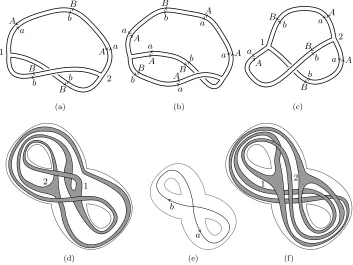
Figures 2.3, 2.4a, and 2.4b give some pictures of scl in free groups.
2.2
Quasimorphisms
2.2.1
Definition
LetGbe a group, and letφ:G→Rbe a map. If φ(g) +φ(h)−φ(gh) = 0 for all g, h∈G, thenh
is a homomorphism. We generalize this:
Definition 2.2.1. Letφ:G→R. If there exists a finiteD such that|φ(g) +φ(h)−φ(gh)| ≤D,
Let ˆQ(G) denote the real vector space of quasimorphisms onG. Ifφ∈Qˆ(G) satisfiesφ(g−1) =
−φ(g), then we callφantisymmetric. Theantisymmetrizationφ0is definedφ0(x) = 12(φ(x)−φ(x−1)).
Note that antisymmetrization does not increase defect. Ifφ(gn) =nφ(g) for alln∈
Z, then we call φhomogeneous. LetQ(G) denote the space of homogeneous quasimorphisms. Ifφ∈Qˆ(G), then we define the homogenization ¯φ:
¯
φ(g) = lim
n→∞ φ(gn)
n .
This limit exists, and the homogenization satisfies |φ(g)−φ¯(g)| ≤ D(φ), by Lemma 2.21 in [8]. Furthermore, D(φ) ≤ D( ¯φ) ≤ 2D(φ) by Corollary 2.59 in [8]. Notice that the space H1(G) of
homomorphisms onGsits inside the space of homogeneous quasimorphisms.
2.2.2
Duality with
scl
Homogeneous quasimorphisms extend by linearity to give well-defined functions onBH1 (G). These functions are intimately connected with scl.
Theorem 2.2.2 (Bavard duality, Theorem 2.79 in [8], generalizing [2]). ForC∈B1H(G),
scl(C) = sup
φ∈Q(G)/H1(G)
φ(C) 2D(φ).
This theorem says that the normed vector space (Q(G)/H1(G),2D(·)) is the functional dual space
of the (pseudo-) normed vector space (BH
1 (G),scl). If a quasimorphism realizes the supremum, then
we call itextremal forC. By the Hahn-Banach theorem, an extremal quasimorphism forC always exists. This is in contrast to extremal surfaces forC, which might not exist.
Observe that if φ ∈ Q(G) is any quasimorphism, and f : S → K(G,1) is any surface map admissible forC, then
φ(C)
2D(φ) ≤scl(C)≤
−χ−(S) 2n(S, f).
The most satisfying way to compute scl, then, is to exhibit a surface map and a homogeneous quasimorphism which gave matching upper and lower bounds.
2.2.3
Counting quasimorphisms
In free groups, there is a very natural class of quasimorphisms: those that count subwords.
Definition 2.2.3. Let σ and w be words in a free group F. Define Cσ0(w) to be the number of
(possibly overlapping) occurrences ofσas a subword ofw. Define thecounting function Cσ to be
Cσ(w) = lim
n→∞
Cσ0(wn)
Thebig counting quasimorphismHσ is then
Hσ(w) =Cσ(w)−Cσ−1(w).
Big counting quasimorphisms are easy to compute. Let w denote the cyclic, and cyclically reduced, word obtained fromwby writingw around a circle and deleting any cancelling subwords at the beginning and end ofw.
Lemma 2.2.4. Cσ(w) =Cσ0(w).
Proof. Any subword ofwn is a cyclic subword ofw.
We can also count disjoint subwords:
Definition 2.2.5. Let c0σ(w) count the maximum number of disjoint copies ofσ as a subword of
w. As above, we definec0σ(w) = limn→∞c0σ(wn)/n. Thesmall counting quasimorphism hσ is
hσ(w) =cσ(w)−cσ−1(w).
Both the big and small counting quasimorphisms are, as advertised, quasimorphisms, and they are homogeneous. They were introduced by Brooks in [5] and generalized to hyperbolic groups by Epstein-Fujiwara [19] and Fujiwara [20]. Also see [10].
Big counting quasimorphisms are easier to compute, but small counting quasimorphisms have a uniformly bounded defect.
Lemma 2.2.6 (Corollary of Proposition 2.30, [8]). For any small counting quasimorphism hσ, we haveD(hσ)≤6.
Note that there is a difference in notation in [8]; our counting quasimorphisms are already homogenized.
Brooks counting quasimorphisms are simple linear combinations of counting functions. One might wonder whether any other linear combinations yield quasimorphisms. The answer is no. Lemma 2.2.7. If S is a finite set of words, and P
σ∈SCσ is a homogeneous quasimorphism, then
P
σ∈SCσ= 12Pσ∈SHσ. The analogous statement is true for small counting quasimorphisms.
Proof. SinceP
σ∈SCσ is a homogeneous quasimorphism, it is its own antisymmetrization. But its
antisymmetrization is exactly the linear combination of Brooks counting quasimorphisms above.
2.2.4
Rotation quasimorphisms
There is a universal central extension
0→Z→Homeo+(S1)∼→Homeo+(S1)→0.
The group Homeo+(S1)∼ can be thought of as the group of orientation preserving homeomorphisms
of Rwhich commute with integer translation, or equivalently, the group of homeomorphisms of R
which cover homeomorphisms ofS1.
There are a few different ways to define the rotation number on Homeo(S1) and Homeo+(S1)∼. We define rot∼: Homeo+(S1)∼→Rby
rot∼(f) = lim
n→∞ f◦n(0)
n .
This limit is well defined, and any other point can take the place of 0; the resulting limit is the same. This map descends to rot : Homeo+(S1) →
R/Z, which is Poincar´e’s rotation number. If
we let t ∈ Homeo+(S1)∼ be the generator of the center, so t is integer translation by 1, then we
observe that rot(t◦n◦f) =n+ rot(f). The function rot∼ : Homeo+
(S1)∼ →
R is a homogeneous
quasimorphism with defect 1.
For any action of a group on a circle ρ : G → Homeo+(S1), there is an associated bounded Euler class eb(ρ,Z) ∈ Hb2(G;Z). The image e(ρ;Z) in H
2(G;
Z) is the ordinary Euler class. The
representation lifts toρ∼:G→Homeo+(S1)∼if and only if the ordinary Euler classe(ρ,
Z) vanishes.
If the representation does lift, then the different lifts are parameterized byH1(G,
Z) (essentially, by
choosing a particular lift for each generator).
The Euler class determines the representation up to semiconjugacy:
Theorem 2.2.8 (Ghys [21]). Two actionsρ1, ρ2:G→Homeo(S1)give rise to the sameeb(ρ;Z)∈ H2
b(G;Z)if and only if ρ1 and ρ2 are semiconjugate; i.e., if and only if there is some third action
ρand monotone mapsπ1, π2:S1→S1 such thatρiπi=πiρfori= 1,2.
For background on the Euler class and rotation number, see [6], [31], and [22].
We will be interested in the pullback of the rotation quasimorphism via representations, and we therefore need to know how the defect behaves under pullback.
Proposition 2.2.9 (Thurston [31], Proposition 3.3). Let ρ:G→Homeo+(S1)be a representation
with associated rot∼. Then either ρ is semiconjugate to a group of rigid rotations, in which case
D(rot∼) = 0, or else ρis semiconjugate to a minimal action with centralizer of finite order n, and
2.3
Free groups
2.3.1
Notation
We let Fk be a free group of rank k. Usually, our free groups will be generated bya, b, . . ., and sometimes by a1, . . . , ak. Where convenient, we will denote the inverses of generators by capital
letters, soA=a−1. We let Xk be aK(Fk,1). For simplicity, we will always takeXk to be a rose.
That is,Xk is a simplicial complex with a single 0-cell and k1-cells, each thought of as a directed edge labeled by a generator ofFk.
2.3.2
Stallings graphs
It is very convenient to think of free groups and subgroups of free groups as the fundamental groups of graphs.
Definition 2.3.1. A Stallings graph [30] G over a free group Fk is a directed graph with edges
labeled by generatorsa1, . . . , ak ofFk.
A directed loop in G gives a word inFk by reading edge labels in order as appropriate (going across an edge with the opposite orientation reads off the inverse of the generator). Therefore, a Stallings graph overFk has a natural identification with a subgroup ofFk. Every subgroupH ofFk
has an associated Stallings graph: for example, take a set of generators forH, and take the Stallings graph which is the rose on a set of loops, each labeled with a generator ofH.
a
a a
b
a
a b
Figure 2.1: A Stallings graph overha, biwith fundamental group the subgrouphaa, abi. Folding the two middle edges together produces a folded Stallings graph for the same subgroup (right).
A vertex v of a Stallings graph is folded if there is at most one incident incoming edge with any label and at most one incident outgoing edge with any label. A Stallings graph is folded if each of its vertices is folded. If a Stallings graph contains a vertex which is not folded, orunfolded, then we can perform a local transformation of the Stallings graph which folds the offending edges together. If there are two edges with the same label and same origin and destination, then we simply remove one of them — we think of it as folding the edges together. If there are two incoming (resp outgoing) edges e1 and e2 with the same direction and label, then we identify together the origin
(resp destination) vertices of e1 and e2 and remove one ofe1 and e2. Repeatedly performing the
operation does not change the subgroup ofFk associated with the Stallings graph. Therefore, every
subgroup ofFk is associated with a folded Stallings graph. See Figure 2.1.
2.3.3
Subgroups and covers
One of the strengths of using Stallings graphs to understand subgroups ofFk is that the finite index subgroups ofFk are exactly the labeled covers of the Stallings graphXk. For example, this provides a simple proof of the following.
Lemma 2.3.2. Given a finitely generated proper subgroup H (Fk, there is a finite index proper
subgroupN (Fk so that H ⊆N.
Proof. Take a Stallings graph forH and fold it. IfH is a proper subgroup, the resulting graph will not be a K(Fk,1). The only reason it is not a cover is that it is missing some edges. Add edges
(and a vertex, if necessary) so that (1) there is more than one vertex and (2) every vertex has an incoming and outgoing edge labeled with each generator. The result is a finite cover of Xk whose
fundamental group is therefore a finite index subgroupN containingH.
Of course, this is also consequence of the more powerful (and harder to prove) fact that finitely generated subgroups of a free group are separable (free groups are LERF) (see [23]).
2.3.4
The
scl
norm ball
In a free groupFk, scl is a norm onB1H(Fk) (see [10]). It is natural to wonder what the scl norm ball
looks like, since this is a generalization of wondering what the scl spectrum looks like. In fact, the scl norm ball in a free group is an infinite dimensional polyhedron, in the sense that its intersection with any finite-dimensional subspace ofBH
1 (Fk) is a polyhedron. This is a consequence of Calegari’s
scallopalgorithm to compute scl in free groups; see [7],§4.1.
While they are polyhedra, these finite-dimensional slices of the norm ball can be quite compli-cated. In the large scale, however, scl looks like an L1 norm; see [14].
2.3.5
Pictures of
scl
in free groups
It is motivating to observe the complexity of scl through experiments. Pictures of scl tend to be simple at a large scale and complex at a small scale, and this is formalized in [11] and [14].
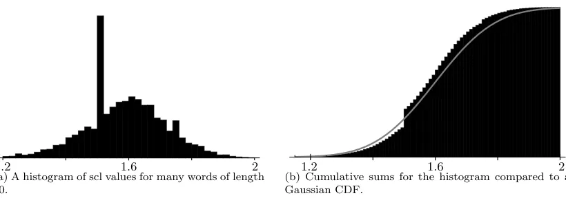
Figure 2.2a show a histogram of the scl values of many random words of length 40 inF2. Observe
1.2 1.6 2
(a) A histogram of scl values for many words of length 40.
1.2 1.6 2
(b) Cumulative sums for the histogram compared to a Gaussian CDF.
Figure 2.2: Comparing a histogram of scl values to its cumulative distribution function.
We also remark that experimental data can be misleading: [14] proves a convergence result which occurs so slowly that we cannot hope to observe it with our current experimental capabilities.
Compare Figures 2.2a and 2.2b to a histogram of the same data with very small bins, as shown in Figure 2.3. Note the obvious complexity and self-similarily. This is discussed in more detail in [9]. See also [13].
1.4 1.5 1.6 1.7 1.8
Figure 2.3: A histogram of scl values for many words of length 40 inF2. Some of the vertical bars
are not to scale.
Figure 2.4a shows the scl unit ball in the 2-dimensional subspace of BH
1 (F2) spanned by the
chainsABabbAbaBB andAABBabbb+Ba. For example, the starred vertex of the polygon, which is located at (6/5,4/5), indicates that
scl(6ABabbAbaBB+ 4AABBabbb+ 4Ba) = 5.
Even with these relatively short chains, there is evident complexity in the unit ball. Figure 2.4b shows the unit ball in the 2-dimensional subspace spanned by baaaaaBBABBBAAbAbbAb and
1
1 ∗
C1
C2
(a) The unit ball in the subspace spanned by the chainsC1=ABabbAbaBBandC2=AABBabbb+
Ba.
1 1
C1
C2
(b) The unit ball in a subspace spanned by two random word of length 20.
Figure 2.4: Unit balls in the scl norm.
2.4
Fatgraphs
2.4.1
Fatgraphs
Definition 2.4.1. Afatgraph, also known as a ribbon graph, is a graph with a specified cyclic order on the edges at each vertex.
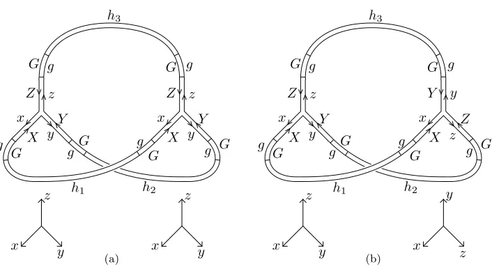
Figure 2.5: Two fatgraphs differing only in their cyclic orders, and their fattenings to a once-punctured torus and a trice-once-punctured sphere.
They are so called because a fatgraphY can be “fattened” to a surface, which we will denote by
S(Y); the cyclic order at each vertex ensures that the surface obtained is well-defined. See Figure 2.5. Definition 2.4.2. A fatgraphoverFk, or alabeled fatgraph, is a fatgraph with its edges labeled on
both sides by generators ofFk, subject to the condition that if an edge has the labelwon one side,
then the other side of the edge is labeled byw−1.
A labeled fatgraphY determines in a surface map fromS(Y) toXk: map each edge according to
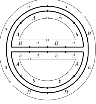
B b
a A B
b A
a
B
b
Figure 2.6: A labeled fatgraph; the induced surface map takes the boundary to the conjugacy class of the commutator [abAB, BaBA] =abABBaBAbb.
Conversely,
Lemma 2.4.3 ([18], Theorem 1.4). Let S be a surface with boundary, and let g : S → Xk be an
incompressible map. Then g is carried by a labeled fatgraph map. That is, there exists a labeled fatgraphY overFk so that g=i◦h, whereh:S→S(Y)is a homeomorphism, and i:S(Y)→Xk
is the map induced by the labeling ofY.
Since it is the heart of many of our computational arguments, we record the following corollary of Lemma 2.4.3 as another lemma.
Lemma 2.4.4. Let C ∈ B1H(Fk) be a chain, and let f : S → Xk be an admissible map. Then
there is a labeled fatgraphY with induced surface mapi:S(Y)→Xk such that −χ(S(Y))≤S and i∗(∂S(Y)) =f∗(∂S).
In other words, after possible compressions and homotopy, any admissible map is carried by a labeled fatgraph.
2.4.2
Stallings fatgraphs
Recall that a Stallings graph is folded if there is at most one outgoing edge and one incoming edge labeled by a generator at each vertex. We define a labeled fatgraph to be folded if its boundary words are reduced. Note that this is equivalent to saying that for every vertex, there are no cyclically adjacent edges with the same direction and label. Here adjacent is well-defined because of the cyclic order.
It is not the case that we may obtain a folded labeled fatgraph from an unfolded one by folding. The process of doing local folds can result in losing the fatgraph structure.
2.5
Surface realizations
2.5.1
Surface realizations
Definition 2.5.1. A surface realization of a free groupFk is a pair (Σ, f), where Σ is a smooth surface with boundary, andf is a homotopy equivalencef :Xk →Σ.
We consider the set of surface realization modulo the following equivalence relation. Two surface realizations (Σ1, f1) and (Σ2, f2) are equivalent if there is a diffeomorphismφ: Σ1 →Σ2 such that
φ◦f1 is homotopic tof2.
Because we have identifiedFk∼=π1(Xk), a surface realization induces an isomorphismf∗:Fk→ π1(Σ) up to inner automorphisms of Fk.
Definition 2.5.2. A hyperbolic surface realization ofFk is a pair (Σ, f), where Σ is a hyperbolic
surface with geodesic boundary, andf :Xk →Σ is a homotopy equivalence. Two hyperbolic surface
realizations (Σ1, f1) and (Σ2, f2) are equivalent if there is an isometryφ: Σ1→Σ2 such thatφ◦f1
is homotopic tof2.
Definition 2.5.3 (Alternate definition). A hyperbolic surface realization of Fk is a discrete faith-ful representation ρ : Fk → PSL(2,R). Two hyperbolic surface realizations are equivalent if the
representations are conjugate. In the above notation, we let (Σρ, fρ) denote the hyperbolic surface realization given byρ.
Given a hyperbolic surface realization, we can forget the hyperbolic structure to obtain a surface realization. We can therefore think of the set of surface realizations as π0 of the space of
hyper-bolic surface realizations. Conversely, a surface realization can be stiffened to a hyperhyper-bolic surface realization by choosing a hyperbolic structure on Σ.
Given a free groupFk, there is a finite set of topological types of surfaces Σ with boundary such that π1(Σ) ∼= Fk. Therefore, the space of hyperbolic surface realizations decomposes as a union
of Teichm¨uller spaces, with one component for each topological type of surface Σ and (because we mod out by the equivalence relation above) coset of the mapping class group of Σ in the outer automorphisms Out(Fk).
2.5.2
Rotation quasimorphisms from realizations
The action of PSL(2,R) on H2 induces an action on the ideal boundary∂
H2=S1 by
homeomor-phisms, giving rise to an inclusion PSL(2,R)→Homeo+(S1).
Any representation ρ : Fk → PSL(2,R) → Homeo+(S1) lifts to ρ∼ : Fk → Homeo+(S1)∼
becauseH2(F
k;Z) = 0. We denote by rotρthe associated class of rot∼inQ(Fk)/H1(Fk). Note that
Ifρis a discrete, faithful representation associated with a hyperbolic surface realization, the quasi-morphism rotρtakes integer values. Because rot is a continuous function (on the space Homeo+(S1))
and the Teichm¨uller component containingρis connected, it follows that rotρ is constant over the
entire component. In other words,
Lemma 2.5.4. LetΣρ1 andΣρ2 be two hyperbolic surface realizations in the same component. Then rotρ1 = rotρ2.
If (Σ, f) is a surface realization ofF, we will denote the associated rotation quasimorphism by rot(Σ,f), or just rotΣ iff is understood.
If (Σ, f) is a hyperbolic surface realization, each Γ in B1 has a canonical representative Γ :
`
iS
1
i →Σ (at least up to reparameterization), namely the geodesic representative. We say that Γ
virtually bounds an immersed surfaceif there is some immersion g:S→Σ which is admissible for a geodesic representative Γ. This is equivalent to saying that we can find a hyperbolic structure on
S with geodesic boundary for whichg:S→Σ is a local isometry.
The following theorem indicates a deep relationship between the geometry and combinatorics of
B1H(Fk) and the set of surface realizations ofFk.
Theorem 2.5.5 (Calegari [7], Theorems A and B). Let (Σ, f) be a surface realization of Fk, and let∂Σ∈B1H(Fk)be the associated chain.
1. There is a codimension1faceπΣof the unit ball of thesclnorm, and the chain∂Σprojectively
intersects its interior.
2. A chainΓprojectively intersectsπΣif and only if, for any hyperbolic surface realization
stiffen-ing(Σ, f), the geodesic representative ofΓvirtually bounds an immersed surface. Additionally, a surface admissible forΓis extremal forΓif and only if it is homotopic to an immersion with geodesic boundary.
3. rotΣ is the unique (class of ) quasimorphism inQ(Fk)/H1(Fk)with defect1 which is extremal
for elements projectively intersecting the interior of πΣ.
Theorem 2.5.5 implies the following ridigity result for the interaction of extremal surfaces and extremal quasimorphisms, valid for any group:
Corollary 2.5.6. Let G be any group. Let C ∈BH
1 (G), and let f :S → K(G,1) be an extremal
surface forC. Then any quasimorphismφ∈Q(G)with defect1 which is extremal forC restricts to the tautological representationrotS onπ1(S), up to an element ofH1(S;R).
extremal for∂S. Note thatD(f∗φ) = 1, certified by its value on∂S. By Theorem 2.5.5, this implies thatf∗φ= rotS up to an element ofH1(S;R).
In the preceeding corollary, it is important to note that the pullback of any extremal quasimor-phism to any extremal surface gives the rotation number up to an element ofH1(S;
R),notH1(S;Z)
orH1(G;
R). This is a source of potential confusion.
A surface realization induces the rotation quasimorphism rotΣ, and Theorem 2.5.5 shows that
there is a strong relationship between geometry and the scl norm ball. The theorem associates a codimension one face of the scl norm ball with a surface realization.
Definition 2.5.7. We will call these codimension one facesgeometric faces of the scl norm ball.
2.5.3
Cyclic orders and basic surface realizations
Definition 2.5.8. Acyclic order on a setS is a choice of total ordering<p onS\pfor eachp∈S,
subject to the condition that ifp, q∈S, then the total orders<pand<q differ by a cut. That is, if x <py, thenx <qy unlessx <pq <py, in which casey <q x.
The intuition for a cyclic order is, naturally, that a cyclic order on a setS arranges the elements ofS cyclically, so while we cannot say if x < y, we can say whether any triple (x, y, z) is clockwise or counterclockwise. We will call a triple which is a counterclockwisepositive. It is sometimes useful to think of a cyclic order as a mapO:S3→ {−1,0,+1}which assigns±1 or 0 to a triple depending on whether it is counterclockwise, clockwise, or degenerate.
We will denote explicit cyclic orders by square brackets, so [x, y, z, w] gives a cyclic order on the set{x, y, z, w}. It is the same cyclic order as, for example, [y, z, w, x], but not the same as [x, y, w, z]. Cyclic orders and fatgraphs give a simple combinatorial way to describe surface realizations. Let
S ={a1, a−11, . . . , ak, a
−1
k } be a set of semigroup generators for Fk. Given a cyclic order O on S,
build a labeled fatgraph overFk as follows. First create a single vertexv. Then attach 2khalf-edges to v in such a way that the outgoing labels on each half-edge are arranged according to the cyclic orderOonS. Then glue the unattached ends of the half edges together, producing a fatgraph with a single vertex andkedges. Call this labeled fatgraph ΣO. There is a tautological mapfO :Xk →ΣO
obtained from following the labels.
Definition 2.5.9. The surface realization (fO,ΣO) as constructed above is thebasic fatgraph
real-ization induced byO.
a b
c
Xk
fO
ΣO
a A
b B
c C
Figure 2.7: The basic fatgraph realization ofF3=ha, b, ciinduced by the cyclic order [a, b, A, B, c, C].
The surface ΣO has two boundary components, given by the conjugacy classes of the wordsC and aBAbc.
2.5.4
A formula for rotation number
For a basic fatgraph realization, there is a simple combinatorial formula for the associated rotation number rotΣO, which for simplicity we will denote by rotO. The formula is given by Theorem 4.76
in [8].
If S is a set with a cyclic order O, and x, y, z ∈ S, we define the distance between x and y
avoiding z to be the number dz(x, y) such that xand y have dz(x, y)−1 elements between them
when arranged according to the total order<z onS. Then thetranslationfromxtoy avoidingzis
tz(x, y) =
dz(x, y) ifx <zy
−dz(x, y) ify <zx .
Theorem 2.5.10 (Theorem 4.76 in [8]).
rotO=
1 |S|
X
x6=y±1
ty−1(x, y)Cyx
While the formula may seem slightly arbitrary, this theorem is completely intuitive given the discussion in [8],§4.2.
Remark 2.5.11 (Important technical note). Theorem 2.5.10 gives the rotation quasimorphism in-duced by a cyclic order as a sum of counting functions. There is a difference in convention here which results in possible confusion: counting functions read subwords of the input word from left to right, but the circle action at infinity by Fk coming from the PSL(2,R) representation is a left
Chapter 3
Isometric endomorphisms of free
groups
3.1
Introduction
Definition 3.1.1. Given a homomorphismφ:G→H between groups, we say thatφis anisometry for scl if sclH(φ(C)) = sclG(C) for all C∈B1H(G).
It is natural to ask what conditions are sufficient to show that a homomorphism is an isometry. In this chapter, we show that a random homomorphism between free groups is an isometry, and we show that a random map of a fatgraph into a free group is extremal for its boundary. This chapter contains essentially the same material as [17].
More specifically, we prove
Theorem (3.3.11; Random isometry theorem). A random homomorphism ϕ: Fk → Fl of length
n between free groups of ranksk, l is an isometry ofscl with probability 1−O(C(k, l)−n) for some
constant C(k, l)>1.
By this theorem, the scl unit ball of a given free group is the same as infinitely many different subballs of itself.
We also prove
Theorem(3.4.11; Random fatgraph theorem). For any combinatorial fatgraphYˆ, ifY is a random fatgraph overFk obtained by labeling the edges ofYˆ by words of lengthn, thenS(Y)is extremal for ∂S(Y) and is certified by the extremal quasimorphism HY, with probability 1−O(C( ˆY , k)−n) for
some constant C( ˆY , k)>1.
3.2
Isometries and non-isometries of
scl
Let φ : G → H be a homomorphism between groups. Then since the image of a commutator is a commutator, sclH(φ(C)) ≤ sclG(C) for any C ∈ B1H(G). This inequality also holds for the
commutator length of any element g ∈ [G, G]: we have cl(φ(g)) ≤ cl(g). A natural question is whether a homomorphism is an isometry for scl; that is, whether sclG(φ(C)) = sclF(C) for all C ∈ BH1 (G). Analogously, we might ask if a homomorphism preserves commutator length. The
latter implies the former, but not the other way around. Example 3.2.1. An automorphism is an isometry.
Let us now specialize to free groups. A necessary condition for a homomorphism to be an isometry is that it is injective. However, this is not sufficient, as the following examples show.
Example 3.2.2. Let H be a genus 3 handlebody with boundary S = ∂S. Decompose S into two surfacesS1 andS2 of genus 1 and 2, respectively, separated by a curveγ=∂S1=∂S2. Denote the
inclusioni:S2→S.
Let T be the subcomplex of the complex of curves in S containing all the curves which bound disks in H. By [24], Theorem 2.7, there is a pseudo-Anosov homeomorphism φ of the boundary
∂S such thatd(φ(γ), T)≥2. Sinceφ(γ) is disjoint (i.e., distance 1 in the curve complex) from all the curves in φ(S2) representing elements of π1(S2), this implies that (φ◦i)∗ : π1(S2) → π1(H)
is injective. Now sclπ1(S2)(∂S2) = 1, since a surface is extremal in its own surface group for its boundary component. However, by construction, ∂(φ(S2)) = φ(γ) = ∂(φ(S1)), so φ(γ) bounds a
torus, so sclπ1(H)(∂φ(S2))≤1/2. Therefore, while (φ◦i)∗is injective, it is not an scl-isometry. In fact, this construction gives an example of an injective map of free groups that does not preserve commutator length. This gives a negative answer to a question of Bardakov [1], who asked whether an injection of free groups must preserve commutator length.
Example 3.2.3 (Nongeometric covers). Let H ⊆ Fk be a subgroup of finite index. If (Σ, f) is a surface realization of Fk, then there is a coverp: (Σ0, f0)→(Σ, f0) so that (Σ0, f0) is a realization of H. We call this a geometric cover. However, it is not the case that every surface realization of
H arises in this way. If (Σ, f) is a realization ofH which does not cover a realization ofFk, then we say that this is anongeometric cover. The inclusion mapp:H →Fk is injective, but we claim that sclFk(∂Σ) <sclH(∂Σ) for any nongeometric cover Σ realizing H. Thus the inclusion map of
any finite index subgroup is not an scl-isometry.
The proof of the claim relies on background developed more fully in [8], §4.2, but the essential ingredient is Theorem 2.5.5, and we give a sketch. If Σ is a nongeometric cover, then the conjugation action ofFk/H onH contains elements of Out(H) which are not in the mapping class group of Σ.
face (projectively). Therefore,
sclH(∂Σ +φ∂Σ)<sclH(∂Σ) + sclF(φ∂Σ).
Now we can compute sclFk(∂Σ) using the formula from Corollary 2.81 in [8]. This formula, together
with the above strict inequality, implies that sclFk(∂Σ)<sclH(∂Σ).
This holds for any nongeometric cover, so for any finite index subgroup, there are infinitely many elements ofB1H(H) whose scl strictly decreases under the (injective) inclusion map.
1 2
3 4
5
6 1
Figure 3.1: A histogram of sclF2(i∗∂Σ) for 7500 random surface realizations of an index 2 subgroup.
Figure 3.1 shows a histogram of scl(i∗∂Σ) for many realizations Σ of an index 2 subgroupG⊆F2,
where Σ is a four-punctured sphere. For all these realizations, we have sclG(∂Σ) = 1, but under the
inclusion mapi:G→F2 the scl must strictly decrease for nongeometric covers. The large spike at
1 is all the geometric covers.
3.3
Random homomorphisms are usually isometries
3.3.1
Bounds on
scl
LetFk be freely generated byx1, . . . , xk; if Γ∈B1H(Fk), we denote by|Γ|i the number of times that xiand x−i1 appear in Γ.
Proposition 3.3.1. With notation as above, we have an inequality
scl(Γ)≤ |Γ| −maxi|Γ|i 4 for any Γ∈BH
1 (Fk).
for Γ, we may assume it has a fatgraph structure by Lemma 2.4.4. Now cut out all rectangles corresponding to matched pairs ofx1 andx−11. Note that this actually means cutting out at most
|Γ|1/2 thrice-punctured spheres, What is left is an immersed subsurface S0 of S, and because we
cut out thrice-punctured spheres, −χ(S) ≤ −χ(S0) +|Γ|i/2. An essential immersed subsurface of an extremal surface is also extremal, by [7] (essentially, Theorem 2.5.5). Consequently S0 is extremal for its boundary Γ0, which lies in B1H(hx2, . . . , xni). We therefore have the inequality
scl(Γ)≤scl(Γ0) +|Γ|1/4. Repeating this argumentn−1 times yields
scl(Γ)≤scl(Γ00) +|Γ|1/4 +· · ·+|Γ|n−1/4
where scl(Γ00) = 0, since Γ00∈BH
1 (hxni). The proof follows.
Example 3.3.2. The bound in Proposition 3.3.1 is sharp, which we show by a family of examples. We first recall the free product formula ([8],§2.7), which says that ifG1 andG2 are arbitrary groups,
andgi∈G0i have infinite order, then sclG1∗G2(g1g2) = sclG1(g1) + sclG2(g2) + 1/2. Now, letFk be freely generated byx1, . . . , xk as above, and define
wk = [x1, x2][x3, x4]· · ·[xk−1, xk]
ifkis even, and
wk= [x1, x2][x3, x4]· · ·[xk−4, xk−3]xk−2xk−1xkx−k−11xkx
−1
k−2x
−2
k
ifkis odd.
For each i, we have scl([xi, xi+1]) = 1/2. Moreover, usingscallop([15]) one can check that
scl(xk−2xk−1xkx−k−11xkx−k−12x
−2
k ) = 1.
The free product formula then shows that scl(wk) = (k−1)/2, so Proposition 3.3.1 is sharp for all
k.
3.3.2
A small cancellation condition
Definition 3.3.3. LetAbe a set, and letF(A) be the free group onA. LetU be a subset ofF(A) withU∩U−1=∅, and letS denote the setU∪U−1. We say thatU satisfies condition (SA) if the
following is true:
(SA2) ifx, y∈S andy is not equal toxorx−1, then any common subwordsofxandy has length
strictly less than|x|/12; and
(SA3) ifx∈S and a subwordsappears in at least two different positions inx(possibly overlapping) then the length of sis strictly less than|x|/12.
LetB be a set, andϕ:B→U a bijection. Extendϕto a homomorphism ϕ:F(B)→F(A). We sayϕsatisfies condition (SA) ifU satisfies condition (SA).
Note that except for condition (SA1), this is the small cancellation condition C0(1/12). We will show the following:
Proposition 3.3.4. Let ϕ:F(B)→F(A) be a homomorphism satisfying condition (SA). Thenϕ
is an isometry ofscl.
Condition (SA1) forϕmeans that ifgis a cyclically reduced word inF(B), then the word inF(A) obtained by replacing each letter ofgby its image underϕis also cyclically reduced. This condition is quite restrictive — in particular it implies that|A| ≥ |B|, and even under these conditions it is not “generic” — but we will show how to dispense with it in§3.3.3. However, its inclusion simplifies the arguments in this section.
Example 3.3.5. The set{aa, bb} satisfies (SA1). The set{ab, ba}satisfies (SA1).
Supposeϕ:F(B)→F(A) satisfies condition (SA), and letY be a fatgraph with∂S(Y) in the image of ϕ, i.e., such that ∂S(Y) is a collection of cyclically reduced words of the form ϕ(g). By condition (SA1), eachϕ(g) is obtained by concatenating words of the formϕ(x±) forx∈B. We call these subwordssegmentsof∂S(Y), as distinct from the decomposition intoarcsassociated with the fatgraph structure. An arc is a pair of subwords of∂S(Y) which are glued together in the fatgraph structure.
Definition 3.3.6. Aperfect matchinY is a pair of segmentsϕ(x), ϕ(x−1) contained in a pair of arcs of∂S(Y) that are matched by the pairing. Apartial matchin Y is a pair of segmentsϕ(x), ϕ(x−1) containing subsegments s, s−1 in “corresponding” locations in ϕ(x) and ϕ(x−1) that are matched by the pairing.
The existence of a perfect match will let us replaceY with a “simpler” fatgraph. This is the key to an inductive proof of Proposition 3.3.4. The next lemma shows how to modify a fatgraphY to promote a partial match to a perfect match.
x X
x X
X x
x X
slide
−−−→
Figure 3.2: A local move to replace a partial match with a perfect match.
Proof. The fatgraphY can be modified by a certain local move, illustrated in Figure 3.2.
This move increases the length of the paired subsegments by 1. Perform the move repeatedly to obtain a perfect match.
Each vertex v of Y of valence |v|contributes (|v| −2)/2 to −χ(Y), in the sense that−χ(Y) =
P
v(|v| −2)/2. Since each vertexv ofY is in the image of|v|vertices in∂S, we assign a weight of
(|v| −2)/2|v|to each vertex of ∂S.
Lemma 3.3.8. Let Y be a fatgraph with ∂S(Y) =ϕ(Γ) and suppose that ϕ satisfies (SA). Then either Y contains a partial match, or−χ(Y)>|Γ|.
Proof. Observe that∂S(Y) decomposes into|Γ|segments, corresponding to the letters of Γ. Suppose
Y does not contain a partial match. Then since each vertex contributes (|v| −2)/2|v| to−χ(Y), it suffices to show that each segment of∂Y contains at least six vertices in its interior.
Suppose not. Then some segmentϕ(x) of∂Y contains a subsegmentsof length at least|ϕ(x)|/6 that does not contain a vertex in its interior. Either s contains a possibly smaller subsegment s0
which is paired with some entire segmentϕ(y), or at least half ofsis paired with some s−1in some
ϕ(y). In either case, since s is not a partial match by hypothesis, we contradict either (SA2) or (SA3).
Thus each segment contributes at least 7×((3−2)/2·3) = 7/6 to−χ(Y), and the lemma is proved.
We now give the proof of Proposition 3.3.4.
Proof of Proposition 3.3.4. Supposeϕ:F(B)→F(A) satisfies (SA) but is not isometric.
LetY be a fatgraph with∂S(Y) =ϕ(Γ) so that scl(ϕ(Γ))≤ −χ(S(Y))/2<scl(Γ) (the existence of such a Y follows from Lemma 2.4.3; for instance, we could take Y to be extremal). We will construct a new Y0 with ∂S(Y0) = ϕ(Γ0) satisfying scl(ϕ(Γ0))≤ −χ(S(Y0))/2 <scl(Γ0), and such thatY0 is shorter thanY. By induction on the size ofY we will obtain a contradiction.
cobounds a rectangle inS =S(Y) that can be cut out, replacingS with a “simpler” surfaceS0 for which∂S0is also in the image ofϕ. By Lemma 2.4.3, there is some surfaceS00with−χ(S00)≤ −χ(S0) and∂S00=∂S0, anda fatgraphY0 withS(Y0) =S00.
In the degenerate case that S00 is a disk, necessarily S is an annulus, and both boundary com-ponents of S consist entirely of perfect matches; hence Γ = g+g−1 and scl(Γ) = scl(ϕ(Γ)) = 0
in this case, contrary to hypothesis. Otherwise ∂S00 = ∂S0 = ϕ(Γ0) for some Γ0, and satisfies −χ(S(Y0))≤ −χ(S0) =−χ(S(Y))−1.
On the other hand, Γ can be obtained from Γ0 by gluing on a pair of pants; hence scl(Γ) ≤ scl(Γ0) + 1/2. We have the “diagram of inequalities” shown in Figure 3.3, from which we deduce
scl(ϕ(Γ)) ≤ −χ(S(Y))/2 < scl(Γ)
scl(ϕ(Γ0)) + 1/2 ≤ −χ(S(Y0))/2 + 1/2 scl(Γ0) + 1/2
≤ ≥
Figure 3.3: Diagram of inequalities for the proof of Proposition 3.3.4
scl(ϕ(Γ0)) ≤ −χ(S(Y0))/2 < scl(Γ0) as claimed. Since each reduction step reduces the length of
∂S(Y), we obtain a contradiction.
3.3.3
A generic small cancellation condition
In this section, we weaken condition (SA) by allowing partial cancellation of adjacent words ϕ(x) and ϕ(y). Providing we quantify and control the amount of this cancellation, we obtain a new condition (A) (defined below) which holds with high probability, and which implies isometry.
If two successive letters x, y in a fatgraph do not cancel, but some suffix of ϕ(x) cancels some prefix of ϕ(y), we encode this pictorially by adding atag to our fatgraph. A tag is an edge, one vertex of which is 1-valent. The two sides of the tag are then labeled by the maximal canceling segments inϕ(x) andϕ(y). If Γ is a chain, andY is a fatgraph with ∂S(Y) equal to the cyclically reduced representative ofϕ(Γ), then we can add tags to Y to produce a fatgraphY0so that∂S(Y0) is equal to the(possibly unreduced) chainϕ(Γ).
Definition 3.3.9. LetAbe a set, and letF(A) be the free group onA. LetU be a subset ofF(A) withU∩U−1=∅, and let Σ denote the setU∪U−1. We say thatU satisfies condition (A) if there
is some non-negative real numberT such that the following is true: (A1) the maximal length of a tag isT; and
(A2) ifx, y∈Σ andy is not equal toxorx−1, then any common subwordsofxandy has length
strictly less than (|x| −2T)/12; and
LetB be a set, andϕ:B→U a bijection. Extendϕto a homomorphism ϕ:F(B)→F(A). We sayϕsatisfies condition (A) ifU satisfies condition (A).
Notice that condition (SA) is a special case of condition (A) when T = 0.
Proposition 3.3.10. Letϕ:F(B)→F(A)be an homomorphism between free groups satisfying con-dition (A). Thenϕis an isometry of scl. That is, scl(Γ) = scl(ϕ(Γ)) for all chainsΓ∈BH
1 (F(B)).
In particular,scl(g) = scl(ϕ(g))for allg∈[F(B), F(B)].
Proof. The proof is essentially the same as that of Proposition 3.3.4, except that we need to be slightly more careful computingχ(Y). We call the edges in a tagghost edges, and define the valence of a vertex v to be the number of non-ghost edges incident to it. Then −χ(Y) =P
v(|v| −2)/2
where the sum is taken over all “interior” vertices v — i.e., those which are not the endpoint of a tag.
The proof of Lemma 3.3.8 goes through exactly as before, showing that either Y contains a partial match, or −χ(Y)>|Γ|. To see this, simply repeat the proof of Lemma 3.3.8 applied toY
with the tags “cut off”. Partial matches can be improved to perfect matches as in Lemma 3.3.7. Note that this move might unfold a tag.
If Y is a fatgraph with ∂S(Y) = ϕ(Γ) and scl(ϕ(Γ)) ≤ −χ(S(Y))/2 < scl(Γ), we can find a perfect match and cut out a rectangle, and the induction argument proceeds exactly as in the proof of Proposition 3.3.4.
3.3.4
Random homomorphisms are usually isometries
Fixk, l integers ≥2. We now explain the sense in which a random homomorphism fromFk to F`
will satisfy condition (A). Fix an integern, and letF`(≤n) denote the set of reduced words inF`
(in a fixed free generating set) of length at mostn. Define a random homomorphism of length≤n
to be the homomorphismϕ : Fk → Fl sending a (fixed) free generating set for Fk to k randomly chosen elements ofF`(≤n) (with the uniform distribution).
Theorem 3.3.11 (Random Isometry Theorem). A random homomorphism ϕ:Fk →Fl of length
n between free groups of ranksk, l is an isometry ofscl with probability 1−O(C(k, l)−n) for some
constant C(k, l)>1.
Proof. By Proposition 3.3.10 it suffices to show that a random homomorphism satisfies condition (A) with sufficiently high probability.
Letu1, . . . , uk be the images of a fixed free generating set forFk, thought of as random reduced
words of length ≤ n in a fixed free generating set and their inverses for Fl. First of all, for any >0, we can assume with probability at least 1−O(C−n) for someC that the length of everyui
(2l−1)n, so the chance that the maximal length of a tag is more thannis at least 1−O(C−n).
So we restrict attention to theϕfor which both of these condition hold.
If (A2) fails, there are indicesiandjand a subwordsofuiof length at leastn(1−3)/12≥n/13 (for largen) so that eithersors−1is a subword ofuj. The copies ofs±are located at one of at most ndifferent places inuiand inuj; the chance of such a match at one specific location is approximately (2l−1)−n/13, so the chance that (A2) fails is at mostk2n2(2l−1)−n/13=O(C−n) for suitable C.
Finally, if (A3) fails, there is an index i and a subword s of ui of length at least n/13 that appears in at least two different locations. It is possible thatsoverlaps itself, but in any case there is a subword of length at least|s|/3 that is disjoint from some translate. If we examine two specific disjoint subsegments of length n/39, the chance that they match is approximately (2l−1)−n/39.
Hence the chance that (A3) fails is at mostkn2(2l−1)−n/39=O(C−n) for suitableC. EvidentlyC
depends only onk andl. The lemma follows.
Corollary 3.3.12. Let k, l≥2 be integers. There are (many) isometric homomorphisms ϕ:Fk →
Fl.
Lemma 3.3.13. Let F be a finitely generated free group. The following holds:
1. if there are integral chains Γ1,Γ2 in B1H(F) such that scl(Γi) =ti, then there is an integral
chain Γ inB1H(F)withscl(Γ) =t1+t2; and
2. if there are elements g1, g2 in F0 such that scl(gi) =ti, then there is an element g∈F0 with
scl(g) =t1+t2+ 1/2.
Proof. LetF1, F2be copies ofF, and letσi:F →Fi be an isomorphism. Then in case (1) the chain σ1(Γ1) +σ2(Γ2) inF1∗F2 has scl equal tot1+t2, and in case (2) the elementσ1(g1)σ2(g2) has scl
equal to t1+t2+ 1/2; see [8], §2.7. Now choose an isometric homomorphism fromF1∗F2 to F,
which exists by Corollary 3.3.12.
Corollary 3.3.14. LetF be a countable nonabelian free group. The image ofF0 under sclcontains elements congruent to every element ofQ modZ. Moreover, the image of F0 under scl contains a
well-ordered sequence of values with ordinal typeωω.
Proof. These facts follow from Lemma 3.3.13 plus the Denominator Theorem and Limit Theorem from [9].
3.3.5
Isometry conjecture
Conjecture 3.3.15 (Isometry conjecture). Let ϕ:F2→Fk be any injective homomorphism from
Remark 3.3.16. Since free groups are Hopfian by Malcev [28], any homomorphism fromF2to a free
group Fk is either injective, or factors through a cyclic group. Furthermore, sinceF2 is not proper
of finite index in any other free group, no counterexample to the conjecture can be constructed by the method of Example 3.2.3.
Since any free group admits an injective homomorphism into F2, and since scl is monotone
nonincreasing under any homomorphism between groups, to prove Conjecture 3.3.15 it suffices to prove it for endomorphismsϕ:F2→F2.
Remark 3.3.17. In view of Example 3.2.3, rank 2 cannot be replaced with rank 3 in Conjecture 3.3.15. Conjecture 3.3.15 has been tested experimentally on all cyclically reduced homologically trivial words of length 11 inF2, and all endomorphismsF2→F2 sendinga→aandbto a word of length
4 or 5. It has also been tested on thousands of “random” longer words and homomorphisms. The experiments were carried out with the programscallop([15]).
3.4
Random fatgraph labelings are usually extremal
3.4.1
Labeling fatgraphs
We have been (and are) typically interested inlabeled fatgraphs. However, in this section, we need the distinction between a fatgraph and a labeling of it to be very explicit. We use the notation ˆY
for an abstract (unlabeled) fatgraph, andY for a labeling of ˆY by words inF; i.e., a fatgraph over
F. We recall here Definitions 2.4.1 and 2.4.2. A labelingof lengthnis a reduced labeling for which every edge ofY is a word of lengthn.
By our convention, boundary words in∂S(Y) must be cyclically reduced. For a labeling in which boundary words are not reduced, one can perform Stallings fatgraph folding as in§2.4.2.
3.4.2
The vertex quasimorphism construction
In this section, we construct a (counting) quasimorphism onF from a fatgraphY overF. We will call this the vertex quasimorphism of Y. We will see that this vertex quasimorphism is typically extremal for∂S(Y).
Remark 3.4.1. This remark is actually a warning. In our notation, we take big and small counting quasimorphisms to be already homogenized. This differs from [17], on which this chapter is based.
Define a set σY on a labeled fatgraphY overF as follows: every boundary component ofS(Y)
decomposes into a union of arcs, and each arc is labeled by an element of F. Between each pair of arcs is a vertex of ∂S(Y) (associated to a vertex of Y). For each vertex of Y and each pair of incident arcs with labels uand v (u comes into the vertex; v leaves it), decompose uand v into
u, and similarly forv1,v2,v, and add the wordu2v1to the setσY. There is some flexibility here in
the phrase “about half the length” which will not affect our later arguments; in fact this flexibility indicates possible other constructions, in which the pieces have different sizes, bounded length, etc. Definition 3.4.2. Recall the definition of small counting quasimorphisms (Defintion 2.2.5). A vertex quasimorphismforY is a small counting quasimorphism of the formhσY. See Figure 3.4 for an example. In this figure,σY is the set
σY ={bbAb, aBAA, aaaa, AbAA, AbaB, BBaB}.
Note that we have not broken the edges exactly in half, or even in the same place on either side.
a
B B
a A
b b
A
b A b A
B a B a
A
A A
b a
a a
B
Figure 3.4: The vertex quasimorphism construction on a thrice-punctured sphere.
Lemma 3.4.3. If no element of σ−Y1 appears in the boundary ∂S(Y), then there is an inequality
hσY(∂S(Y))≥P
v|v|, where the sum is taken over all verticesv, and|v|is the valence of the vertex v.
Proof. Since no element of σY−1 appears in ∂S(Y), we have cσ−1
Y (∂S(Y)) = 0, so hσY(∂S(Y)) =
cσY(∂S(Y)). For every vertex ofY and for each incident edge, we have a word inσY. By
construc-tion, these words do not overlap in the boundary chain∂S(Y), so the value ofcσY(∂S(Y)) is at least
as big asP
v|v|.
3.4.3
Trivalent fatgraphs are usually extremal
We say that a fatgraphY overF satisfies condition (SB) if there is a choice ofσY as above so that no element ofσ−Y1 appears in∂S(Y).
Lemma 3.4.5. If a trivalent labeled fatgraph Y satisfies condition (SB), then both S(Y)and hσY
are extremal for the boundary ∂S(Y)and certify each other.
Proof. For a trivalent graph,hσY(∂S(Y))≥3V, whereV is the number of vertices, by Lemma 3.4.3. By Bavard duality, and Lemma 2.2.6 there is an inequality
scl(∂S(Y))≥ 3V 2D(hσY) ≥
V
4.
On the other hand, sinceY is trivalent, the number of edges is 3V /2, soχ(S(Y)) =−V /2. Hence we get a chain of inequalities
scl(∂S(Y))≥ 3V 2D(hσY) ≥
V
4 =
−χ(S(Y))
2 ≥scl(∂S(Y)). Hence each of these inequalities is actually an equality, and the lemma follows.
We now show that condition (SB) is generic in a strong sense. Given ˆY, we are interested in the set ofY with∂S(Y) reduced obtained by labeling the edges of ˆY by words of length at mostn. For eachn, this is a finite set, and we give it the uniform distribution.
Proposition 3.4.6. For any combinatorial trivalent fatgraphYˆ, ifY is a random fatgraph overFk
obtained by labeling the edges of Yˆ by words of length n, then S(Y) is extremal for ∂S(Y)and is certified by some extremal quasimorphismhσY, with probability1−O(C( ˆY , k)−n)for some constant
C( ˆY , k)>1.
Proof. The constantC( ˆY , k) depends only on the number of vertices of ˆY. We make use of some elementary facts about random reduced strings in free groups.
If we label the edges of ˆY with random reduced words of length n, it is true that there may be some small amount of folding necessary in order to obtain a fatgraph with ∂S(Y) cyclically reduced. However, the expected amount of letters to be folded is a constant independent ofn, which is asymptotically insignificant, and may be safely disregarded here and elsewhere for simplicity.
Now consider some element w of σY under some random labeling. The fatgraph Y over Fk
will satisfy condition (SB) with the desired probability if the probability that w−1 appears (as a
subword) in∂S(Y) isC−n, because the number of elements ofσ
Y is fixed (note that we are using the
elementary but useful fact in probability theory that extremely rare events are almost independent). If w−1 appears in ∂S(Y), then at least half of it must appear as a subword of one of the edges
![Figure 2.6: A labeled fatgraph; the induced surface map takes the boundary to the conjugacy classof the commutator [abAB, BaBA] = abABBaBAbb.](https://thumb-us.123doks.com/thumbv2/123dok_us/8616864.1406572/23.612.262.396.52.180/figure-labeled-fatgraph-induced-boundary-conjugacy-commutator-ababbababb.webp)