Measurement error in a single regressor

Measurement error in a single regressor

June 22, 2000

SOM-theme F Interactions between consumers and firms

Abstract

For the setting of multiple regression with measurement error in a single regressor, we present some very simple formulas to assess the result that one may expect when correcting for measurement error. It is shown where the corrected estimated regression coefficients and the error variance may lie, and how thet-value behaves.

Keywords: attenuation,t-statistic, CALS

JEL classification: C21; C52

We thank Paul Bekker, Theo Dijkstra, and Ton Steerneman for their valuable comments.

∗ _{Department of Econometrics, University of Groningen, P.O. Box 800, 9700 AV Groningen, The} Netherlands Tel.: +31 50 363 3793; fax: +31 50 363 3720; e-mail: [email protected].

1

Introduction

In the applied econometrics literature of the cross-sectional type, one often meets the case of a regression equation being estimated where the regressor set includes a number of control variables to account for population heterogeneity in addition to one regressor focal to the topic under study. This variable is often theory-based and is not directly observable, for conceptual or practical reasons. Examples are, among many others, consumption models relating consumption to permanent income, labor supply models relating hours to wage per hour, models assessing the policy impact of central bank independence, and investment models relating investment to Tobin’s q. The case of multiple regression with measurement error in a single but interesting regressor may hence be considered almost generic.

It is generally appreciated that in such cases OLS gives an inconsistent result. Most textbooks discuss this and come up with solutions. For example, when the measurement error variance is known, the OLS results can be adapted to construct a consistent estimator. However, the approach most frequently mentioned is the use of instrumental variables. Instruments can sometimes be found by further scrutinizing the available data set but they can also be constructed from the data already employed for estimating the model. For example, when the variables are non-normal, the modely =xβ +u, with xsubject to measurement error, can be consistently estimated withx∗y as instrument, as was shown by Lewbel (1997), who elaborated on this simple idea to suggest a wide set of IV’s.

Be it as it is, before entering on such a course it may be worthwhile to know what to expect when applying methods that correct for measurement error in a single regressor in a multiple-regression setting; see e.g. Wansbeek and Meijer (in press) for an overview. To that end we group, in this note, a number of partly new results that are very simple to apply and that are intended to provide guidance to the applied researcher. These results build on the output of OLS estimation of the model and show how the results change when different values of the measurement error variance (φ) are considered.

Throughout, we will assume that the measurement error is stochastically independent from the value of the underlying explanatory variable, from the other explanatory variables, and from the equation error. This is known as the standard errors-in-variables situation. Krasker and Pratt (1986, 1987) showed that if this is not the case, then even in the limit we can frequently not be sure of the signs of regression coefficients.

The set-up is as follows. After summarizing, in section 2, the basic results for regression with measurement error in multiple regression, we narrow the results down for the case of measurement error in a single variable in section 3. It is shown where the estimate of the regression coefficients and of the residual error variance may lie depending on φ. The situation is depicted graphically in section 4. A consistent estimator of the asymptotic variance is given in section 5.

As stated above, the mismeasured variable is often the core variable in the research, and that makes an investigation of the correction procedure for its coefficient estimate especially interesting. As section 6 shows, increasing values of φ correspond with increasing values of the estimate of its asymptotic variance. This increase outpaces the increase in coefficient estimate and thet-value is monotonously decreasing.

The relationship between the measurement error variance and thet-value is given explicitly below. This relationship can be of direct use in applied work, wheret-values are assigned a dominant role, since the impact of φ on the t-value can be assessed directly. In particular, it can be seen at what level of noise in a variable it ‘disappears into insignificance’.

2

Properties of the measurement error model

y =4β+ε, (1)

whereyis an observableN-vector andεan unobservableN-vector of random variables, assumed i.i.d. with zero expectation and variance σ2

ε. The g-vector β is fixed but unknown. TheN×g-matrix4contains the regressors, assumed independent ofε.

If there are errors of measurement in the explanatory variable,4is not observable. Instead, we observe the matrixX =4+V, whereV (N×g) is a matrix of measurement errors. Its rows are assumed to be i.i.d. with zero expectation and covariance matrix (g×g) and uncorrelated with4andε.

Define the sample second-moment matrices of4andX: KN ≡ 1 N4 0_{4; A} N ≡ 1 NX 0_X.

Note thatAN is observable butKNis not.

We can interpret (1) in two ways. It is either a functional or a structural model. Under the former interpretation, we do not make explicit assumptions regarding the distribution of 4, but consider its elements as unknown fixed parameters. Under the

latter interpretation, the elements of 4 are supposed to be random variables. The assumption plimKN = K, withK a positive definiteg×g-matrix, is meant to cover both cases. As a consequence,A≡plimAN =K+.

Letb ≡ (X0X)−1X0y andsε2 ≡ N1y0(IN−X(X0X)−

1_X0_{)y be the usual estimators} ofβ and σ_ε2, neglecting measurement error. As is well-known, these estimators are inconsistent:

plimb=A−1(A−)β plims_ε2=σ_ε2+β0(plimb). Ifis known, Slutsky’s theorem implies that

ˆ

β ≡(AN−)−1ANb (2)

ˆ

σ_ε2≡s_ε2− ˆβ0b (3)

are consistent. The asymptotic distribution of these consistent estimators for both the functional and the structural model is given by

√ N _ˆ β−β ˆ σ2 ε −σε2 d −→Ng+1 0, γ K−1_AK−1_+ωω0 _{−2γ ω} −2γ ω0 2γ2 , (4)

whereγ ≡σ_ε2+β0βandω≡K−1β, cf. Kapteyn and Wansbeek (1984).

3

Measurement error in a single regressor

We now consider the case where there is measurement error in a single regressor only. Without loss of generality we take this to be the first regressor. Then

=φe1e01, (5)

withe1 the first unit vector, and φ the variance of the measurement error in the first regressor. To elaborate this case, the following notation is used:

a ≡A−_N1e1

α ≡e₁0A−_N1e1

θ ≡ 1

HenceANa=e1and θ =1+θ φα (6a) θ2=1+θ φ(θ +1)α (6b) Ig+θ φae01=(AN−φe1e01)− 1_A N (6c) θ a=(AN−φe1e01)− 1 e1; (6d)

(6c) and (6d) follow by multiplying both sides byAN−φe1e01. We assume that the data relate to the values ofφdeemed relevant such thatθ >0; this holds anyhow in the limit.

Substitution of (5) in (2) using (6c) gives

ˆ

β =(AN−φe1e01)− 1_A

Nb=(Ig+θ φae01)b

=b+(θ φb1)a=b+λa, (7)

withb1the first element ofband

λ≡θ φb1. (8)

In particular, the first elementβˆ1ofβˆcan be written as

ˆ

β1=(1+θ φα)b1=θ b1. (9)

We assumeb1>0 without loss of generality, henceβˆ1≥0. So (9) gives the correction for the downward bias when estimatingβ1by OLS if there is measurement error, and (7) shows, for all elements ofβ jointly, that this correction is along a line inβ-space, frombin the direction given by the first column of the inverse ofX0X.

We now consider the estimation ofσ2

ε. Combining (3), (5), (8), and (9) gives

ˆ

σ_ε2=s_ε2−φβˆ0e1e01b =s 2

ε −φβˆ1b1

=s_ε2−φθ b2₁=s_ε2−λb1 (10) as a consistent estimator given a value forφ.

Restricting this estimator to nonnegative values imposes an upper limit on the values ofφ that one may wish to consider. Putting (10) to zero and solving gives

φmax= 1 α+b2₁/s2 ε (11) since then θmax= 1 1−φmaxα =1+ α b2₁/s2 ε ,

hence

λmax=θmaxφmaxb1=

sε2 b1

, (12)

which solves (10). This gives

ˆ

β1 max =θmaxb1=b1+

α b1

s_ε2 as the upper bound on the estimator ofβ1.

4

A graphical illustration

Adapting from Bekker, Kapteyn, and Wansbeek (1984) we can illustrate the above graphically. Let us first consider the case of general≥0, and assume that the values considered forsatisfy < AN. (Again, this holds anyhow in the limit.) Hence

(AN−)−1−A−N1≥0, (13)

with equality holding only if=0. An implication of (2) is

ˆ β0ANb=b0AN(AN−)−1ANb. Then, on using (13), (βˆ−b)0ANb=b0AN (AN −)−1−A−N1 ANb≥0,

with equality holding only ifb =0. So, whatevermay be, the corrected estimators lie inβ-space beyond the plane(βˆ−b)0ANb =0, as seen from the origin. This is the plane throughbperpendicular toANb.

We now consider the implication ofσˆε2≥0 or

ˆ

β0b≤s_ε2, (14)

cf. (3). Rewriting (2) asβˆ0=(βˆ−b)0AN and substituting this in (14) gives

(βˆ−b)0ANb≤sε2. (15)

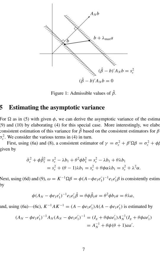
So the measurement-error corrected estimator cannot lie beyond the plane (βˆ − b)0ANb = sε2. This plane is parallel to the plane (βˆ −b)0ANb = 0, further away from the origin. The situation is illustrated in figure 1. The set ofβˆ’s compatible with  = φe1e01 is given by the line segment between the two planes, ranging fromb to

(βˆ−b)0ANb=0 (βˆ−b)0ANb=sε2 ANb b+λmaxa b

Figure 1: Admissible values ofβˆ.

5

Estimating the asymptotic variance

Foras in (5) with givenφ, we can derive the asymptotic variance of the estimators (9) and (10) by elaborating (4) for this special case. More interestingly, we elaborate consistent estimation of this variance forβˆbased on the consistent estimators forβ and σ_ε2. We consider the various terms in (4) in turn.

First, using (6a) and (8), a consistent estimator ofγ =σ_ε2+β0β = σ_ε2+φβ₁2is given by ˆ σ_ε2+φβˆ₁2=s_ε2−λb1+θ2φb21=s 2 ε −λb1+θ λb1 =sε2+(θ −1)λb1=sε2+θ φαλb1=sε2+λ 2 α. Next, using (6d) and (9),ω=K−1_{β =φ(A−φe}

1e0₁)−1e1e0₁βis consistently estimated by

φ(AN−φe1e10)− 1_e

1e01βˆ =θ φβˆ1a=θ2φb1a =θ λa, and, using (6a)—(6c),K−1_AK−1 _=(A−φe

1e10)A(A−φe1e01)is estimated by

(AN −φe1e01)− 1_A N(AN−φe1e01)− 1_=(I g+θ φae01)A− 1 N (Ig+θ φae01) =A−_N1+θ φ(θ+1)aa0.

Putting these results together gives forβˆ:

d

(asy.var.β)ˆ =(s_ε2+λ2α)(A_N−1+θ φ(θ+1)aa0)+θ2λ2aa0, (16) which of course reduces tos2

εA− 1

N when there is no measurement error.

6

The

t

-value for the first regression coefficient

For the estimator of the coefficient of the first regressor, taking the upper-left element in (16) gives d (asy.var.βˆ1)=(sε2+λ 2_{α)(α+θ φ(θ +1)α}2_)+θ2_λ2_α2 =θ2α(s2ε +2λ 2 α). Thet-statistic if there is no measurement error is

t0= b1 √ N p s2 εα , so s2ε = b2 1N t₀2α . (17)

Thet-statistic corresponding with a measurement error of sizeφ is, using (9) and (17), given by tφ = ˆ β1 √ N q d (asy.var.βˆ1) = θ b1 √ N θ√αps2 ε +2λ2α = t0 q 1+_N2h2 φ , (18)

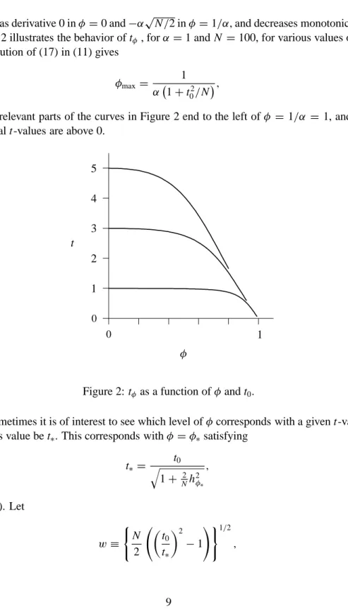
withhφ ≡λαt0/b1 =(θ −1)t0. After some straightforward calculations there appears to hold ∂tφ ∂φ = − 2 Nφ θ tφ 3 α2<0.

Sotφhas derivative 0 inφ =0 and−α

√

N/2 inφ =1/α, and decreases monotonically. Figure 2 illustrates the behavior oftφ, forα =1 andN =100, for various values oft0. Substitution of (17) in (11) gives

φmax=

1 α 1+t₀2/N,

so the relevant parts of the curves in Figure 2 end to the left ofφ =1/α = 1, and the minimalt-values are above 0.

0 1 φ 0 1 2 3 4 5 t

Figure 2:tφas a function ofφ andt0.

Sometimes it is of interest to see which level ofφcorresponds with a givent-value. Let this value bet_∗. This corresponds withφ =φ_∗satisfying

t_∗= q t0 1+_N2h2_φ∗ , (19) cf. (18). Let w≡ ( N 2 t0 t_∗ 2 −1 !)1/2 ,

then (19) implieshφ_∗ =wor φ_∗= 1 α w w+t0 .

In particular, one may be interested to see, by putting t_∗ at the conventional level of 2, what level of noise in a variable makes its estimated coefficient disappear into insignificance.

References

Bekker, P. A., Kapteyn, A., and Wansbeek, T. J. (1984). Measurement error and endogeneity in regression: bounds for ML and 2SLS estimates. In T. K. Dijkstra (Ed.), Misspecification analysis (pp. 85–103). Berlin: Springer.

Kapteyn, A., and Wansbeek, T. J. (1984). Errors in variables: Consistent Adjusted Least Squares (CALS) estimation. Communications in Statistics — Theory and Methods, 13, 1811–1837.

Krasker, W. S., and Pratt, J. W. (1986). Bounding the effects of proxy variables on regression coefficients. Econometrica, 54, 641–655.

Krasker, W. S., and Pratt, J. W. (1987). Bounding the effects of proxy variables on instrumental-variables coefficients. Journal of Econometrics, 35, 233–252. Lewbel, A. (1997). Constructing instruments for regressions with measurement error

when no additional data are available, with an application to patents and R & D. Econometrica, 65, 1201–1213.

Wansbeek, T. J., and Meijer, E. (in press). Measurement error and latent variables. In B. H. Baltagi (Ed.), Companion in theoretical econometrics. Oxford, UK: Basil Blackwell.