THREE PAPERS ON TIME SERIES FORECASTING
AND DATA PRIVACY
A Dissertation
Presented to the Faculty of the Graduate School of Cornell University
in Partial Fulfillment of the Requirements for the Degree of Doctor of Philosophy
by
Matthew J. Schneider May 2014
c
2014 Matthew J. Schneider ALL RIGHTS RESERVED
THREE PAPERS ON TIME SERIES FORECASTING AND DATA PRIVACY Matthew J. Schneider, Ph.D.
Cornell University 2014
The first paper applies receiver operating characteristic (ROC) analysis to micro-level, monthly time series of the M3-Competition. Forecasts from competing methods were used in binary decision rules to forecast exceptionally large de-clines in demand. Using the partial area under the ROC curve (PAUC) criterion as a forecast accuracy measure and paired-comparison testing via bootstrap-ping, we find that complex univariate methods perform best for this purpose. The second paper develops a multivariate forecasting model designed for fore-casting the largest changes across many time series. Using the partial area under the curve (PAUC) metric, our results show statistical significance, a 35 percent improvement over OLS, and at least a 20 percent improvement over competing methods. The third paper considers a particular maximum likelihood estimator (MLE) and a computationally intensive Bayesian method for differentially pri-vate estimation of the linear mixed-effects model (LMM) with normal random errors. The differentially private MLE performs well compared to the regular MLE, and deteriorates as the protection increases for a problem in which the small-area variation is at the county level. The direct Bayesian approach for the same model uses an informative, reasonably diffuse prior to compute the poste-rior predictive distribution for the random effects and the empirical differential privacy is estimated.
BIOGRAPHICAL SKETCH
Matthew J. Schneider is a Ph.D. Candidate in the Department of Statistical Sci-ence at Cornell University. He also holds a M.S. in Statistics from Cornell versity, a M.S. in Public Policy and Management from Carnegie Mellon Uni-versity, and a B.S. in Quantitative Economics from the United States Naval Academy. Previously, he was a Lieutenant in the U.S. Navy and policy analyst at the RAND Corporation.
ACKNOWLEDGEMENTS
I acknowledge NSF grants BCS 0941226, SES 9978093, ITR 0427889, and SES 0922005 for the funding of this work. I would also like to thank my coau-thors who provided an equal contribution to each of these papers. They in-clude Wilpen Gorr for the first two papers, and John Abowd and Lars Vilhu-ber for the third paper. Wilpen Gorr also served as my master’s advisor at Carnegie Mellon University and Lars Vilhuber served as an informal advisor at Cornell. Additionally, I really appreciate the insightful comments and guid-ance from my committee at Cornell University over the years. My committee members include Martin Wells, James Booth, Sachin Gupta, and John Abowd. John Abowd, based in the Department of Economics at Cornell University, is also my main advisor and has been extraordinary in his role advising me in or-der to complete the Ph.D. in Statistics. Martin Wells and James Booth, based in the Departments of Statistical Science and Biological Statistics and Compu-tational Biology at Cornell University, trained me in advanced statistical theory and methods and provided their great help to me since day one of the pro-gram. Sachin Gupta, based in the Marketing Department at Cornell University, has been instrumental in translating my statistical training to the marketing re-search community and continues to serve as a mentor to me. I am sincerely grateful.
CONTENTS
Biographical Sketch . . . iii
Acknowledgements . . . iv
Contents . . . v
List of Tables . . . vii
List of Figures . . . viii
1 Large-Change Forecast Accuracy: Reanalysis of M3-Competition Data Using Receiver Operating Characteristic Analysis 1 1.1 Introduction . . . 2
1.2 Literature Review . . . 5
1.2.1 M3-Competition data and forecast methods . . . 5
1.2.2 M3-Competition results . . . 6
1.2.3 ROC Statistical Tests . . . 7
1.3 Experimental Design . . . 8
1.3.1 Standardizing forecasted change and its gold standard . . 9
1.3.2 Gold standard cutoff . . . 10
1.3.3 Regression to the mean . . . 11
1.3.4 Forecast performance . . . 12
1.4 Results . . . 12
1.4.1 Partial Area Under Curve . . . 13
1.4.2 Complexity . . . 16
1.4.3 Decision-rule combination forecasts . . . 16
1.5 Conclusion . . . 19
2 ROC-Based Model Estimation for Forecasting Large Changes in De-mand 21 2.1 Introduction . . . 22
2.2 Management by Exception for Demand Forecasting . . . 24
2.3 Multivariate Leading Indicator Modeling . . . 29
2.3.1 PAUC Loss Function . . . 30
2.3.2 PAUC Maximization Forecast Model . . . 33
2.3.3 Comparison Models . . . 35
2.4 Empirical Application . . . 39
2.4.1 Data Source . . . 39
2.4.2 Gold Standard Policy . . . 40
2.4.3 Rolling Horizons . . . 41
2.4.4 Forecast Evaluation . . . 42
2.5 Results . . . 43
3 Differential Privacy Applications to Bayesian and Linear Mixed Model
Estimation 49
3.1 Introduction . . . 50
3.2 Data Sources . . . 53
3.3 Model Specifications . . . 55
3.3.1 Linear Mixed Model . . . 55
3.3.2 Bayesian Linear Mixed Model . . . 58
3.4 Differentially Private Estimation via Sub-sampling . . . 61
3.4.1 Sub-sampling . . . 61
3.4.2 Bias-correctedβˆ(i)anduˆ(i) . . . 62
3.4.3 Averaging Sub-samples as the Aggregation Function . . . 64
3.4.4 Number of Sub-samples . . . 67
3.4.5 Differentially Private Fitted Values . . . 67
3.5 Differentially Private Estimation via Expected Risk Minimization 69 3.5.1 Prior Specification . . . 71
3.5.2 Bayesian Computation and-Differential Privacy . . . 72
3.6 Results . . . 77
3.6.1 Linear Mixed Models . . . 77
3.6.2 Bayesian Linear Mixed Models . . . 83
3.7 Discussion . . . 84
3.8 Conclusion . . . 87
A Appendix for Paper 1 96 A.1 Standardizing forecasted change of M3-competition time series for ROC analysis . . . 96
LIST OF TABLES
1.1 Average rank of experts’ judgmental assessment of forecast
method complexity . . . 6
1.2 Best and worst forecast methods for M3 micro monthly time se-ries data (taken from Koning et al., 2005) . . . 7
1.3 Paired comparisons with the top forecasting method of PAUC for FPR range 0.0 to 0.2 using bootstrapping: one-step-ahead forecasts. . . 14
1.4 Kendall tau test . . . 16
1.5 Paired comparisons with the top forecasting method of PAUC for FPR range 0.0 to 0.2 using bootstrapping: one- and two-step-ahead forecasts for three rule-combination forecasts and their component forecast methods . . . 19
2.1 Summary Statistics of Crime Data . . . 40
2.2 Parameters Optimized Across Data Sets . . . 42
2.3 Five-Year ROC Curve for the Test Set . . . 45
2.4 Five-Year Correlation of Gold Standard to Forecasts, Test Set . . . 46
3.1 Technical Definitions . . . 91
3.2 Estimate Descriptions . . . 92
3.3 Maximum Empirical Ranges . . . 92
LIST OF FIGURES
1.1 ROC curves for a selection of M3-Competition methods, micro monthly time series, one- month ahead forecasts, 95% gold stan-dard cutoff. . . 17 2.1 Smoothed ROC Curves Over Five Years in Test Set . . . 44 2.2 Actual Violent Crimes for Two Census Tracts in the Test Set . . . 47 3.1 Equivalence table for optimalkover values offor JCR . . . 68 3.2 Trace Plots for County 1460. Panel A is the estimated random
effect for 10,000 MCMC samples, after burn-in, using all data and the first set of initial conditions. Panel B is the estimated random effect for 10,000 MCMC samples, after burn-in, using all data and the second set of initial conditions. . . 78 3.3 R-U Curve for JCR Linear Mixed Model with 49%budget forβ
and 49% foru . . . 85 3.4 R-U Curve for JCR Linear Model with 100%budget forβ . . . . 86 3.5 R-U Curve for JCR Linear Mixed Model with 88%budget forβ
and 10% foru . . . 87 3.6 R-U Curve for JCR Linear Mixed Model with 10%budget forβ
and 88% foru . . . 88 3.7 R-U Curve for JCR Linear Mixed Model with 97%budget forβ
and 1% foru. . . 89 3.8 R-U Curve for JCR Linear Mixed Model with 1%budget for β
and 97% foru . . . 90 3.9 R-U Curve for JCR Linear Mixed Model with 88%budget forβ
and 5% foruand 5% for interactions . . . 90 3.10 R-U Curve for JCR Linear Mixed Model with 97%budget forβ
and 0.5% foruand 0.5% for interactions . . . 93 3.11 Histogram for the Replicated Model Including All Observations
and Counties . . . 94 3.12 Histogram for the Model Deleting an Observation from County
CHAPTER 1
LARGE-CHANGE FORECAST ACCURACY: REANALYSIS OF M3-COMPETITION DATA USING RECEIVER OPERATING
CHARACTERISTIC ANALYSIS
This paper applies receiver operating characteristic (ROC) analysis to micro-level, monthly time series of the M3-Competition. Forecasts from competing methods were used in binary decision rules to forecast exceptionally large de-clines in demand. Using the partial area under the ROC curve (PAUC) crite-rion as a forecast accuracy measure and paired-comparison testing via boot-strapping, we find that complex univariate methods (including Flores-Pearce2, Forecast Pro, Automat ANN, Theta, and Smart FCS) perform best for this pur-pose. The Kendall tau test of dependency for PAUC and a judgmental index of forecast method complexity provides further confirming evidence. We also found that decision-rule combination forecasts using three top methods gener-ally perform better than the component methods, although not statisticgener-ally so. The top methods for forecasting large declines match the top methods for con-ventional forecast accuracy in the M3 Competition’s micro monthly time series. So evidence from the M3 competition suggests that practitioners use complex univariate forecast methods for operations-level forecasting, both for ordinary and large-change forecasts.
Key Words: Forecasting, ROC, M3-Competition, Exceptions Reporting, Large-Change Forecast Accuracy1 2
1Gorr, W. L. and Schneider, M. J. (2013). Large-Change Forecast Accuracy: Reanalysis of M3-Competition Data Using Receiver Operating Characteristic Analysis. International Journal of Forecasting, Vol. 29, Issue 2.
1.1
Introduction
According to the management by exception (MBE) principle (Taylor, 1911), operations-level staff should make resource-allocation decisions for production of goods or services under ordinary conditions; however, under exceptional conditions staff should defer to higher-level management. This approach makes the best use of top managers’ limited time, allowing them to deal with the dif-ficult cases and the broader lines of strategies and policy making. In the case of product or service demand forecasting, one type of exception is a forecasted large change from current demand. If a forecasted change exceeds a predeter-mined threshold level, then the demand forecasting system issues an exception report, calling for diagnosis by staff members and possible actions by upper management.
Gorr (2009) introduced receiver operating characteristic (ROC) curves as an accuracy framework for time series forecasting in support of MBE. The ROC framework analyzes the tails of forecast error distributions for exceptional de-mand conditions; whereas, traditional forecast error measures (such as the MAPE and MSE) place the most weight on the centers of forecast error dis-tributions and are best suited for ordinary demand conditions.
The “gold standard” for assessment of a forecast method in this paper is ac-tual change in demand, available ex post. For example, as a policy, managers may wish to review the top few percent of actual decreases (or increases) as de-fined by a cutoff quantile point of the gold standard distribution. If a decision rule’s threshold is crossed (i.e., the rule “fires”) and identifies an actual large change, the result is a “true positive,” otherwise it is a “false positive.” Other
outcomes are “true negative” where both forecasted and actual change are or-dinary and “false negative” where the actual change was large but forecasted change was ordinary.
Gorr (2009) defined gold standard values as those values extreme in regard to the standardized time series of data, for example, the top five percent of stan-dardized time series values. We can refer to this definition as “absolute” be-cause it references the entire time series, whereas the current paper’s definition is “relative” because it references only the last historical data point of a time se-ries. The absolute definition is preferable when there are large costs in adjusting from a baseline or average level of production. Here an example is neighbor-hood crime level where a flare up above the baseline crime pattern comes to the attention of news reporters. Increased fear and lost confidence in police by the public are large societal costs in addition to losses by crime victims.
The relative definition for time-series gold standards, introduced in this pa-per, is preferable in circumstances where there are high costs in changing the production technologies from current levels coupled with a potential for avoid-ing future costs of holdavoid-ing excess inventory or not meetavoid-ing customer demands. Examples are when additional machines need to be set up for increased de-mand or employees must be laid off for decreased dede-mand. Because the focus is on large changes from current production levels, the decision horizon must be for the very short term of one or two steps ahead and the first step ahead is the more important. For example, managers might expect large changes in six months or a year and be able to track and adjust to changes incrementally, but a large change in the next time period requires swift and substantial changes in plans.
This paper applies ROC analysis to M3-Competition data and its univariate forecast methods. A key question is whether complex univariate forecast meth-ods perform better than simple ones under ROC measures, similar to the case of Gorr (2009) who compared complex multivariate models to simple univari-ate methods for short-term forecasting and found complex methods to be more accurate. Most of the literature in the past 30 years supports using simple uni-variate methods for ordinary conditions (e.g., the M-competitions). This paper provides additional evidence that complex forecast methods are significantly more accurate than simple methods for exceptions forecasting, and specifically for univariate methods.
We also investigate whether a combination forecast leads to increased ac-curacy for exceptions forecasting. For forecasting ordinary conditions, combi-nations are averages or weighted averages of individual forecasts. In contrast, combination forecasts for exceptions use “or” or “and” logical connectors for individual-forecast-method decision rules. For example, the best-performing combination forecast method in this paper requires that any decision rule for component forecast methods fire (with “or” connectors) for the combination decision rule to fire.
Also new in this paper is application of the partial area under the ROC curve (PAUC) as the forecast accuracy measure for exceptions forecasting. Included is a statistical test for differences in PAUC using paired comparisons and account-ing for correlated data. The total area under the ROC curve has the interpreta-tion of being the probability that a decision rule will signal a randomly-chosen positive instance higher than a randomly chosen negative instance (Fawcett, 2006)
Section 2 provides a brief literature review of forecast error measures and competitions. Section 3 covers the experimental design for reanalysis of M3 data and Section 4 provides results. Finally Section 5 concludes the paper.
1.2
Literature Review
In this section we review the M3-Competition and its analysis of forecast accuracy, especially in regard to micro monthly time series. We also review the literature on statistical tests available for comparing ROC curves.
1.2.1
M3-Competition data and forecast methods
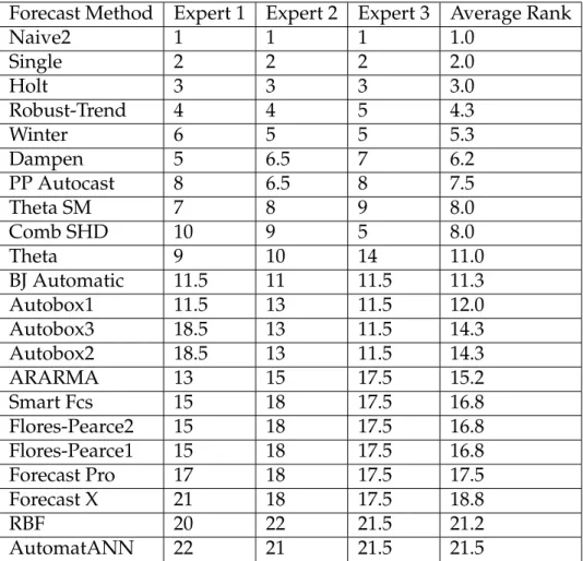
Operations and marketing managers forecast individual products or prod-uct families in an attempt to meet demand. Hence we limit this study to the micro, monthly time series of the M3-competition which best match this deci-sion setting. While both the M1 and M3 competitions have micro time series we use M3 data in this paper. The M3 competition has a wider range of univari-ate methods, especially more complex ones than M1. Furthermore, Koninget al.. (2005) provides judgmentally-derived complexity ranks for the M3 forecast methods made by three forecasting experts, which we relate to forecast accu-racy. We averaged the complexity ranks across the experts and rescaled ties to yield the average ranks in Table 1.1. To learn more about the forecast methods in Table 1.1, see Table 1.2 in Makridakis & Hibon (2000, p 456).
Forecast Method Expert 1 Expert 2 Expert 3 Average Rank Naive2 1 1 1 1.0 Single 2 2 2 2.0 Holt 3 3 3 3.0 Robust-Trend 4 4 5 4.3 Winter 6 5 5 5.3 Dampen 5 6.5 7 6.2 PP Autocast 8 6.5 8 7.5 Theta SM 7 8 9 8.0 Comb SHD 10 9 5 8.0 Theta 9 10 14 11.0 BJ Automatic 11.5 11 11.5 11.3 Autobox1 11.5 13 11.5 12.0 Autobox3 18.5 13 11.5 14.3 Autobox2 18.5 13 11.5 14.3 ARARMA 13 15 17.5 15.2 Smart Fcs 15 18 17.5 16.8 Flores-Pearce2 15 18 17.5 16.8 Flores-Pearce1 15 18 17.5 16.8 Forecast Pro 17 18 17.5 17.5 Forecast X 21 18 17.5 18.8 RBF 20 22 21.5 21.2 AutomatANN 22 21 21.5 21.5
Table 1.1: Average rank of experts’ judgmental assessment of forecast method complexity
1.2.2
M3-Competition results
A major conclusion of the M3-Competition is “Statistically sophisticated or complex methods do not necessarily produce more accurate forecasts than sim-pler ones” (Hibon & Makridakis, 2000, p 458). Micro monthly data, however, are a case for which complex forecast methods are more accurate than simple ones. For example, Table 1.2 summarizes best and worst performing methods for micro monthly data according to four forecast error measures used in the M3-competition (Koning et al.. 2005). All of the best methods are complex except for Theta, which has mid-range complexity. All of the worst methods
are simple, except Box Jenkins methods which also have mid-range complexity. Apparently micro monthly time series data have patterns that complex methods are able to estimate and make good use of under ordinary conditions. The ques-tion is whether complex models are also better for excepques-tional condiques-tions. For example, when change is in progress neural networks have pattern recognizers that can turn on model components selectively to capture and extrapolate the change and expert systems can switch to more reactive models.
Error Measure Best Four Forecast Methods (in order)
sMAPE SmartFCS, Theta, AutomatANN, ForecastPRO Median sAPE SmartFCS, Theta, AutomatANN, ForecastX RMSE Theta, SmartFCS, ForecastX, ForecastPRO Error Measure Worst Four Forecast Methods (in order) sMAPE Robust-Trend, Naive2, Single, ARARMA Median sAPE Robust-Trend, Naive2, ARARMA, Single RMSE Robust-Trend, Naive2, RBF, Autobox
Table 1.2: Best and worst forecast methods for M3 micro monthly time se-ries data (taken from Koning et al., 2005)
1.2.3
ROC Statistical Tests
Cohen et al.. (2009) and Gorr (2009) provide reviews of ROC curves and analysis applied to time series data monitoring and forecasting respectively. Hence this section only summarizes the ROC literature in regard to additional material on statistical tests introduced in this paper for time series testing.
Area under curve (AUC) is the total area under an ROC curve over the entire false positive rate (FPR) range of 0 to 1. The higher the AUC, the better the forecasting method (or other test mechanism). AUC can be computed using the
the nonparametric Wilcoxon statistic, as shown by Hanley and McNeil (1982). The Wilcoxon statistic can be used to calculate the standard error of the AUC for statistical tests (Hanley and McNeil, 1982). Alternatively, the standard error and AUC can be determined using the DeLong, DeLong, & Clarke-Pearson (1988) method.
Partial area under curve (PAUC) is the area under an ROC curve for a speci-fied FPR range, generally starting at zero. In many situations, a decision maker has a maximum FPR threshold which he or she is not willing to exceed and PAUC represents this case. PAUC can be computed using the trapezoidal rule and bootstrapping can be used to compute its standard error.
Parametric and nonparametric statistical tests for comparing the AUCs of two ROC curves with correlated data are described by Hanley and McNeil (1983). Forecasting competitions generally have correlated data because alter-native forecast methods are applied to the same cross section of time series. The available tests require standard errors calculated by the Dorfman and Alf (1969) maximum likelihood program or the Wilcoxon statistic and a correlation co-efficient calculated by the Pearson product-moment correlation method or the Kendall tau rank correlation coefficient. Bootstrapping removes the need for a covariance estimate and accounts for correlated data (Janes, Longton, & Pepe, 2009).
1.3
Experimental Design
We used ROC analysis to study large-change forecast accuracy for one- and two-month-ahead forecasts. This section describes how we processed the 474
time series of the M3 micro monthly data to create empirical ROC curves. The time series tend to be declining at the forecast origin, so we focused on excep-tional declines—certainly a major concern of managers in firms selling products or services.
Included in this section is how we standardized data to facilitate cross-sectional specification of decision rule limits as well as how we tabulated results to produce ROC curves.
1.3.1
Standardizing forecasted change and its gold standard
Following is notation for the time series, forecasts, time series changes, and forecasted change.
Cross section of actual time series:
Yit(i= 1, . . . I;t= 1, . . . T+m)whereiis a time series,tis time;T is the single,
fixed forecast origin of the M3-Competition; and m is the forecast horizon (here we usem = 1and2only)
Set of alternative forecast methodsj = 1, . . . , J and forecasts: Fijt(i= 1, . . . I;j = 1, . . . J;t=T +m)
Forecasted change:
F orecastDeltaijT+m =FijT+m−YiT(i= 1, . . . I;j = 1, . . . J;m = 1or2)
realization in the estimation data set:
DeltaiT+m =YiT+m−YiT(i= 1, . . . I;m= 1or2)
We need to standardize each ForecastDelta and Delta to remove scale and control variation, analogous to computing z-scores. Then we can use the same standardized threshold values of decision rules for each time series (as is done with t-statistics or normal tables). While we can estimate the sample mean and standard deviation for Deltas, there is a limitation in standardizing Forecast-Delta. The M3-competition had a single forecast origin for each time series and a single set of corresponding forecasts for m = 1, . . . ,18, so there is only a sample of size one for eachFijT+m. If the competition had used a rolling or
expanding horizon design with many forecast origins, we could estimate the mean and standard deviation of ForecastDelta for each series andm. However for the M3-Competition we must use an approximation, which is facilitated by the way ROC curves are constructed. We need only assume that ForecastDeltas are proportional to Deltas by forecast method in the sample of time series. Then we can normalize ForecastDeltas by the mean and standard deviation of the deltas (see the Appendix).
1.3.2
Gold standard cutoff
Deltas that were a specified number of standard deviations below the mean were considered true large change values (“positives” in regard to ROC). We specified three cutoffs of -1.28, -1.65, and -2.33 standard deviations below the mean corresponding to 10%, 5%, and 1% quantile points of the delta distribu-tion if it were normally distributed. For first differences (DeltaiT+1) of the 474
time series, there are 110, 74, and 24 positives for the 10%, 5%, and 1% cutoffs respectively. For second differences (DeltaiT+2), the corresponding number of positives are 89, 57, and 27. Even after removing spurious, regression-to-the mean cases in Section 3.3, the numbers of positives are higher than for a normal distribution because of the “fat” lower tail (and thin upper tail) of the distribu-tion and also because our standardizadistribu-tion is approximate. Regardless, it is im-portant to analyze more than one gold-standard cutoff to examine how forecast performance varies with the definition of positives. For example, Gorr (2009) found ROC performance to improve with more extreme definitions, likely be-cause the most extreme cases are the easiest to distinguish from the rest of the distribution.
1.3.3
Regression to the mean
It is necessary to control for regression-to-the-mean behavior in the case when exceptional values do not persist (i.e., they are outliers) and time series patterns return to the mean of the series. For large declines, the problem occurs when the time series has a high outlier that returns to the mean. Take the case of one-step-ahead forecasts. Any non-responsive forecast method or model has good performance for the data point following the outlier, spuriously inflating AUC or PAUC measures. The actual data point returns to the mean while the unresponsive forecast method never left the mean. SoF orecastDeltaijT+1 fires a decision rule, testing positive, andDeltaiT+1 is a positive yielding a spurious true positive. The same is true form-step-ahead forecasts,m steps after an in-creasing outlier. The one-step-ahead forecasts for the three thresholds of -1.28,
respectively. The two-step-ahead forecasts have 30 out of 89, 15 out of 57, and 3 out of 23 regression cases. We excluded forecasts, and therefore corresponding time series, affected by regression to the mean from our analyses.
1.3.4
Forecast performance
For every threshold, standardized ForecastDeltas less or equal to the z-value threshold were considered to signal a large decrease (test positive). Fore-casts methods with test positives in a series that had an actual positive are true positives. Otherwise, the forecast method provided a false positive. This pro-cess was repeated for a maximum of 475 z-value thresholds occurring at the boundaries of the 474 ranked normalized ForecastDeltas, thus spanning all pos-sibilities for the construction of ROC curves.
True Positive Rates (TPRs, number of true positives divided by number of positives) and False Positive Rates (FPRs, number of false positives divided by number of negatives) were computed to obtain increasing two-dimensional points (FPR, TPR) for each method. The connection of these points created each method’s empirical ROC curve and statistical tests were applied from Section 2.
1.4
Results
We decided to limit analysis to the PAUC measure for false positive rates be-tween 0.0 and 0.2, believing that this would include the range in which most managers would be comfortable operating. Note that it is common in practice to use larger false positive rates (which are the same as type I error rates) than
used in theory testing (e.g., see Cohen, et al.., 2009) depending on the cost of false negatives, prevalence of positives, and resources available for diagnosis and follow-up to test positives.
1.4.1
Partial Area Under Curve
We compare large-change forecast performance of forecast methods using a non-parametric bootstrap approach for paired comparisons between PAUCs. One sided p-values were computed for each PAUC threshold’s top performing method to see whether it was statistically better than other methods. We use 1,000 bootstrap samples for each pair of methods.
See Table 1.3 for results at the 0.05 significance level for one-step-ahead fore-casts over the FPR range of 0.0 to 0.2. We only included methods in the com-parison that have complexity scores in Table 1.1 (dropping AAM1 and AAM2) and in addition we dropped Rule-Based Forecasting because it was designed for annual data and we are analyzing monthly data.
In general, complex methods performed significantly better than simple methods. Automat ANN, Flores-Pearce2, Forecast Pro, Smart FCS, and Theta were in the set of methods either best or not significantly different from the best for all three cutoff points used for gold standards. All but Theta are complex methods with subjective scores from Table 1.1 at 16.8 or higher. Theta has mid-range complexity with a score of 11.0. SmartFcs, with a complexity score of 16.8, was in the significantly better methods for the 95% and 90% gold standard cutoffs, and BJ automatic (mid-range complexity score of 11.3) joins the
signif-more extreme the positive cases are (i.e., the more stringent the gold standard cutoff), the better the PAUC performance which is similar to findings by Gorr (2009).
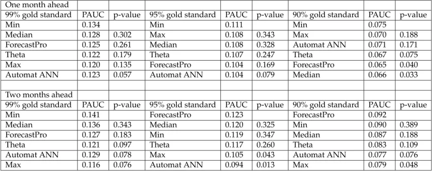
99% gold standard PAUC p-value 95% gold standard PAUC p-value 90% gold standard PAUC p-value
Flores/Pearce 2 0.145 Theta 0.107 Automat ANN 0.071
Automat ANN 0.123 0.112 Automat ANN 0.104 0.396 SmartFcs 0.069 0.431
Theta 0.122 0.086 Forecast Pro 0.104 0.374 Theta 0.067 0.275
ForecastPro 0.125 0.082 SmartFcs 0.102 0.315 ForecastPro 0.065 0.225
Dampen 0.112 0.045 Flores/Pearce 2 0.100 0.210 Flores/Pearce 2 0.065 0.203
Single 0.104 0.024 Theta sm 0.088 0.017 BJ automatic 0.059 0.080
SmartFcs 0.119 0.021 BJ automatic 0.089 0.015 Forecast X 0.056 0.044
Autobox2 0.099 0.016 ARARMA 0.081 0.008 Naive 2 0.048 0.028
Holt 0.101 0.015 PP-autocast 0.089 0.005 ARARMA 0.053 0.026
PP-autocast 0.105 0.010 Forecast X 0.084 0.005 Dampen 0.054 0.021
Winter 0.099 0.010 Flores/Pearce 1 0.084 0.004 Flores/Pearce 1 0.054 0.018
ForecastX 0.100 0.008 Autobox2 0.078 0.002 PP-autocast 0.053 0.014
BJ automatic 0.098 0.003 Dampen 0.083 0.002 Autobox3 0.049 0.014
Flores/Pearce 1 0.099 0.003 Autobox3 0.075 0.001 Robust-Trend 0.043 0.012
ARARMA 0.085 0.003 Holt 0.072 0.000 Theta sm 0.052 0.012
Naive2 0.076 0.001 Winter 0.070 0.000 Autobox2 0.051 0.008
Theta-sm 0.089 0.000 Single 0.070 0.000 Holt 0.044 0.002
Autobox3 0.074 0.000 Autobox1 0.062 0.000 Winter 0.042 0.001
Autobox1 0.059 0.000 Naive2 0.053 0.000 Single 0.038 0.000
Robust -Trend 0.025 0.000 Robust-Trend 0.040 0.000 Autobox1 0.035 0.000
Table 1.3: Paired comparisons with the top forecasting method of PAUC for FPR range 0.0 to 0.2 using bootstrapping: one-step-ahead forecasts.
For the two-step-ahead forecasts, the significantly better forecasting meth-ods (in decreasing order of PAUC values) are as follows:
99% gold standard: Automat ANN, Theta sm, Flores/Peacre2, ForecastPro, BJ automatic, Theta, SmartFcs, and Autobox2
95% gold standard: ForecastPro, Flores/Pearce 2, Theta sm, Theta, SmartFcs
ahead forecasts but Theta sm and Autobox 2 show up as new for two-step-ahead forecasts. Flores/Pearce 2 and Forecast Pro are in every significantly better set while Smart Fcs is close behind in all but one of those sets.
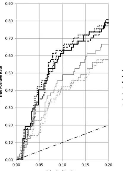
A ROC curve is a plot of true positive rate (TPR) versus false positive rate (FPR) obtained by varying the threshold level of an exceptions decision rule. Figure 1.1 displays a selection of ROC curves for one-step-ahead forecasts and the 95% gold standard case from Table 1.3. ROC curves for other cases are sim-ilar qualitatively. Shown are three top-performing methods (all complex) and three simple smoothing methods. Also shown is the line representing a chance decision mechanism.
For a given FPR, the method with the highest ROC curve is best, having the highest TPR. At 0.01 FPR there is no difference in performance but by 0.05 FPR the complex methods have a TPR range of approximately 0.32 to 0.42 while the simple methods have a range of 0.15 to 0.28. At 0.10 FPR, the complex methods have a TPR range of 0.61 to 0.63 while the simple methods only have a range of 0.40 to 0.49. So the complex methods have much better performance than the simple methods. At the maximum FPR rate in Figure 1.1 the best method finds just over 80 percent of the positive cases (gold standard large decreases). Note that Dampen has better performance than Single or Holt because, as shown by Snyder & Koehler (2008), it “. . . possesses a special capacity to adapt to struc-tural change without direct intervention.”
1.4.2
Complexity
This section investigates the effect of forecast method complexity on ROC performance, measured by PAUC, over the M3 micro monthly time series. We eliminated Rule-Based Forecasting from the analysis because it is an annual time series method, whereas the micro-level data analyzed in this paper are monthly. We also dropped the Na¨ıve method because it yields 0 change comparing fore-casts to last historical value and the AAM1/AAM2 methods which were not ranked by the experts for complexity in Table 1.1. We expected the relationship between complexity and PAUC to be positive.
Table 1.4 contains the results of applying Kendall’s tau with a two-sided test and 0.05 significance level in regard to the dependence of PAUC for the FPR range of 0 to 0.20 on average rank for complexity in Table 1.1. Cases included are the three gold-standard cutoffs for defining positives and one- and two-month ahead forecasts. Five out of six cases have significant tests at the 0.05 level or better, thus providing further evidence that the complex forecast methods are best for the large-change forecast accuracy for the M3 micro monthly time series
99% gold standard 95% gold standard 90% gold standard
One step ahead tau = 0.197 p-value=0.241 tau = 0.464 p-value =0.005 tau = 0.535 p-value =0.001 Two steps ahead tau = 0.432 p-value =0.009 tau = 0.379 p-value =0.023 tau = 0.411 p-value =0.013
Table 1.4: Kendall tau test
1.4.3
Decision-rule combination forecasts
It is well-known that a simple average combination of methods’ forecasts often forecasts more accurately than the component methods (e.g., Clemen,
Figure 1.1: ROC curves for a selection of M3-Competition methods, mi-cro monthly time series, one- month ahead forecasts, 95% gold standard cutoff.
1989). We propose combination forecasts for exceptions forecasting that com-bine decision rules instead of forecasts. For a decision-rule combination forecast with a fixed number of component forecast methods, if a prescribed number of component methods’ rules fire (test positive), then the composite decision rule fires. The benefit of such a rule could be to make more conservative decisions,
positives—depending on whether “and” or “or” logical connectors are used for component rules.
We created three combination forecasts, each with the same three top-performing, complex forecast methods: ForecastPro (expert system), Automat ANN (neural network), and Theta (decomposition method). Because each of the component methods have different modeling approaches, this combination promises to maximize information available for forecasting exceptions. The first combination rule (Min) has test positives whenever any of the three component methods has a test positive. The second (Median) is a median combination fore-cast that has test positives whenever two of the three component methods had a test positive. Finally, the third (Max) that has test positives when all of the top three methods have a test positive.
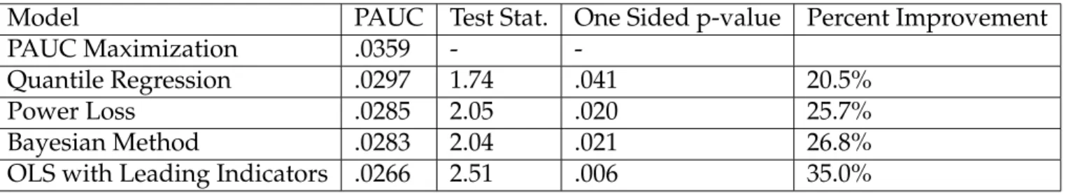
Table 1.5 has the results, using the same paired comparison test as in Table 1.3. Here we limit the comparisons to the three combinations as well as their three component forecast methods to see if combinations can improve forecast accuracy over components. The liberal Min combination is best for all three one-month-ahead cases and one of the three two-month cases, but is not significantly so at the 0.05 significance level. ForecastPro is best in the other two two-month-ahead cases. Thus rule-combination forecasts are promising: for forecasting large changes for important micro monthly time series, we recommend the Min rule-combination forecast.
One month ahead
99% gold standard PAUC p-value 95% gold standard PAUC p-value 90% gold standard PAUC p-value
Min 0.134 Min 0.111 Min 0.075
Median 0.128 0.302 Max 0.108 0.343 Max 0.070 0.188
ForecastPro 0.125 0.261 Median 0.108 0.328 Automat ANN 0.071 0.171
Theta 0.122 0.179 Theta 0.107 0.247 Theta 0.067 0.075
Max 0.120 0.135 ForecastPro 0.104 0.169 ForecastPro 0.065 0.040
Automat ANN 0.123 0.057 Automat ANN 0.104 0.079 Median 0.066 0.033
Two months ahead
99% gold standard PAUC p-value 95% gold standard PAUC p-value 90% gold standard PAUC p-value
Min 0.141 ForecastPro 0.123 ForecastPro 0.092
Median 0.136 0.343 Median 0.120 0.325 Min 0.090 0.389
ForecastPro 0.127 0.183 Min 0.119 0.347 Median 0.087 0.188
Theta 0.121 0.097 Theta 0.117 0.260 Theta 0.083 0.109
Automat ANN 0.129 0.078 Max 0.105 0.043 Automat ANN 0.077 0.076
Max 0.116 0.076 Automat ANN 0.094 0.013 Max 0.079 0.048
Table 1.5: Paired comparisons with the top forecasting method of PAUC for FPR range 0.0 to 0.2 using bootstrapping: one- and two-step-ahead fore-casts for three rule-combination forefore-casts and their component forecast methods
1.5
Conclusion
This paper applied ROC analysis to the M3-Competition’s micro monthly time series for one- and two-month-ahead forecasts. Using the partial-area-under-the-curve (PAUC) criterion, paired comparison testing via bootstrapping, and the Kendall tau we found that complex methods perform best for fore-casting large declines in these time series, which tended to decline as a group over time. The classification of top methods matches that obtained using con-ventional forecast accuracy methods in the M3 Competition: complex methods forecast these series better than simple ones.
We also found that a rule-combination forecast, requiring that any of three decision rules of the combination methods fire to produce a test positive, to
perform better than the component methods but not with statistical significance.
Thus the evidence from the M3 competition suggests that operations man-agers should use complex methods such as Theta, a neural network, Forecast-Pro, or SmartFcs for forecasting both ordinary and large-change demand data.
CHAPTER 2
ROC-BASED MODEL ESTIMATION FOR FORECASTING LARGE CHANGES IN DEMAND
Forecasting for large changes in demand should benefit from different esti-mation than that used for estimating mean behavior. We develop a multivari-ate forecasting model designed for forecasting the largest changes across many time series. The model is fit based upon a penalty function that maximizes true positive rates along a relevant false positive rate range and can be used by managers wishing to take action on a small percentage of products likely to change the most in the next time period. We apply the model to a crime dataset and compare results to OLS as the basis for comparisons as well as models that are promising for large-change demand forecasting such as quantile regression, synthetic data from a Bayesian model, and a power loss model. Using the par-tial area under the curve (PAUC) metric, our results show statistical significance, a 35 percent improvement over OLS, and at least a 20 percent improvement over competing methods. We suggest managers with large numbers of time se-ries (e.g., for product demand) to use our method for forecasting large changes in conjunction with typical magnitude-based methods for forecasting expected demand.
Keywords: Management By Exception, PAUC Maximization, Large Changes, Forecasting Exceptions, ROC Curves. 1 2
1Coauthored with Wilpen L. Gorr
2.1
Introduction
Demand forecasting generally is done with extrapolative time series meth-ods, such as exponential smoothing with level, trend, and seasonal compo-nents. Time periods during which the underlying univariate model is stable and forecast accuracy is acceptable are called “business as usual” (BAU) in this paper. Highly disaggregated time series, such as for product or service demand, however are notorious for having large changes—outliers, step jumps, turning points, etc.— that cannot be forecasted using simple extrapolative forecast mod-els. Thus the time series forecasting field has long recognized the importance of handling exceptions to BAU; in particular, by developing time series monitoring methods for early detection of large changes (e.g., Brown, 1959; Trigg 1964).
Time series monitoring supports reactive decision making, after large changes have occurred. Better, if forecast models are accurate enough, is to fore-cast large changes in demand to allow proactive decision making, with a chance of preventing losses or taking advantages of potential gains. This paper pro-poses a new estimation method for forecast models aimed at improving forecast accuracy for large changes in demand. The new estimation method minimizes a loss function based on a receiver operating characteristic (ROC) measure, par-tial area under the ROC curve (PAUC). Section 2 reviews the underlying deci-sion framework—management by exception (MBE)—and ROC methods used to implement MBE for large-change demand forecasting, including PAUC. Es-sentially, ROC assesses predictions for binary classification, in the case of this paper that a future period will or will not have a large increase or decrease in demand.
While central-tendency forecast error measures, such as MAD, MAPE, and MSE, are best for evaluating forecast accuracy under BAU, recent research shows that a different kind of forecast error measure is needed for evaluation under large-change conditions for demand. Gorr (2009) compared univariate versus multivariate forecast models using the same data and found that forecast performance assessed using MAPE strongly favored simple univariate meth-ods, whereas ROC assessment strongly favored the multivariate model. The multivariate model had leading indicator independent variables capable of fore-casting large changes when there were large changes in lagged leading indi-cators. Gorr & Schneider (2013) compared simple versus complex univariate forecast models for large changes using monthly data from the M3 competition and found that PAUC assessments for large-change forecasts showed that the complex univariate models are significantly more accurate than simple univari-ate models. Apparently, complex univariunivari-ate models have enough additional parameters in functional forms to make them sensitive to subtle indications of rapidly changing trends.
Parker (2011) goes a step further and shows that classification performance over seven measures of classification (which included AUC but not PAUC) is best by picking the right performance measures as a loss function for estima-tion. In line with this result, this paper provides evidence that parameter esti-mates for a multivariate forecast model made using the PAUC, ROC-based loss function are much more accurate for large-change demand forecasts than those from a central-tendency-based loss function (MSE). To our knowledge, there is no previous empirical research in time series forecasting using a ROC-based loss function for model estimation.
The general point of the emerging literature on large-change demand fore-casting, including this paper, is that an organization can continue to use what-ever extrapolative forecast models it prefers for BAU, but it needs a second, pre-emptive forecast model that takes over for large demand changes. Needed are two kinds of forecast accuracy measures (central tendency for BAU magnitudes and PAUC for classification), two kinds of forecast models (simple extrapolative for BAU and complex univariate or multivariate for MBE), and two kinds of loss functions for forecast model estimation (central tendency for BAU magnitudes and PAUC for MBE classification).
Section 2 provides motivation and background for the paper’s new estima-tion method with an overview of MBE and ROC applied to large-change fore-casting. Section 3 develops the ROC-based method for parameter estimation for a multivariate, leading indicator forecast model and develops comparison models. Section 4 describes the time series data used to calibrate the model and rolling horizon forecast experiment. Section 5 presents results comparing alter-nate forecast models with significance testing. Finally, section 6 concludes the paper with a summary and suggestions for future work.
2.2
Management by Exception for Demand Forecasting
This section provides an overview of MBE implemented with ROC analy-sis as applied demand forecasting. MBE and ROC provide a decision-making framework, model, and methods for managing exceptional, large-change de-mand conditions. The large literature on optimal inventory control models (e.g., Brown, 1959) provides corresponding methods for BAU conditions, but
mod-els and methods for large-change conditions are fairly new. The key to success in this area is getting accurate forecasts, tuned for the tails of demand distri-butions, and that is the purpose of this paper, to the provide new estimation methods for large-change demand conditions.
MBE depends on the decision of whether or not to flag a forecast as being large-change, implemented via decision rules analogous to hypothesis testing, except that decision-rule thresholds cannot use the traditional Type I (false pos-itive) error rates of empirical research (1 or 5 percent). Instead a false positive rate and corresponding decision-rule threshold must be determined based on cost/benefit considerations. ROC provides the decision model and methods for determining optimal false positive error rates, and corresponding decision rule thresholds.
MBE, one of the oldest forms of a management control system (Taylor, 1911; Ricketts & Nelson, 1987), provides the principle that only variances (exceptions) from usual conditions should be brought to managers’ attention. All else should be handled by operational staff using standard procedures. Then managers’ limited time can be devoted to decisions requiring their expertise and power on emerging problems or opportunities. One type of variance is a large change in demand for products or services (West et al., 1985; Gorr, 2009; Gorr & Schnei-der 2013). Demand is only partially affected by an organization’s efforts, given competition in the market place, limits of marketing programs, and changing consumer tastes. Hence, large changes in demand are an important source of variances for triggering MBE reports to production and marketing managers. MBE can be reactive, based on detection with time series monitoring methods, or proactive, based on forecasting. First we discuss detection and then move on
to forecasting.
Time series monitoring methods, such as the Trigg (1964) and Brown meth-ods (1959), compute a test statistic used in a decision rule analogous to hypoth-esis testing, for making the binary decision. The decision rule uses a threshold value, if exceeded by the test statistic, is a signal trip or “yes,” otherwise the de-cision is “no” there is no large change. If “yes” then the time series undergoes diagnosis, using additional data and expertise, to determine if any interven-tion is needed into BAU practices (e.g., a new marketing plan, price decrease, product improvements, or decreased production level). Next we discuss the mechanics of implementing such decision rules using ROC.
There needs to be an external determination as to when a time series has data points considered in fact to be large changes. Such a data point is called a “positive” and is determined by a “gold standard.” All other time periods are “negatives.” In public health, where ROC is used extensively (e.g., Pepe, 2004), the analogous problem to MBE for demand forecasting is population screening for sick individuals. To be economically feasible, screening must use inexpen-sive and therefore imperfect tests, but then for individuals flagged as possibly sick, one needs a “gold standard” test for determining whether individuals are really sick or not, one that generally is expensive and more invasive. For ex-ample, for prostate and breast cancer screening, the gold standard is biopsy, examining sample tissue under a microscope. Biopsy is not infallible, but is much more accurate than screening tests such as PSA level in blood samples for screening prostate cancer.
Of course, the demand forecasting problem does not have gold standard tests, such as biopsy, for large demand changes. Instead, managers must use
judgment to determine changes large enough to be worth the cost of diagnosis and possible action. Gorr (2009) used a gold standard policy, that the top small percentage of large changes in standardized time series data be considered pos-itives, and reasoned that police officials have means to make such judgments (e.g., police would like to prevent the large changes that are reported in the news media). This gold standard is applied to out-of-sample forecasts during the evaluation stage, when actual values are available. A gold standard pol-icy avoids the alternative of applying expertise and judgment to all time series points individually to determine positives in the evaluation phase of forecast-ing. Cohenet al.(2009) took this alternative, and while effective, was very costly.
There are four outcomes for a binary decision: true positive (the signal trips and the time period is a positive), false positive (the signal trips but the time period is a negative), false negative (the signal does not trip but the time period is a positive), and true negative (the signal does not trip and the time period is a negative). Application of a decision rule with a given threshold in repeated trials over time and across time series is summarized using a contingency (or confusion table) with frequency counts of all four possible outcomes. Common statistics from this table are the true positive rate, TPR = number of true posi-tives/number of positives, and false positive rate, FPR = number of false pos-itives/number of negatives. The complements of these statistics are the false negative rate and true negative rate.
It is a fact that increasing the true positive rate necessarily increases the false positive rate, so that there is a trade-off to be made in determining an optimal, corresponding decision-rule threshold. This is seen in the shape of the ROC curve, which plots true positive rate versus false positive rate for all possible
decision rule thresholds and is an increasing function with decreasing slope be-tween (0,0) and (1,1). The higher the ROC curve for a model, the more accurate the binary decision model. An overall measure of the performance of a moni-toring or forecast model thus is area under the ROC curve (AUC) which ranges between 0 and 1. Better in practice is partial area under the ROC curve (PAUC). This is the area for a restricted range of false positive rates, often from 0 up to 10 or 20 percent because the cost of processing signal trips for false positive rates exceeding those rates generally is excessive and/or beyond available resources. See Figure 2.1 in section 5 for example ROC curves and to get a sense of the kind of time series data being forecasted in this paper.
Empirical research uses traditional values, such as 1 or 5 percent, for false positive rates (Type I errors) that determine decision rule thresholds from nor-mal or t-distribution tables. This practice implements a conservative view on accepting evidence of new theories. Business, however, needs to determine thresholds to obtain the optimal trade-off of true versus false positive rates. It is straightforward to write a utility model for the binary decision problem and to derive optimality conditions (e.g., see Metz, 1978; Cohen et al., 2009). The op-timal false positive rate is determined by finding the point at which a derived straight line is tangent to the ROC curve. The slope of that line depends on the prevalence of positives and the ratio of the utility of avoiding a false negative versus the utility of avoiding a false positive. For example, Pittsburgh police of-ficials estimated that it is 10 times more important to avoid a false negative than a false positive when monitoring serious violent crimes for large increases, and this led to a 15 percent false positive rate as optimal for time series monitoring (Cohen et al., 2009). Likewise, population screening for prostate and breast can-cers have false positive rates roughly in the range of 10 to 15 percent for most
parts of the world (e.g., Banez et al., 2003; Elmore et al. 2002). In both crime and public health cases, the severe consequences of false negatives (not intervening when there is a large increase in serious violent crime or not catching cancer in early stages) outweighs the costs of processing false positives. So-called ”A” items from ABC inventory analysis (e.g., Ramanathan, 2006) are likely similar in terms of importance or consequence.
All of the framework and methods discussed in this section depend on being able to forecast large changes accurately enough. Thus the next section of this paper develops a model estimated using a loss function based on PAUC to best tune model parameters for MBE.
2.3
Multivariate Leading Indicator Modeling
Multivariate leading indicator models that restrict forecasting to linear pre-dictors of the form
ˆ
y=Xβˆ (2.1)
are compared. yis the dependent vector with observationsyi fori= 1, ..., n
and X is the matrix of leading indicators (with time lagged values) with rows xi. All models estimate βˆ in-sample on different loss functions L which are
functions of the data (y and X). Proposed models are well suited for large-change forecasting and central tendency models (ordinary least squares) pro-vide a benchmark. First, the PAUC loss function is formally developed, then the
comparison models.
For all modeling, we define the initialization set as the set of data which is used to estimateβˆand not used in forecasting. The training set is is the set of data used for model selection based on pairwise comparison of out-of-sample results in the training set only. The test set is the set of data used to evaluate all models in this paper and report the results. This paper uses rolling horizon forecasts and iteratively conditions on all data up to time t to forecast data in timet+ 1. We define in-sample data as data up to time periodtthat is used to forecast out-of-sample data in time periodt+ 1. Depending on the time period, in-sample data can exist in both the training and test sets, however pairwise comparisons for metaparameter selection are only performed in the training set (using the PAUC loss function as the comparison) and results are only reported for the test set. Both of these are done using out-of-sample forecasts only. See Table 2.2.
2.3.1
PAUC Loss Function
This section develops the functional form of the 1-PAUC loss function used for estimation. A manager states the gold standard policy that transforms the decision variable,y, into a binary gold- standard vector,g, where a 1 indicates a positive and a 0 indicates a negative,
y∈Rn −→g∈ {0,1}n
(2.2)
inter-vention, that we want to have flagged by a forecast. The policy is implemented using a threshold, not to be confused with decision-rule thresholds discussed below, for standardized values of the dependent variable, y∗, in our empirical application. Standardization matches the police criterion of equity for allocating resources to different regions of a city. If raw crime counts were used, all extra police resources would be allocated to the highest crime areas; whereas, with standardized crime counts any area, regardless of crime scale, with a relatively large increase in crime can get extra police resources. Section IV has details on the gold standard used in this paper.
ROC curves plot TPR versus FPR for all possible decision-rule thresholds of a given set of forecasts. ROC curves are constructed by comparing the rank of all forecasts to the gold standard vector. For forecast valuesyˆi =Xiβˆ, define the
jthdecision rule threshold,j = 1,2, ...,(1+number of uniqueyˆi’s) corresponding
to selected constantscj’s which divide the ranked yˆi’s. Then, a decision rule is
defined under thejth threshold andithobservation where 1
ˆ yi>cj outputs a 1 if ˆ yi > cj or 0 otherwise where DRi,j =1yˆi>cj (2.3) .
The resulting collection of TPRs and FPRs for all thresholds are
T P Rj( ˆβ, X,g) = ( n X i=1 1DRi,j=gi=1)/( n X i=1 gi) (2.4)
F P Rj( ˆβ, X,g) = ( n X i=1 1DRi,j−gi=1)/(n− n X i=1 gi) (2.5)
AUC is calculated as the sum of trapezoidal areas and PAUC is limited to a maximal FPR (e.g., 20%) in practice.
AU C( ˆβ, X,g) = 1 2 U X j=2 (F P Rj−F P Rj−1)(T P Rj+T P Rj−1) (2.6) P AU C( ˆβ, X,g) = 1 2 {j:F P Rj≤0.20} X j=2 (F P Rj −F P Rj−1)(T P Rj +T P Rj−1) (2.7)
1-PAUC is the loss function proposed in this paper for estimating forecast models used to implement MBE. Equivalent, of course, is PAUC maximization.
Explicit solutions for maximizing AUC exist under the assumption of nor-mality (Su & Liu, 1993), but more recent research found that models which are tuned for AUC do not perform well for PAUC (Pepe et al., 2006; Ricamoto & Tortorella, 2010). PAUC maximization was recently studied in biostatistics for classifying patients as diseased or non-diseased using approximations to the PAUC function with wrapper algorithms (Wang & Chang, 2011) or boosting (Komori & Eguchi, 2010). Other biometric papers propose new PAUC maxi-mization algorithms by using a weighted cost function with AUC and a normal-ity assumption (Hseu & Hsueh, 2012). As such, the PAUC maximization papers concentrated on identifying the distributional differences between diseased and non-diseased populations, whereas, we use multiple time series as the depen-dent variable which presents challenges to boosting algorithms and sample size
individuals as elements) and large changes within time series are positives (ver-sus diseased individuals as positives). Our application differs structurally since large changes can occur in any time period with any time series.
2.3.2
PAUC Maximization Forecast Model
In this section, we detail the estimation procedure used to generate fore-casts for our proposed PMF model. In overview, first, in each time period t, the proposed model chooses optimal coefficients βt∗ of the leading indicators Xt which have the best PAUC for the gold standard gt. Next, the estimation
procedure combines current and past values of the optimal coefficients itera-tively using an exponential smoothing procedure, which gives less weight to older estimates. This extra step provides consistency in parameter estimates from period to period. Finally, the proposed model forecasts large changes in time periodt+ 1and as time moves forward, the model is re-estimated for each successive set of forecasts.
For the current time periodt, we define the cross-sectional loss as
Lt= 1−P AU Ct(gt, Xt, βt) (2.8)
and select
βt∗ = arg min
βt
optimization procedure described below. P AU Ct∗ is calculated by using only functions of the in-sample vector Xtβt∗. All unique cutoff values
c1, c2, ..., c(1+number of unique values ofXtβt∗) are chosen by first sorting across values within Xtβt∗ and then averaging consecutive values which are not identical.
These cutoff values represent various managerial decisionsjof predicting large changes, DRt,j = 1Xtβ∗t>cj. Then,P AU C
∗
t is estimated by inputting the vectors
DRt,1, DRt,2, ...DRt,(1+number of unique values ofXtβt∗)into the equations in the previous section.
To find optimal values of βt∗, we employ the optim function in R, using the Nelder-Mead simplex method (which while is relatively slow, is known to be robust) for minimizing Lt (R Development Core Team, 2012). We set starting
values equal to the OLS estimates ofβtand the run the optimization for a
max-imum of 500 iterations or until convergence. AfterLtconverges to a minimum,
the current values ofβtare labeledβt∗ and the in-sample prediction vectorXtβt∗
is determined to maximizeP AU Ct.
Our early research using optim resulted in inconsistent parameter estimates from month to month. Thus, instead of usingβt∗ for forecastingt+ 1, we train the forecasts over a rolling horizon of forecasts (e.g., every month over several years). We incorporate a learning rate, λ, for the forecasting coefficients βˆt+1 which are a weighted combination of the current optimized valuesβt∗ and the past forecasting coefficientsβˆt. Otherwise, our empirical results indicate that no
past memory (i.e., using onlyβt∗, whenλ= 1) results in and poor out-of-sample forecasts. We perform a grid search on the training set to determine the optimal λ∈ [0,1]which represents the weighting of the optimization procedure in time periodt.
ˆ
βt+1 =λβt∗+ (1−λ) ˆβt
The resulting forecast for time period t+ 1 and time series i with leading indicators Xi,t+1 uses only data from time period t or before and forecasts an index for a large-change:
ˆ
gi,t+1 =Xi,t+1βˆt+1 .
2.3.3
Comparison Models
The proposed PMF model is compared to several other models which in-corporate the same multivariate leading indicators. The benchmark comparison model is Ordinary Least Squares (OLS) which we consider least suited to fore-casting large changes. Other models appealing for large-change forefore-casting are also implemented. Power Loss models differ from squared error (i.e., OLS) by varying the exponent of fit errors to give greater or less weight to extreme obser-vations. Quantile regression fits the conditional quantiles (e.g., median is 50%) of a given decision variable. Finally, a Bayesian technique is implemented using Markov Chain Monte Carlo (MCMC) techniques with the posterior predictive distribution (PPD) of the dependent variable. For notational simplicity, we drop the subscript t in this section. Although all model coefficientsβˆare estimated on in-sample data, we choose the model metaparameters (p, τ, and quantile of the Bayesian regression) based on the PAUC loss function using out-of-sample
Power Loss
To estimateβˆ, we consider in-sample loss functions of the type L=
n
X
i=1
|yi−Xiβ|p
wherep∈[0,∞]. Whenp= 2, the solution solves the least squares problem,
ˆ
β = (X0X)−1X0Y, and the forecastYˆ is equal to the conditional mean, however, that interpretation is sacrificed here. Theoretically, asp → 0, the loss is 0 when all yi = Xiβˆ(i.e., perfect classification) and asp → ∞, the loss is equal to the
maximal observational loss overi. We select
ˆ
β = arg min
β
L
for eachpand use the results of a grid search on training data to determine the bestpfor out-of-sample forecasting. We expect that large values ofpshould perform well in-sample if there was only one large change since the prediction will minimize the maximal distance betweenyiandXiβˆover alli. Lower values
ofpgive increasingly less weight to the maximal observational loss (e.g.,p= 0.5
penalizes each forecast by the square root of its distance toyi).
Although we consider many power loss models for eachp, we select the best power loss model withp∗ according to the PAUC loss function on the training set. The resulting model withp∗ is then evaluated on the test set.
Quantile Regression
Quantile regression estimatesβˆby minimizing L= (τ −1) X {I:yi<Xiβ} (Xiβ−yi) + (τ) X {I:yi≥Xiβ} (yi−Xiβ)
whereτ ∈[0,1]and represents theτthquantile. We select
ˆ
β = arg min
β
L
for each τ over an equally spaced grid of 101 values. When τ = 0.5, the forecastˆyis equal to the conditional median and powers loss whenp= 1. Low and high values ofτ represent extreme quantiles of conditional distribution of
y. Although there are a variety of quantile regression models for each τ, we select the best quantile regression model with τ∗ according to the PAUC loss function on the training set. The resulting model withτ∗ is then evaluated on the test set.
Quantile regression can also be interpreted as varying the ratio of costs of over-forecasting and under-forecasting. Quantile regression implicitly penal-izes the costs of over-forecasting (whenyi < Xiβˆ) and under-forecasting (when
yi ≥ Xiβˆ) by different ratios. This can be seen by settingτ = cuc+uco wherecu is
the cost of under-forecasting and co is the cost of over-forecasting. Whencu is
small compared toco,τ represents a low quantile andXiβˆwill be small because
an over-forecast is greatly penalized. In the case of forecasting large changes, it is not clear whether the cost of over-forecasting or under-forecasting should be
and relative rank of the forecasts. In our empirical study, we seek to determine whether quantiles aligned with higher costs of over-forecasting perform better for PAUC because incorrect over-forecasts increase the false positive rate and therefore, decrease PAUC.
Bayesian Regression
One advantage of Bayesian estimation is that we can generate thousands of different forecasts for a single observationyiand subsequently, analyze the
dis-tribution of these generated forecasts (synthetic data). From this disdis-tribution, we can select a quantile of the generated forecasts to forecast a large change. In the results section, we investigate whether forecasts based on quantiles perform better for MBE. Synthetic data models capture the underlying fit of the data and allow us to generate replicates of ”fake data” using MCMC samples of the re-gression coefficients and error variance. So, it is possible to create thousands of artificial values for eachyi. The resulting synthetic data mimics the same
distri-bution asyi (i.e.,to include variation) because the data is generated conditional
onyi|Xi, β, σ2 in the Bayesian model.
For the Bayesian regression, we use the same regression equation as OLS, yi =Xiβ+i, but place a diffuse but proper multivariate normal prior onβwith
mean zero and a block diagonal covariance matrix. We assumei is
indepen-dent and iindepen-dentically distributed for each observation and drawn from a normal distribution with mean zero and constant variance σ2. For the prior of σ2, we assume an Inverse-Wishart prior with an mean of zero and a degree of belief parameter of 1. We use MCMC techniques to sample draws of β and σ2 from their resulting posterior distributions.
To generate the synthetic data, we use 1,000 posterior samples for each pa-rameter (β, σ2) after a burn-in of 1,000 samples. Sinceβ is a k-dimensional vec-tor, 1,000 samples are generated for each component which generates a k by 1,000 matrix. Values ofyi are generated 1,000 times for each i using the
avail-able samples. Then, those values are rank ordered and the appropriate quantiles are selected. The result is that the forecasted quantiles are taken on synthetic data generated from the conditional distribution ofyi (given Xi and parameter
samples). Finally, we use a grid search of the empirical quantiles to select the optimal quantile for out-of-sample forecasting. The intuition is that forecasted quantiles other than the posterior mean or median may perform better for fore-casting exceptional behavior.
Although there are a variety of Bayesian regression models for each quantile, we select the best quantile according to the PAUC loss function on the training set. The resulting model is then evaluated on the test set.
2.4
Empirical Application
2.4.1
Data Source
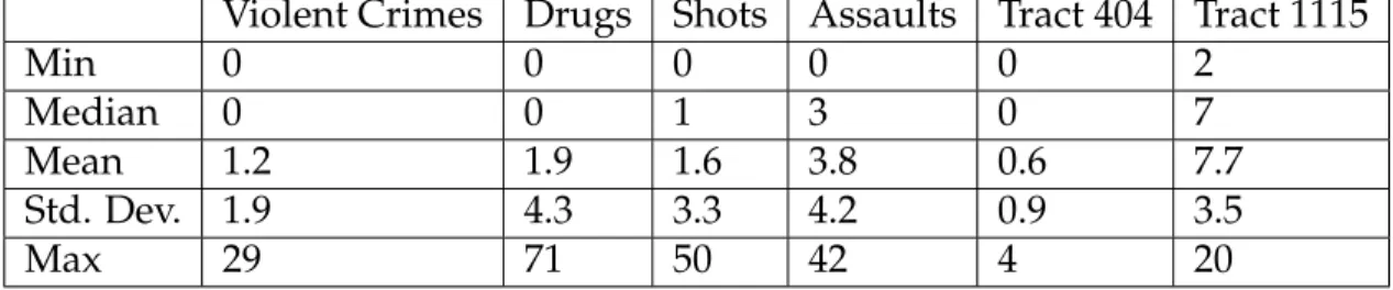
The data used in this paper are monthly crime counts by census tract from Pittsburgh, Pennsylvania. The dependent variable is the count of serious vio-lent crimes (homicide, rape, robbery, and aggravated assault) while the 12 lead-ing indicators are one, two, three, and four month time lags of illicit drug 911 calls for service, shots-fired 911 calls for service, and offense reports of simple
December 2001 across 175 census tracts with 24,500 observations available out of 25,200 after dropping the beginning four month’s observations used for time-lagged variables. For notation, we defineyas the vector of violent crimes and X as the 12 column matrix of leading indicators. Table 2.1 shows the summary statistics for our data. Tract 404 represents a randomly selected low-crime area while tract 1115 is a random high-crime area. Besides overall performance of the computational experiment, we report forecast performance and gold-standard points for these two arbitrarily-chosen areas in the results section. Note that all crime counts are relatively low for monthly crime time series by census tract in Pittsburgh, making it challenging to obtain high forecast accuracy of any kind.
Violent Crimes Drugs Shots Assaults Tract 404 Tract 1115
Min 0 0 0 0 0 2
Median 0 0 1 3 0 7
Mean 1.2 1.9 1.6 3.8 0.6 7.7
Std. Dev. 1.9 4.3 3.3 4.2 0.9 3.5
Max 29 71 50 42 4 20
Table 2.1: Summary Statistics of Crime Data
2.4.2
Gold Standard Policy
We employed a standardization procedure to define gold standard large changes in violent crimes (chosen to be about three percent of all census tracts) in accordance with Gorr (2009). In each census tract, the number of violent crimes were standardized according to their past smoothed mean and variance to account for the sizable time trends in the multiple-year data. The top five standardized values across all census tracts were labeled large changes each month as a gold standard policy defining positives.
In more detail, we perform a standardization procedure on each time series (i.e., census tract) which shifts and rescales the current actual value in timet,yt
by its smoothed mean mt and variancevt, respectively. A low smoothing
con-stant was used to allow the estimated mean to drift with the time series, but not to change appreciably from month to month. Smoothed means tend to yield data not over dispersed so that the Poisson assumption is valid. Thus we ini-tialize values and assumemt=vtfrom a Poisson distribution assumption since
the number of violent crimes follows a count distribution. For each time pe-riod, we set our standardized value y∗t = yt−√mt
vt and updated the estimates of the smoothed mean and variance by the current actual value. Once all values in each time series are standardized, we select the five largest values (three per-cent) for each month’s cross-section of census tracts to define large increases in crime.
2.4.3
Rolling Horizons
Crime forecasting for deployment of police resources needs only one-step-ahead forecasts (one-month- one-step-ahead in this case). Urban police resources are highly mobile and easily and commonly reassigned or targeted. Also, most modern urban police departments have monthly review and planning meetings by sub- region (zone or precinct) so that one-month-ahead forecasts are needed. While forecasting large decreases in crime is perhaps useful for pulling police resources away from areas, the primary interest is crime prevention and fore-casting large increases. A separate study, of the same magnitude and effort for large decreases, would be necessary for large decreases but is not conducted in
setting has at least moderate success (e