Graph-based Model-Selection Framework for
Large Ensembles
Krisztian Buza, Alexandros Nanopoulos and Lars Schmidt-Thieme Information Systems and Machine Learning Lab (ISMLL) Samelsonplatz 1, University of Hildesheim, D-31141 Hildesheim, Germany
{buza,nanopoulos,schmidt-thieme}@ismll.de
Abstract. The intuition behind ensembles is that different prediciton models compensate each other’s errors if one combines them in an appro-priate way. In case of large ensembles a lot of different prediction models are available. However, many of them may share similar error character-istics, which highly depress the compensation effect. Thus the selection of an appropriate subset of models is crucial. In this paper, we address this problem. As major contribution, for the case if a large number of mod-els is present, we propose a graph-based framework for model selection while paying special attention to the interaction effect of models. In this framework, we introduce four ensemble techniques and compare them to the state-of-the-art in experiments on publicly available real-world data. Keywords.Ensemble, model selection
1
Introduction
For complex prediction problems the number of models used in an ensemble may have to be large (several hundreds). If many models are available for a task, they often deliver different predictions. Due to the variety of prediction models (SVMs, neural networks, decision trees, Bayesian models, etc.) and the differences in the underlying principles and techniques, one expects diverse error characteristics for the distinct models. Ensembles, also called blending or com-mittee of experts, assumes that different models can compensate each other’s errors and thus their right combination outperforms each individual model [3].
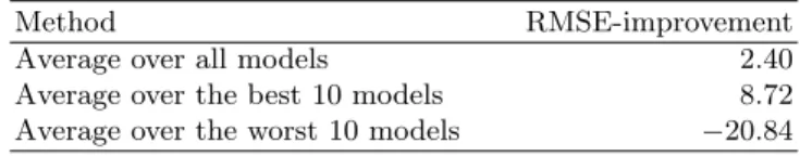
The aforementioned statement can be justified with the simple observation, that the average of the predictions of the models may outperform the best in-dividual model. This is illustrated with an example in Tab. 1, which presents results of simple ensembles of 200 models contained in the AusDM-S dataset.1 Combining all classifiers, however, may not be the best choice: many of the models may share similar error characteristics, that can highly depress the com-pensation effect. In particular, the average of the 10 individually best models’ predictions outperforms the average of all the predictions. (See Table 1.) Instead, if one selects the 10 individually worst models, the average of their predictions perform much worse than the best model.
1
Table 1.Performance (Root Mean Squared Error) improvement w.r.t. best individual model using simple ensemble schemes on the AusDM-S dataset. (10 fold cross valida-tion, averaged results, in each fold the best/worst model(s) were selected based on the performances on the train subset.)
Method RMSE-improvement
Average over all models 2.40
Average over the best 10 models 8.72 Average over the worst 10 models −20.84
We argue that different models have a high potential to compensate each other’s errors, but the right selection of the models is important otherwise this compensation effect may be depressed. How much the compensation effect is depressed, also depends on how robust is the applied ensemble schema against overfitting. In case of well-regularized ensemble methods (like stacking with lin-ear regression or SVMs) the depression of compensation is typically much lower. E.g. training a multivariate linear regression as meta-model onall predictions of AusDM-S is still worse than training it on the predictions of theindividually best 10 models(RMSE-improvement: 8.58 vs. 9.42). Note, however that the selection of the 10 individually best models may be far from perfect: the potential power of an ensemble may be much higher than the quality we reach by combining the 10 individually best models. Thus, even in case of well-regularized models, the depression of compensation is an acute problem.
In this paper, we address this problem. As major contribution, we propose a new graph-based framework that is generic enough to describe a wide range of model selection strategies for ensembles varying from filter to meta-wrapper methods.2 In this framework, one can simply deploy our ensemble method, that successfully participated in the recent Ensembling Challenge at the Australian Data Mining Conference 2009. Using the framework, we propose 4 ensemble techniques: Basic, EarlyStop, RegOpt and GraphOpt. We evaluate these strategies in experiments on publicly available real-world data.
2
Related Work
Ensembles are frequently used to improve predictive models, see e.g. [8], [7], [6]. The theoretical background, especially some fundamental reasons, why ensem-bles work better than single models were discussed in [3].
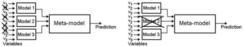
Our focus in this paper is on a generic framework in order to describemodel selection strategies. Such an approach can be based on the stacking schema [9] (also called stacked generalization[12]), in context of which, model selection is feature selection at the meta-level (and variable selection is feature selection at the elementary level), see Fig. 1. In the studied context, related work includes feature selection at the elementary level [5] [4]. Some more closely related works
2
Fig. 1.Feature selection in ensembles: at the elementary level (variable selection, left) and at the meta-level (model selection, right).
Algorithm 1Edge Score Function: edge score
Require: Modelmj, Modelmk, data sampleD, ErrorFunctioncalc err
Ensure: Edge weight of{mj, mk}
1: p1=mj.predict(D),p2=mk.predict(D),∀x:p[x] = (p1[x] +p2[x])/2
2: return calc err(p,D.labels)
study feature selection at the meta level, e.g. Bryll et al.[2] applies a ranking of models and selects the best models to participate in the ensemble. In our study, for comparison purposes, we use the schema of selecting the best models as baseline to evaluate our proposed approach.
Other, less closely related work includes Zhou et al.[14], who employed a genetic algorithm to find meta-level weights and selected models based on these weights. They found, that the ensemble of the selected models outperformed the ensemble of all of the models. Yang et al. [13] compared model selection and model weighting strategies for Ensembles of Naive-Bayes-extensions, called “Super-Parent-One-Dependence Estimators” (SPODE) [11]. All of these works focus on specific models: Zhou et al.[14] are concerned with neural networks, whereas Yang et al. focused on SPODE Ensembles[13]. In contrast to them, we develop a general framework, that operate with various models and meta-models. The model selection approach by Tsymbal et al.[10] is also essentially different from ours: they select (dynamically) those models that deliver the best predictions individually. In contrast, we view the task more globally by taking interactions of models into account and thus supporting less-greedy strategies. Bacauskiene et al. [1] applied genetic algorithm for finding the ensemble settings both at the elementary level (hyper-parameters and variable selection) and at the meta-level. However, due to their high computational cost, genetic algorithms are impractical in our case of having large number of models present.
3
Graph-based Ensemble Framework
Given the prediction modelsm1, . . . , mN, our goal is to find their best
com-bination. As mentioned before, the key of our ensemble technique is the selection of models that compensate each other’s errors. For this, we build a graph first, the model-pair graph, denoted as g in Alg. 2 (line 5). Each vertex corresponds to one of the modelsm1, . . . , mN. The graph is complete (all vertices are
Algorithm 2Graph-based Ensemble Framework
Require: SubsetScoreFunctionf, Predicateexamine, ErrorFunctioncalc err, ModelTypemeta model type, Intn, Real, set of all modelsMSet, labelled dataD Ensure: Ensemble of selected models
1: data[ ]splits = splitDinto 10 partitions 2: fori= 0;i <10;i+ +do
3: dataDA←splits[i]∪. . .∪splits[ (i+ 4) mod 10 ]
4: dataDB ←splits[ (i+ 5) mod 10 ]∪. . .∪splits[ (i+ 9) mod 10 ]
5: g←build graph with edge scores calculated by Alg. 1 for all edges{mj, mk }
6: Mi← ∅
7: Let scoreMi be the worst possible score
8: E(g)←sort the edges ofgaccording to their weights, begin with the best one 9: for alledge{mj, mk}inE(g), process edges according to the orderdo
10: if (mj∈Mi∧mk∈Mi thenproceed for the next edge
11: if examine({mj, mk}) then 12: Mi0←Mi∪ {mj} ∪ {mk} 13: scoreMi0←f(M 0 i, DA, DB,calc err, g) 14: if scoreM0
i better thanscoreMi at least bythen
15: Mi←Mi0, scoreMi←scoreM0 i 16: end if 17: end if 18: end for 19: end for
20: Mf inal← {m∈M Set|mis included in at leastnsets amongM0. . . M9}
21: M ← train a model of type meta model type over the prediction vectors of the models inMf inalusingD
22: return M
reflects the mutual error compensation power ofmj andmk. In Alg. 1 for each
data instance, we average thepredicitions of the both regression modelsmj and mk (line 1). This gives a new prediction vectorp. Then the error ofpis returned
(line 2), which is used as the weight of edge{mj, mk}.
Alg. 2 shows the pseudocode of our ensemble framework. This works with variouserror functions,subset score functionsandmeta model types. The method iterates over the edges of the graph (lines 9. . . 18). To scale up the selection, one can specify a predicate called examine that determines which edges should be examined and which ones should be excluded. As we will see in section 4, the specific choice of these parameters result in various ensemble methods having the common characteristic, that they all exploit the error compensation effect.
While learning, we divide the train data into two disjoint subsets DA and DB (lines 3 and 4)3and we build the model-pair graph (line 5). The division of
the train data is iteratively repeated in a round robin fashion (see line 2). We process the edges in order of their scores, beginning with the edge which corresponds to the best pair of models, see lines 6. . . 18. (E.g. in case of RMSE
3
This is a natural way to split because it allows effective learning of the selection since it balances well between fitting and avoiding of overfitting.
smaller values indicate better predictions, so we process the edges inascending
order with respect to their weights.)Midenotes a set of models, that are selected
in the i-th iteration, scoreMi denotes the score of Mi. This score reflects how
good is the ensemble based on the models inMi. When iterating over the edges
of the model-pair graph, we try to improvescoreMi by adding models toMi.
In each iteration we select a set of models Mi. Mf inal denotes the set of
such models that are contained at leastntimes among the selected models, i.e. improve at least n times by at least . Finally, we train a model M of type
meta model type over the output of models in Mf inal using all training data
instances. ThenMcan be used for the prediction task (for unlabelled data). Note, that our framework operates fully at the meta level: the attributes of data instances are never accessed directly, only the prediction vectors that the models deliver for them. Also note, that the hyperparameters ( andn) can be learned using a hold-out subset of the train data that is disjoint fromD.
4
Ensemble Techniques
As we mentioned, the specific choice of the i) error function calc err, ii) subset score function f, iii)examine predicate and iv)meta model type lead to differ-ent ensemble techniques. In all of our techniques the error function calculates RMSE (root mean squared error). As meta model type we chose multivariate linear regression. In the followings, we describe further characteristic settings of our ensemble techniques.
Basic When searching for the appropriate subset of models Mi, we calculate
thecomponent-wise average of prediction vectorsof models inMi and based
on that we score that subset of modelsMi. We use favg (Alg. 3) as subset
score function in Alg. 2 at line 13. Theexaminepredicate is constant true. EarlyStop In order to save time we only examine the bestNedges (w.r.t. their
weights) of the model-pair graph. For this we useexaminetopNpredicate that
is true for the bestN edges of the model-pair graph and false else. As subset score function, similar to the Basic technique, we chosefavg.
RegOpt Like in EarlyStop, we use theexaminetopNpredicate. However, instead
offavg we use multivariate linear regression to score the current model
se-lection in each iteration (seefreg in Alg. 4).
GraphOpt This operates exclusively on the model-pair graph: we chose the
fgoptsubset score function (Alg. 5) and theexaminetopNpredicate. Function
fgoptcalculates an average-like aggregation of the edge weights, but it gives
priority to larger sets, as the sum of the weights is divided by a number that is larger than the number of edges (as we use RMSE as error measure, smaller numbers correspond better scores). If simply the average were calculated (without priorising large sets), the set M containing solely the vertices of the best edge (and no other vertices) would maximize the score function and that would not be capable to find model set having larger size than 2.
Algorithm 3Score Average Prediction:favg
Require: ModelsetM, Data samplesDA andDB, ErrorFunctioncalc err, Graphg
1: for∀mi∈M dopi=mi.predict(DB),
2: ∀x:p[x] = (p1[x] +. . .+pi[x] +. . .)/M.size (predictions averagedperinstance)
3: return calc err(p,DB.labels)
Algorithm 4Score Model Set using Linear Regression:freg
Require: ModelsetM, Data samplesDA andDB, ErrorFunctioncalc err, Graphg
1: for∀mi∈M dopAi =mi.predict(DA),
2: for∀mi∈M dopBi =mi.predict(DB),
3: Train multivariate linear regressionLusingpA
i as data andDA.labels as labels
4: p=L.predict(pBi)
5: return calc err(p,DB.labels)
Basic examinesO(N2) edges (N is the number of models). Asexamine topN
returns true for the most promising edges, we expect that EarlyStop does not lose much on quality against Basic, but the runtime is reduced by an order of magnitude, as EarlyStop examines only O(N) edges. We expect RegOpt to be slower than EarlyStop, because from the computational point of view, training a linear regression is more expensive then calculating an average. On the other hand, as freg is more sophisticated thanfavg, we expect quality improvement.
RegOpt works in a meta-wrapper fashion, but filter methods, like GraphOpt, are expected to be faster, as they do not invoke the meta-model in the phase of model selection. Nevertheless, GraphOpt may produce worse results as only the information encoded in the model-pair graph is taken into account.
Note, that we expect well-performing ensemble techniques, if the score func-tionf and themeta model type are chosen in a way that there is a natural cor-respondence between them, like in case of our ensemble techniques. Also note, that Alg. 3 and 4 are conceptual descriptions of the score functions: in the imple-mentation, the base models are not invoked as many times as the score function is called, but their prediction vectors are pre-computed and stored in an array.
5
Evaluation
Datasets.We used the labelled datasets, namelySmall(AusDM-S, 200 models, 15000 cases),Medium(AusDM-M, 250 models, 20000 cases) andLarge (AusDM-L, 1151 models, 50000 cases) of the RMSE task of the Ensembling Challenge at the Australian Data Mining Conference 2009. These data sets are publicly avail-able at http://www.tiberius.biz/ausdm09/. They contain the outputs of differ-ent prediction models for the same task, movie rating prediction. The prediction models were originally developed by different teams of the Netflix challenge. There the task was to predict how users rate movies on a 1 to 5 integer scale (5=best, 1=worst). In AusDM, however, both the predicted ratings and the target were multiplied by 1000 and rounded to an integer value.
Algorithm 5Score Model Set using the Model-Pair Graph:fgopt
Require: ModelsetM, Data samplesDA andDB, ErrorFunctioncalc err, Graphg
1: SumW←0
2: for(∀{mi, mj}|mi, mj∈M) do SumW←SumW +g.edgeWeight({mi, mj})
3: return SumW (M.size)2∗ln(M.size)
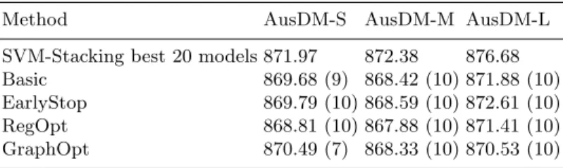
Table 2. Performance of the baseline and our methods: root mean squared error (RMSE) on test data averaged over 10 folds. The numbers in parenthesis indicate in how many folds our method won against the baseline.
Method AusDM-S AusDM-M AusDM-L
SVM-Stacking best 20 models 871.97 872.38 876.68 Basic 869.68 (9) 868.42 (10) 871.88 (10) EarlyStop 869.79 (10) 868.59 (10) 872.61 (10) RegOpt 868.81 (10) 867.88 (10) 871.41 (10) GraphOpt 870.49 (7) 868.33 (10) 870.53 (10)
Experimental settings. We have examined several baselines, namely Tsym-bal’s method[10], as well as stacking of different number of best models with LinearRegression and SVM (this selection of the individually best models is in accordance with [2]). To keep comparison clear, we select as single baseline, the stacking of the individually best models with SVMs, because SVM is generally regarded as one of the best performing regression/classification methods.4 We used the WEKA-implementations (http://www.cs.waikato.ac.nz/˜ml/) of SVM (for the baseline) and Linear Regression (for RegOpt). We performed 10-fold-crossvalidation.5 The hyperparameters of the SVM and our models (complexity
constant C, exponent of the polynomial kernel e; and n, respectively) were searched on a hold-out subset of the train data.6
Results.The results on test data are summarized in Tab. 2. Similarly to [11] and [13], we report the number of folds where our method won against the baselines. Discussion. All of our proposed techniques clearly (in the majority of folds) outperform the baselines. As expected, compared toBasic,EarlyStoplost almost nothing in terms of quality. RegOpt however outperformed not only EarlyStop
but Basic as well. GraphOpt, that works according to the filter schema, could
4 In our reported results, we used stacking of the 20 individually best models. The
reason is two-fold: i) this number leads to very good performance for the baseline, and ii) ensures fair comparison of all examined methods by making them have ap-proximately the same number of selected models.
5
The internal data splitting in Alg. 2 is performed each time only on the current train-ing data of the 10-fold-crossvalidation. In each round of the 10-fold-crossvalidation, Alg. 2 is executed according to which this internal splitting of the current training data is iteratively repeated several times in a round robin fashion.
6
To simplify the reproduciblity, we report the found SVM-hyperparameters:e= 20= 1 andC= 2−5 (AusDM-S),C= 2−3 (AusDM-M),C= 2−8 (AusDM-L).
still outperform the baselines, but it did not clearly outperformBasic. Regarding runtimes, we observedEarlyStop to be 3.3-times faster thanBasic on average, whereasGraphOptwas 1.65-times more performant thanBasic, andRegOptwas 1.4-times faster thanBasic. This is in accordance with our expectations.
6
Conclusion
We proposed a new graph-based ensemble framework that supports stacking-based ensemble with appropriate model selection in the case if large number of models are present. We put special focus on the selection of models that compensate each other’s errors. Our experiments showed that our four techniques implemented in this framework outperforms the state-of-the-art technique. Acknowledgements. This work was co-funded by the EC FP7 project MyMedia under the grant agreement no. 215006. Contact: [email protected].
References
1. M. Bacauskiene, A. Verikas, A. Gelzinis, and D. Valincius. A feature selection technique for generation of classification committees and its application to catego-rization of laryngeal images. Pattern Recognition, 42:645–654, 2009.
2. R. Bryll, R. Gutierrez-Osuna, and F. Quek. Attribute bagging: improving accu-racy of classifier ensembles by using random feature subsets. Pattern Recognition, 36(6):1291–1302, 2003.
3. T. G. Dietterich. Ensemble methods in machine learning. InMCS, volume 1857 ofLNCS, pages 1–15. Springer-Verlag, 2000.
4. Tin Kam Ho. The random subspace method for constructing decision forests.IEEE Trans. Pattern Anal. Mach. Intell., 20(8):832–844, 1998.
5. G.-Z. Li and T.-Y. Liu. Feature selection for bagging of support vector machines. InPRICAI 2006, volume 4099/2006 ofLNCS, pages 271–277. Springer, 2006. 6. Y. Peng. A novel ensemble machine learning for robust microarray data
classifica-tion. Computers in Biology and Medicine, 36(6):553–573, 2006.
7. C. Preisach and L. Schmidt-Thieme. Ensembles of relational classifiers. Knowl. Inf. Syst., 14:249–272, 2008.
8. A.C. Tan and D. Gilbert. Ensemble machine learning on gene expression data for cancer classification, 2003.
9. K. M. Ting and I. H. Witten. Stacked generalization: when does it work? InInt’l. Joint Conf. on Artificial Intelligence, pages 866–871. Morgan Kaufmann, 1997. 10. A. Tsymbal and D.W. Patterson S. Puuronen. Ensemble feature selection with
simple bayesian classification. Inf. Fusion, 4:87–100, 2003.
11. G. I. Webb, J. R. Boughton, and Z. Wang. Not so naive bayes: Aggregating one-dependence estimators. Mach. Learn., 58(1):5–24, 2005.
12. D. H. Wolpert. Stacked generalization. Neural Networks, 5:241–259, 1992. 13. Y. Yang et al. To select or to weigh: A comparative study of linear combination
schemes for superparent-one-dependence estimators. IEEE Trans. on Knowledge and Data Engineering, 19:1652–1665, 2007.
14. Z.-H. Zhou, J. Wu, W. Tang, Zhi hua Zhou, Jianxin Wu, and Wei Tang. Ensembling neural networks: Many could be better than all. Artificial Intelligence, 137(1– 2):239–263, 2002.