by
Nuovella Williams
A thesis
submitted to the Victoria University of Wellington
in fulfilment of the
requirements for the degree of
Doctor of Philosophy
in Statistics.
Victoria University of Wellington
2006
Abstract
The advent of new technology for extracting genetic information from tissue samples has increased the availability of suitable data for finding genes controlling complex traits in plants, animals and humans. Quantitative trait locus (QTL) analysis relies on statistical methods to interpret genetic data in the presence of phenotype data and possibly other factors such as environmental factors. The goal is to both detect the presence of QTL with significant effects on trait value as well as to estimate their locations on the genome relative to those of known markers.
This thesis reviews commonly used statistical techniques for QTL mapping in experimental populations. Regression and likelihood methods are discussed. The mixture-modelling approach to QTL mapping is explored in some detail. This the-sis presents new matrix formulas for exact and convenient calculation of both the Observed and Fisher information matrices in the context of Multinomial mixtures of Univariate Normal distributions. An extension to Composite Interval mapping is proposed, together with a hypothesis testing strategy which is robust enough to de-tect existing QTL in the presence of slight deviations from model assumptions while reducing false detections.
Acknowledgements
This work was funded by a Commonwealth Scholarship from the New Zealand Vice Chancellor’s Committee. I also acknowledge the help of the Training Division of the Government of Montserrat in facilitating access to this research opportunity.
Many thanks to my supervisors Dr. Richard Arnold and Dr. Ross Renner for their help and encouragement throughout this research project. I am also grateful to the administrative and computing staff of the School of Mathematics, Statistics and Computer Science (Victoria University of Wellington) for their support.
VUW, New Zealand Nuovella Williams
Table of Contents
Abstract ii
Acknowledgements iii
Table of Contents iv
List of Tables vii
List of Figures ix
1 Introduction 1
1.1 Successes . . . 5
1.2 Usefulness and Verifiability . . . 6
1.3 The Challenges of QTL Mapping . . . 8
1.4 Review of the model-development literature . . . 12
1.5 Contribution of this Thesis . . . 18
1.6 Thesis Layout . . . 18
2 Linkage, Breeding Designs and Genetic Effects 20 2.1 Linkage and Recombination Fractions . . . 20
2.2 Breeding designs . . . 23
2.3 Genetic effects . . . 27
2.3.1 Additive, dominance and epistatic effects . . . 27
2.3.2 Harmonized definitions of genetic effects . . . 35
2.3.3 Partitioning the genetic variance . . . 37
2.3.4 Number of genetic effects in a full linear regression model . . . 39
3 The Inherent Mixture 41 3.1 Statistical Exploration of Line-Cross data . . . 41
3.2 From marker to QTL . . . 46
4 Regression Methods 53 4.1 Multiple Regression with Contrasts . . . 54
4.1.1 Models, contrasts and implications . . . 54
4.1.2 Sums of Squares and Hypothesis Tests . . . 60
4.1.3 Inferring QTL from marker regression . . . 63
4.1.4 Choice of Contrasts . . . 68
4.2 An example based on single-marker regression . . . 71
5 A Robust Interval Mapping Procedure 77 5.1 The Model Specification for RIM1 . . . 79
5.1.1 Genotypic content of the backcross population at the loci under study . . . 79
5.1.2 Relating genotypic content to trait value . . . 81
5.1.3 The model matrix and likelihood function for a sample . . . . 90
5.2 Maximum Likelihood Analysis . . . 93
5.2.1 Maximization Procedure . . . 93
5.2.2 The conditional observed information matrix . . . 102
5.2.3 The Fisher information matrix . . . 110
5.3 Hypothesis testing . . . 111
5.4 Computational Issues . . . 124
5.4.1 Selecting starting points for the EM Algorithm . . . 124
5.4.2 Stopping rules . . . 129
5.4.3 Adjustments to RIM1 . . . 130
5.4.4 Reduced Models for fitting fewer than three QTL . . . 131
5.4.5 The possibility of a singular information matrix . . . 132
5.4.6 Programming environment . . . 133
6 Information Matrix Derivations 135 6.1 The Complete-Data Conditional Information . . . 136
6.2 Notation and Useful Matrix Identities . . . 138
6.2.1 Notation . . . 138
6.2.2 General Matrix Identities . . . 139
6.2.3 Matrix Identities that are Specific to our Problem . . . 140
6.3 Conditional Expectations of Products of the Estimated Category Iden-tities . . . 144
6.4 Conditional Expectations of Outer Products of the Score Vectors . . . 148
6.6 Intermediate Results Involving Integrals . . . 174
6.7 The Fisher Information Matrix . . . 179
7 Simulations and Results 189 7.1 The Single-QTL Situation . . . 190
7.1.1 Quality of the MLEs of QTL effect and position . . . 197
7.1.2 Performance of the Fisher information matrix . . . 209
7.1.3 Hypothesis testing . . . 220
7.2 The Multi-QTL Situation . . . 226
8 Other Breeding Designs and Real Data Applications 230 8.1 Including interactions between QTL . . . 230
8.2 Application to Other Inbred Designs . . . 231
8.2.1 Application to the F2 . . . 232
8.2.2 Designs involving loci with more than two alleles . . . 235
8.3 Applications to real data . . . 236
8.3.1 Real F2 Application . . . 237
8.3.2 Real Backcross Application . . . 240
8.4 Overview . . . 245
9 Summary and Conclusions 246 A Constructing an Orthogonal Contrast Matrix 251 B Programs and Code 254 B.1 R code for parameter estimation in RIM1 and its sub-models . . . 255
B.2 Utility functions for QTL analysis (R Code) . . . 307
B.3 Examples of using the utility functions with QTL Cartographer . . . 316
B.4 R code to implement the information matrix formulas for RIM1 and its sub-models . . . 322
B.5 Using the RIM1 functions in batch mode - an example . . . 351
B.6 Permutation tests with RIM1 . . . 353 B.7 Using the RIM1 functions with the Horvat and Medrano mouse data 355
List of Tables
3.1 Some population properties of line cross designs . . . 43
3.2 Some sample properties of line cross designs . . . 44
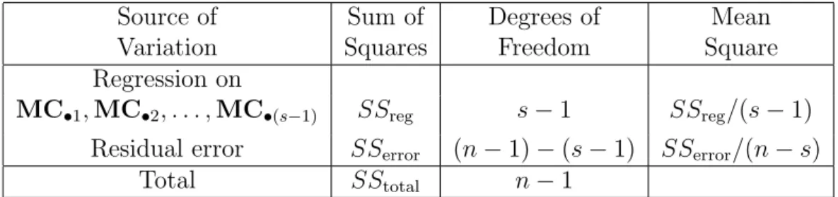
4.1 One-way ANOVA table. . . 62
4.2 Contrasts to extract genotypic effects for a backcross model . . . 69
4.3 Contrasts to extract genotypic effects for an F2 model . . . 70
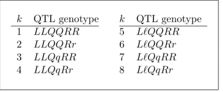
5.1 QTL genotypes and their indices in a B1-backcross model with loci in the order L-M-Q-N-R. . . 80
5.2 Calculation of P(xL|xK, xM) for the B1 Backcross . . . 86
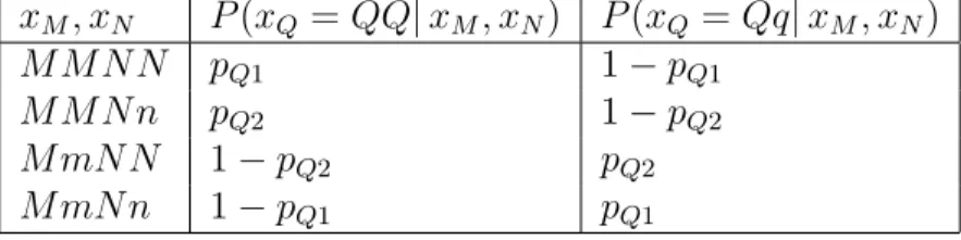
5.3 Calculation of P(xQ|xM, xN) for the B1 Backcross . . . 86
5.4 Calculation of P(xR|xN, xO) for the B1 Backcross . . . 86
5.5 Conditional genotype probabilities, wik, for the B1 Backcross . . . 87
6.1 Selected conditional expectations involving products of estimated cat-egory identities . . . 144
6.2 List of propositions that provide formulae for calculating the condi-tional expectation of the outer product of the score vector . . . 148
6.3 List of integrals used for calculating of the Fisher information matrix. 174 7.1 An Example of raw output from our RIM1 implementation . . . 193
7.2 Summarising the output of RIM1 . . . 196
7.4 Simulated Single-QTL Case: Interval c2m7-c2m8; comparison of
esti-mated standard errors (SD) ofbbQ . . . 210
7.5 Standard error of estimated QTL effect from RIM1 on replicates . . . 211
7.6 Standard error of estimated QTL effect from CIM on replicates . . . 211
7.7 Simulated Single-QTL Case: Interval c2m7-c2m8; comparison of esti-mated standard errors (SD) ofpbQ2 . . . 213
7.8 MLE of QTL location and its estimated standard error from RIM1 on replicates . . . 214
7.9 MLE of QTL location and its estimated standard error from CIM on replicates . . . 215
7.10 RIM1 on bootstraps: standard error of estimated QTL effect. . . 219
7.11 RIM1 on bootstraps: standard error of estimated QTL location. . . . 219
7.12 Percent of times p-value<0.001 for different tests applied to Simulated backcross data; single QTL, sample size 2000 . . . 221
7.13 Percent of times p-value < 0.001 for ten testing methods applied to Simulated backcross data; single QTL, sample sizes 500 and 125 . . . 222
7.14 Multi-QTL case: QTL locations and effects used for simulations. . . . 226
7.15 Percent of times p-value < 0.001 for nine testing methods applied to multi-QTL situation; simulated backcross data . . . 228
8.1 Marginal genotype probabilities in the F2 for three loci . . . 233
8.2 Conditional QTL genotypic probabilities in the F2 . . . 233
8.3 Results of applying RIM1 to a real F2 dataset . . . 239
8.4 Results of applying RIM1 to a real backcross dataset . . . 244
8.5 Results of bootstrapping a real backcross dataset . . . 245
B.1 List of functions used for model fitting . . . 255
B.2 List of utility functions . . . 307
List of Figures
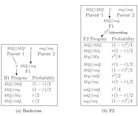
2.1 Definitions of backcross and F2 progeny . . . 25
2.2 Definitions of Second Backcross and Doubled Haploid lines . . . 25
5.1 Model genetic map . . . 79
5.2 Plots of pQ1 versus rM Q and min(pQ2) versusrM N . . . 88
5.3 Plot of pQ2 versus rM Q . . . 89
5.4 Grid for selecting starting values for the EM Algorithm . . . 125
7.1 Single-QTL, genetic map on which simulations were based . . . 191
7.2 Scatter plots of brM Q from CIM based on simulated samples of sizes 125, 500 and 2000 . . . 198
7.3 Scatter plots of brM Q from RIM1 based on simulated samples of sizes 125, 500 and 2000 . . . 200
7.4 Box plots ofbbQ and from CIM and and CIM-QTLcart, based on sim-ulated samples with a single QTL and sample size 2000 . . . 202
7.5 Box plots ofbbQ and pbQ2(1−pbQ2) (bbQ)2 from RIM1 based on simulated samples with a single QTL and sample size 2000 . . . 203
7.6 Box plots illustrating the ability of RIM1 to detect QTL to the left and the right of a testing interval . . . 204
7.7 Box plots of pbQ2(1−pbQ2) (bbQ)2 from CIM and CIM-QTLcart, based on simulated samples with a single QTL and sample size 2000 . . . . 206
7.8 Box plots ofbbQ and pbQ2(1−pbQ2) (bbQ)2 from RIM1 based on simulated samples with a single QTL and sample size 500 . . . 207
7.9 Box plots ofbbQ and pbQ2(1−pbQ2) (bbQ)2 from RIM1 based on simulated samples with a single QTL and sample size 125 . . . 208 7.10 Box plots showing distributions of pbQ2 from RIM1 . . . 214 7.11 Box plots showing distributions of pbQ2 from CIM . . . 215 7.12 Box plots of the estimates pbL2,pbQ2 and pbR2 obtained from RIM1 . . . 216 7.13 Using Permutations to remove a QTL effect . . . 225 7.14 Multi-QTL, genetic map on which simulations were based . . . 227 8.1 Horvat and Medrano mouse map . . . 237
Chapter 1
Introduction
A trait is a quantitative or qualitative characteristic of an individual that is observ-able and that is used to define a phenotype or character of interest. Phenotypes are generally classified according to the type of trait values (discrete/qualitative, con-tinuous/quantitative) used to define them, or according to the mode of inheritance (Mendelian inheritance, complex inheritance) which is hypothesized by the analyst. Gelderman (1975) coined the phrase Quantitative trait locus (or loci) (QTL) to mean a gene (or genes) controlling a quantitative character.
QTL detection techniques use statistical tools to determine if genes significantly affecting the expression of a trait exist within a given search region on a particular chromosome. QTL detection aims to estimate genetic effects and mean trait values within genotype groupings.
QTL mapping goes further, by using more specialized statistical tools to determine approximate QTL positions relative to those of other genes, called markers, whose chromosomal locations are known. QTL mapping estimates the genetic distance between a QTL and a marker. The genetic distance is the number of crossovers or recombinations that occur between the two loci during meiosis, whereas the physical distance between them is the number of nucleotide pairs (base pairs) between the loci.
Genetic distance is measured in Morgans or centiMorgans (cM) , where a Morgan is the distance over which one recombination event is expected to occur per generation, and one centiMorgan is equal to 0.01 Morgans.
The relationship between genetic distance and physical distance can vary at dif-ferent points along a chromosome and it varies from species to species. In humans, 1cM is approximately equal to one million base pairs. QTL analysis is motivated by the need to understand the mechanisms governing one or more quantitative traits, to find the genes involved and to understand their cellular functions.
In studies of agronomically important plants and animals, the traits which cap-tivate the attention of researchers are those which affect productivity. Consider for example, the QTL analysis of soybean seed protein and seed oil by Chunget al.(2003) where the trait-values were assayed using near-infrared reflectance spectroscopy. This method enabled the protein content and seed oil to be quantified by weight (in grams per kilogram of dried meal), so that the values were suitable for quantitative data analysis.
Price et al. (1997) analysed genetic contributions to drought resistance in up-land rice by searching for associations between genetic markers and two shoot-related mechanisms, stomal closure and leaf rolling, which are evident in rice and which re-duce transpirational water loss. They measured stomal closure by using a special instrument called a porometer and then they created three trait assessments from the porometer readings: stomal resistance before excision, time taken after excision to reach the fastest rate of stomal closure, and a score of the rate of stomal closure from one to four (slowest to fastest), based on visual assessment of plots of stomal resistance against time. They measured leaf rolling by the time (in minutes) taken for a young fully-expanded leaf to completely roll up after it was cut from the plant and placed on a flat bench. These traits (along with the corresponding genetic data) were separately analysed in order to search for QTL.
Another example is the QTL mapping study carried out by Spelmanet al.(1999), involving New Zealand dairy cattle. They examined 17 non-production traits includ-ing traits such as adaptability to milkinclud-ing, shed temperament, stature, rump width, rump angle, live weight, udder support, teat placement and the farmer’s overall opin-ion of each cow. The 17 traits were subjectively scored on a 9-point scale, where one and nine represented biological extremes, so we may say that these were pseudo-quantitative values.
In Human genetics and related studies the traits of interest are generally those associated with health and fitness or with disease susceptibility. For example, in or-der to conduct a genome-wide search for QTL unor-derlying asthma, Xu et al. (2001) recorded several traits from individuals in a sample of 533 Chinese families. They studied nine asthma-related phenotypes including forced expiratory volume in one second, airway responsiveness to bronchorestrictors and bronchodilators, serum total immunoglobulin E (IgE), serum-specific immunoglobulin E, eosinophil count in pe-ripheral blood and skin-prick tests to three different allergens. The paper by Xuet al.
(2001) gives very good detail on exactly how each phenotype was measured.
Animal models are often used to study the genetics of some diseases that affect human populations. Animal models (usually mouse models) have the advantage that they allow a researcher to implement controlled environments for trait development. In laboratory mice, traits may be induced by chemicals, by diet, by other environ-mental determinants or by genes.
The use of laboratory animals allows controlled breeding designs to be imple-mented so that an experimenter can limit the amount of genetic variation that occurs within the population. Also, very large sample sizes can often be obtained. Moreover, certain trait assay methods which cannot be applied to human samples can be used when working with animal models. For example, in order to study the genetics of two risk factors (lipoprotein levels and obesity) associated with coronary artery disease,
Warden et al. (1993) used a mouse model. Warden et al. (1993), measured several traits related to obesity, including body weight, body mass index, percent body fat. Some animals were sacrificed and dissected to obtain the weights (in grams) of three intra-abdominal fat pads as additional measures of obesity.
The examples above hint at the variety of traits and trait assessment schemes which are used in genetic association studies. Notice that trait assay can be carried out by methods that are as diverse as the use of precision instrumentation and the use of (sometimes ad hoc) subjective classification. It is not surprising that the chosen trait and its assay method can affect the choice of QTL detection method, the number and type of QTL detected and the ease of QTL detection. Solving the problem of trait assay is a huge challenge for experimenters. The choice of trait evaluation method may depend on the financial resources available, the available technology, the amenability of the species under study to a particular assay method, and may be governed by ethical and practical constraints.
Frankel (1995) gives a good illustration of the importance of trait definition in his discussion of a case where one disease assay criterion allowed the detection of a single QTL, but when a more accurate assay method was developed, two QTL were found. As suggested by Frankel (1995), the best policy is to access several aspects of the phenotype, and to perform QTL analysis using the data from each aspect that has been evaluated.
Some researchers have proposed methods of simultaneously using several traits to search for QTL controlling them all (see Jiang and Zeng, 1995; Corander and Sillanp¨a¨a, 2002). However, the implications of multiple-trait analysis are not well understood and consequently the most popular approaches to QTL mapping use single-trait analysis techniques.
This thesis looks at the statistical methods that are suitable for analysing any
quantitative and that our assumptions about its distribution are reasonably justifiable within the sampled population. The underlying question will be: suppose that we have observed a continuous trait and that it has multiple genetic determinants, then how do we find the genes which control it and how do we separate pooled genetic effects?
1.1
Successes
QTL analysis studies have allowed successful detection of QTL associated with various traits in different species. Consider the QTL analysis studies cited in the previous section. Price et al. (1997) found one QTL for slow leaf rolling on chromosome 1 of the Bala rice variety. They also found two QTL for stomal closure: one located on chromosomes 3 and one located on chromosome 7 of the Bala rice genome. Spelman
et al.(1999) discovered a QTL for stature on bovine chromosome 14 in New Zealand Dairy cattle but no QTL was found to be associated with the other 16 traits that they studied. Chung et al. (2003) detected a QTL for protein yield in soybean. Xu
et al. (2001) found a very significant QTL for Asthma on human chromosome 2 and evidence for six other QTL of lesser effect.
Hundreds of other reported QTL detections may be found in the literature. Some of these results are available in on-line databases. For example, many QTL map-ping results for rats, mice and humans are available from the Rat Genome Database (RGD), Rat Genome Database Web Site, Medical College of Wisconsin, Milwau-kee, Wisconsin. World Wide Web (URL: http://rgd.mcw.edu/). Another example is the Gramene database (http://www.gramene.org, Ware et al. 2002; Jaiswal et al.
1.2
Usefulness and Verifiability
QTL detection results are useful in so much as they can be applied in plant and animal breeding programs and in positional cloning and characterization of genes. All of these applications are relatively costly and are severely hampered when false QTL detections are pursued. False positive error-rates must be kept low so that the apparent successes of QTL mapping may be translated into true successes in the areas of marker assisted selection and genetic characterization. It is not possible to eliminate all false detections because QTL analysis relies on statistical methods, but a desirable QTL detection strategy should at least keep false positives down to the nominal value of the chosen significance level.
The traditional approach to find the physical location of a gene controlling a Mendelian trait is to begin with a known gene product (a protein with a known func-tion), then determine the protein’s amino acid sequence and use it to isolate the gene. This approach is not practical for mapping complex traits because there is usually no information about what proteins could be involved. The aim of positional cloning is to construct a molecular map by using a genetic map as the starting point. There-fore QTL mapping is performed first. Then overlapping segments of DNA are copied from a region which is defined by a confidence interval for the QTL location. Ge-netic procedures such as mutational analysis are applied to authenticate the selected gene locations. For detailed discussions of positional cloning see Arondel et al. 1992; Tanksleyet al. 1995; Vladutu et al.1999; Janderet al. 2002; Morgante and Salamini 2003.
When two or more QTL exist on the same chromosome, methods which assume a single QTL can reveal a false or ‘ghost’ QTL whose map location is different from any of the true QTL locations (Knott and Haley, 1992). This lack of accuracy hinders positional cloning. Several authors have proposed multiple-QTL models (for example
Kao et al., 1999). This thesis also proposes a multiple-QTL model which is robust against ghosting. Genetic maps having good precision will aid also positional cloning because the range of DNA segments to copy and test will then be relatively small.
Since ancient times, plant and animal breeders have found that they could improve the quality of their stocks by selecting individuals having the desirable phenotype to be the parents of the next generation. The paper by Soller and Medjugorac (1999) provides a good overview of how genetic data can be used together with phenotype data to enhance breeding programs. The paper by Soller and Medjugorac (1999) also describes how the work of early pioneers like Sewall Wright, Sir Ronald Fisher and Jay Lush contributed to developing a framework for applying QTL analysis in breeding programs. Marker assisted selection (MAS) is meant to fine-tune selective breeding schemes by using both phenotypic and genetic characteristics to select parents.
Marker assisted selection exploits the fact that a trait controlling QTL can be indirectly selected by selecting for genotypes of a marker that is located very close to it. Indirect selection is made possible by the fact that tightly linked genes (genes located very close together on the same chromosome) tend to be transmitted together in generations. The aim is to increase the frequency of the desired QTL alleles from generation to generation. If linked QTL can be detected close to known markers, then breeders have an indication of which markers will be useful for MAS. Marker assisted selection depends on QTL analysis results. However, MAS has the advantage that the exact location of the QTL does not need to be estimated. Despite this advantage, there has been very limited success in MAS breeding programs. For example, Milhal-jevicet al.(2004) noted that in most published experiments on MAS only about half of the QTL under selection actually contributed to the realized selection response.
The poor performance of MAS and other applications of QTL mapping output have caused researchers to be very cautious when interpreting and using QTL analysis results. Consequently, the strategies of independent validation and cross validation
(see Visscher et al., 2000; Bohn et al., 2001) and Meta Analyses (see Goffinet and Gerber, 2000; Xu, 2003), have been used to assess uncertainty in QTL mapping. Still, there are many cases where researchers conducting independent experiments have found agreement on the existence and locations of certain QTL. Therefore QTL analysis remains a popular research area because it can allow the detection of genes having large effects and because it has the potential to detect QTL of moderate to small effects, provided that strategies for reducing the uncertainties which plague the data analysis are found. Developing robust QTL analysis techniques is also a worthy endeavour because it provides a means to more effectively use the vast amount of genetic marker data that is being made available through recent genetic mapping projects.
1.3
The Challenges of QTL Mapping
Some of the challenges that affect model development in the context of QTL analysis are described below.
1. There is uncertainty about how QTL genotypes contribute to trait expression. Consequently, there is uncertainty about the conditional distribution of the trait given a particular QTL genotype. The most common approach is to assume that a trait is Normally distributed within samples of individuals who have the same genotype at the selected loci and who come from similar environments.
2. The QTL locations are unknown and QTL genotypes cannot be observed. Therefore the trait distribution conditional on a QTL genotype must be found by applying the theorem of conditional probability with assumptions about the probability of each QTL genotype given each marker genotype.
3. In order to detect association between marker and QTL, the chosen experi-mental design must capture information about the probability of each QTL genotype given each marker genotype. In order to map QTL, it must capture information for linkage. To detect recombination between two loci, the parent under consideration must be heterozygous at both loci. The QTL genotypes in all parents are unknown, therefore a suitable experimental design must allow inferences to be made about the parental QTL genotypes given their observed marker genotypes. This is necessary to allow assessments to be made about the probability that a particular offspring is the result of recombinations between parental marker and QTL loci. Parents from crosses of inbred lines divergent in trait values as well as in their marker genotypes are often used with plant and some animal species. For species in which inbreeding is not feasible, family stud-ies must be used in order to detect recombination. Still, there is uncertainty about the probabilities of different QTL genotypes within the marker-classes generated by any chosen sampling design.
4. Most complex traits are conditioned by more than one locus and there is uncer-tainty about the number of loci involved. The most common approach to this problem is to assume a fixed number of loci. However, models which assume a single QTL often suffer from ghosting (false detections), while models which assume multiple QTL often suffer from identifiability problems. Otto and Jones (2000) discuss some of the limitations of techniques that attempt to estimate the true number of QTL controlling a trait. Where multiple QTL exist, there may also be a need to separate the effects of different QTL.
5. Traditionally, the main emphasis has been on estimating non-interaction terms in a linear model for QTL effects. Specific contrasts of conditional trait means, called additive and dominance genetic effects, receive much attention in the
literature because they have convenient interpretations (Falconer and Mackay (1996)). However, in fitting a linear model, the precise choice of contrasts is not particularly important except for removing the singularity of the model matrix. Any suitable contrasts may be used, and after fitting, any other desired contrasts may then be obtained from the fitted means provided that the number of simultaneous contrasts is not greater than the rank of the model matrix. It is also noteworthy that common breeding designs produce rank-deficient systems. For example, Backcross designs produce rank-deficient systems that do not allow additive and dominance effects to be separated.
6. There is a possibility that interactions may exist between loci. The number of interactions is unknown.
7. QTL expression can also be influenced by non-genetic factors. There are often problems distinguishing genetic effects from environmental effects and evaluat-ing interactions between genetic and non-genetic factors.
8. The heritability of a trait will also affect the power of QTL detection. Heri-tability is a measure of how much of the total trait variation is due to a genetic component. Genes controlling traits with low heritability may be difficult to detect via marker-trait association because most of the variability seen will tend to be absorbed into the random error.
9. Often, estimated QTL effects are confounded with functions of QTL genotype probabilities (which are functions of recombination fractions). This confounding creates bias in the estimated QTL effects. If a QTL is located extremely close to a marker the magnitude of the estimated effect will be biased downwards and so the QTL will be difficult to detect. If a QTL coincides with a marker, then it may go undetected when models assume that markers have no effect on
trait value (the neutral marker assumption).
10. A dense map of markers can improve the accuracy and precision of QTL map-ping but there is a point where adding more tightly linked markers does not add any more information. Fitting a regression based upon very dense marker-map requires large sample sizes to compensate for the degrees of freedom needed to estimate the large number of parameters generated. Depending on the species and the trait being studied, obtaining very large sample sizes may not be possi-ble. The fact that genotypes at linked markers do not segregate independently may reduce the utility of overly dense marker-maps. The explanatory variables may be highly correlated when genotypes of tightly linked markers are used in regression models. If the map is too dense the resulting model matrix is likely to be ill-conditioned, leading to poor parameter estimates and more false QTL detections. If background markers are too close to the position being tested then they can absorb the QTL effects due the high correlation between marker and QTL genotypes. Davarsi and Soller (1994) modelled the cost of raising indi-viduals and scoring markers (for use in a marker-QTL experiment) as a function of marker spacing and the number of scored individuals in order to access how these factors affected the ability to detect QTL. They found that a marker spac-ing between 20 to 30 centiMorgans (cM) generally tends to be optimal and that any marker spacing below 10 cM is generally not cost effective.
11. The quality of QTL mapping results is affected by sample size. If the sample size is too small some genotypes may not be observed or the counts in some genotype classes may be too small to provide reliable estimates of recombination fractions. There are two sample size problems in QTL mapping. The first problem is that biological, ethical and budgetary constraints can make it difficult to obtain large sample sizes. This problem becomes compounded when the trait
of interest is rare. Several factors can affect whether a particular sample size is adequate. These factors include, but are not limited to, the breeding design, marker density, the number and location of QTL, the size of QTL effects and the heritability of the trait, and the data analysis and estimation techniques used. The second problem is that there is currently no established procedure for combining these factors to form criteria for calculating what sample size is large enough to yield reliable QTL mapping results (Frankel, 1995; Belknap, 1998).
1.4
Review of the model-development literature
Tests for differences between conditional means, analysis of variance, linear regression, generalized linear regression, mixed models, likelihood methods, empirical methods, nonparametric methods and Bayesian methods have all been used to analyse quanti-tative trait loci. Many of these methods have been in existence for decades but the availability of high speed computers has opened up new ways of using them. The most widely used models are those based on extensions of the Fisher (1918) linear model.Single marker methods test for association between the trait and the genotypes at each marker, independently, not considering genotypes at any other marker. Single marker analysis may be based on t-tests for differences between means, simple regres-sion or one-way analysis of variance (Solleret al., 1976; Stuberet al., 1987; Edwards, 1987) and likelihood ratio tests (Weller, 1986).
Kearse and Hyne (1994) suggested a generalized least-squares regression approach which uses all markers on a chromosome to improve the precision of single-marker analysis. The differences in mean trait value of the genotypes at each marker locus form the vector of response variables. The vector of explanatory variables comprises
the distance between each marker and a putative QTL. The analysis is repeated for a series of QTL locations along a chromosome. This procedure is also called ‘multipoint mapping’. Critical values are based on the assumption of a chi-square distribution for the residual sum of squares.
Thoday (1961) was among the first to use a pair of adjacent markers to estimate QTL effects and position. The process of detecting a QTL by simultaneously condi-tioning on a pair of markers lying on either side of it later became known as Interval Mapping. Lander and Botstein (1989) proposed a likelihood-based approach to inter-val mapping which assumed an underlying Normal trait distribution for individuals having the same QTL genotype. Like Thoday, Lander and Botstein modelled QTL effects by conditioning on the genotypes at a pair of adjacent markers. However, the latter used maximum likelihood estimation via the EM algorithm (see Dempster
et al., 1977) to estimate QTL effects.
In an attempt to reduce the computational burden of maximum likelihood esti-mation for interval mapping, Bridges and Knapp (1990), Haley and Knott (1992) and Marinez and Curnow (1992) advocated the use of regression methods. They pro-posed carrying out regressions at several putative QTL locations and taking regres-sion estimators at the location that maximizes the regresregres-sion correlation coefficient as approximations to the desired maximum likelihood estimators.
Whittaker et al.(1996) used contrasts of trait means within marker groupings to show that the location and effect of an isolated QTL (having no additional QTL in adjacent intervals) can be estimated from a regression of phenotype on marker type, without the need for numerical search procedures.
The interval mapping approach of Lander and Botstein (1989) and its regression approximations all assume that either there is a single QTL between the markers under consideration, or that there is no QTL anywhere. This leads to a single Normal distribution under the null hypothesis and a Normal Mixture under the alternative
hypothesis. The likelihood ratio test in this situation amounts to a test of departure from normality of the trait distribution. If a single QTL exists within the specified interval, then additional linked QTL will increase the number of mixing components and will contribute to the sampling variance. Additional QTL can also lead to pooling of effects causing biased estimates. If there is no QTL within the specified interval, the presence of linked QTL outside the testing interval will lead to a null distribution which is a normal mixture rather than a single normal distribution. This could lead to false detections if departure from normality of the trait distribution is taken, on its own, to indicate the presence of a QTL. The removal of outliers may be undesirable if the true distribution is a mixture because outliers may result from rare combinations of genotypes which are in fact valid for the mixture. Similarly, transformations to normality may not be desirable if the underlying distribution is in fact a normal mixture. Such transformations could hamper the detection of an existing QTL.
Realizing that the likelihood ratio test (LRT) for normality of the trait distribution does not necessarily constitute a test for a QTL within a specified interval, researchers needed methods for assessing the results of interval mapping in terms of whether a QTL was detected.
Bootstrap and permutation methods are useful where an estimator of a statistical property of interest is available but its distribution is unknown. Churchill and Doerge (1994) proposed an empirical method for calculating approximate significance thresh-olds (critical values) against which to compare test statistics for QTL mapping. They proposed that critical values should be derived from Monte Carlo tests based on the empirical distribution of these statistics. The idea was to draw samples that would be representative of the null hypothesis of no QTL within a selected marker interval. Churchill and Doerge (1994) showed that such a sample can be obtained by randomly assigning an observed trait value, without replacement, to each sampled individual
while leaving its genotype unchanged. Although Churchill and Doerge (1994) men-tion the possibility of extending the permutamen-tion tests to the problem of detecting multiple QTL, this was not explored. In a similar vein, Visscher et al. (1996b) sug-gested using the bootstrap methodology of Efron (1979), with critical values based on the empirical bootstrap distribution of the test statistic. Despite their heavy com-putational requirements, these resampling methods are widely used because they are simple to implement.
Other researchers used semi-parametric and non-parametric methods to allow for the fact that a null distribution could be non-normal. For example, Kruglyak and Lan-der (1995) proposed some Wilcoxon rank-based tests of genetic effects. Zou (2001) considered a single-QTL framework and applied the Kruglyak and Lander (1995) rank based test to estimate quantitative trait effects. However her simulation results showed that for both normal and non-normal data, the non-parametric test performed similarly to the Normal regressions of Haley and Knott (1992). Zou (2001) also pro-posed a semi-parametric approach to interval mapping, based upon the exponential tilt model of Anderson (1979). The exponential tilt model was found to be suscep-tible to identifiability problems similar to those that plague parameter estimation in normal mixtures.
A simple procedure that has proved to be very robust against false detection (ghosting) involves carrying out standard interval mapping with flanking markers to absorb the variance of background QTL. This procedure, called Composite Interval Mapping (CIM), was independently proposed by Rodolphe and Lefort (1993), Zeng (1993, 1994), and Jansen and Stam (1994). These authors showed that CIM can aid the separation of pooled QTL effects provided that Haldane’s map function holds reasonably well, and provided that no extra QTL lie within the intervals bracketed by the nearest flanking markers. However, if Haldane’s map function holds and extra QTL exist within intervals adjacent to the testing interval, then CIM cannot separate
the effects of QTL from the resulting region stretching over three adjacent intervals. Therefore, false detection rates of CIM (traditional LRT based on χ2
1 distribution) are well controlled only when the testing interval is isolated.
Zeng (1993, 1994) proposed models that allow for multiple QTLs and Hayes et al.
(1993); Jiang and Zeng (1995) considered the problem of QTL-environment interac-tions.
Obtaining standard errors for estimates of model parameters in CIM and other mixture models has always been a challenge. Bootstrapping has been proposed as a method of addressing this problem in QTL mapping problems (Visscher et al.
(1996b)). In order to obtain asymptotic standard errors of model parameters in QTL mapping, Kao and Zeng (1997) proposed formulae for calculating the conditional observed information matrix. Kao and Zeng (1997) did not provide formulae for calculating the Fisher information because they did not take the expectation of the conditional information matrix. Also, they did not explore the idea of statistical tests for QTL based upon the asymptotic distribution of the maximum likelihood estimators. Instead, they used a LOD score of 1.5 (as suggested by Lander and Botstein, 1989) to determine the threshold value for rejection of the null hypothesis. The element-wise approach used by Kao and Zeng (1997) is not sufficiently general to make evaluation of the information matrix both practical and accessible for any Multinomial mixture of Normals.
Making the information matrix practical to calculate for mixture likelihoods is a problem that has received much attention in the statistical literature. Hill (1963) used a power series expansion to simplify the Fisher information matrix for a mixture of two univariate Normal distributions having equal variances. Behboodian (1972a, 1973) provided numerical methods for evaluating the Fisher information matrix for mixtures of two Normal distributions and for mixtures of two Exponential distributions.
approximated the observed information matrix, in terms of the gradient vector of the log-likelihood function. In a simulation study, they found that, when compared with standard errors obtained by bootstrapping, this approximation tended to overestimate the variance of the parameter estimates. Therefore Basfordet al.(1997) recommended using standard errors based on bootstrap methods rather than using standard errors based on the observed information formulae of McLachlan and Basford (1987).
The development of Markov Chain Monte Carlo (MCMC) methods has facilitated Bayesian estimation for mixture models (Casella and George 1992; Smith and Roberts 1993; Diebolt and Robert 1994; Carlin and Lewis, 1996, pages 60, and 159-197; Richardson and Green 1997). Subsequently, various researchers have applied Bayesian approaches to parameter estimation in QTL mapping (Guo and Thompson, 1992; Satagopan et al., 1996; Satagopan and Yandell, 1996; Hoeschele et al., 1997; Ball, 2001).
The Bayesian approach is appealing because it allows the number of mixing com-ponents (the number of QTL) to be explicitly included as an unknown parameter in the model, and it also allows estimation of marginal posterior probabilities for the parameters. However, non-identifiability problems can arise with the Bayesian approach to finite mixture modelling and the MCMC method can also suffer from convergence issues (Diebolt and Robert, 1994; Robert, 1996).
This thesis does not explore Bayesian methods for QTL mapping, instead it fo-cuses on the problem of improving hypothesis testing for parameters in mixture mod-els under the maximum likelihood framework. The next section outlines the main contribution of this thesis.
1.5
Contribution of this Thesis
This thesis explores and develops mathematical and statistical techniques that are tailored towards extracting a desired type of information from samples of genetic (DNA) data coupled with measurements of a specific trait. The desired information is any that will enable detection of genes associated with the trait, estimation of their genetic effects and, in the presence of linkage, estimation of their genetic location.
The existing strategies for inferring QTL from multiple regressions of trait value on marker genotypes are consolidated and formalized. Improved hypothesis tests for Composite Interval Mapping are proposed.
A new extension to Composite Interval Mapping is developed. The proposed model, named Robust Interval Mapping Version One (RIM1), may be viewed as a more robust extension of CIM. The RIM1 model fits exactly three putative quantita-tive trait loci (QTL) and it uses maximum likelihood estimation to obtain estimates of model parameters. Applications to simulated and real data show that these meth-ods have strong power to detect QTL while dramatically decreasing the rate of false detections.
New, very flexible, matrix formulae are developed, allowing exact and convenient calculation of both the Observed and Fisher information matrices in the context of Multinomial mixtures of Univariate Normal distributions. Standard errors based on these formulae are then used to create tests which reduce false detections in CIM while retaining power to detect QTL.
1.6
Thesis Layout
A brief overview of the literature was presented in this introductory Chapter. In Chapter 2, there is an overview of classical quantitative genetics definitions of genetic effects, linkage and sampling designs. Chapter 3 looks at the mixture structure of
line-cross designs and highlights aspects of that structure which could carry informa-tion for model development and hypothesis testing. Chapter 4 reviews the Normal regression approach to QTL mapping.
Chapter 5 is a long Chapter where new techniques are introduced: information matrix formulae are introduced in Chapter 5 as well as an extension to composite interval mapping, named Robust Interval Mapping Version One (RIM1). Chapter 6 tackles the derivation of the information matrix formulae which were presented, without proof, in Chapter 5. Although the detailed mathematical proofs given in Chapter 6 are rather tedious, the proofs are necessary because they show why the proposed formulae constitute an exact evaluation of the information matrix.
In Chapter 7, the proposed methods are applied to simulated data. Extensions and applications of the proposed methods to some real data are given in Chapter 8. The final chapter (Chapter 9) summarizes the results of this thesis and discusses areas for further research.
Chapter 2
Linkage, Breeding Designs and
Genetic Effects
This chapter presents an overview of classical Quantitative Genetics Definitions. The first section focuses on linkage, recombination probabilities, mapping populations and experimental designs. In the later sections we look at the definitions ofgenetic effects
as well as useful properties resulting from these definitions.
2.1
Linkage and Recombination Fractions
Two genes are said to be linked if they are located on the same chromosome. The proximity of linked genes to each other affects their probability of being transmitted together from parent to offspring. In meiosis (sperm or egg production) homologous (similar) chromosomes may overlap and exchange genetic material. This process is calledrecombination orcrossing-over. Crossover is more likely to occur in the interval between linked genes that are located far apart than between closely linked genes.
The recombination fraction between two loci is the probability that there will be an odd number of crossovers between them. Even numbers of crossover are generally
not considered because they cannot be observed.
Consider a set of chromosomes for which a number of markers have been mapped, and which contain an unknown number of QTL at unknown locations. For inference about the properties of these QTL, we need to determine the probability of each (multi-locus) QTL genotype conditioned on each marker genotype. Assessment of the recombination fraction between pairs of loci enables us to write down expressions for the probability of multi-locus genotypes and expressions for the probability that a QTL allele is transmitted given that certain marker alleles are transmitted.
Consider three linked loci in the order A-B-C and let rAB and rBC be the prob-abilities of recombinations between lociA and B and lociB and C respectively. Let rAC be the recombination fraction between loci A and C. Recombinations in the different intervals may not occur independently (see Ott 1991). For instance, when the loci are closely linked, a recombination in one interval may reduce the likelihood of recombination in an adjacent interval.
In genetics, lack of independence between crossover events in different intervals is called crossover interference orrecombinational interference. Under independence, a double recombination occurs with probability rABrBC. If its true probability is π11 then the coefficient of coincidence is defined as
c= π11 rABrBC
and recombinational interference is measured by 1−c. In the case of complete inter-ferencec= 0. When c= 1 there is no interference. Positive interference results when c <1 and there is negative interference when c >1.
Define
π11=P(recombination in both intervals) =c rABrBC (2.1) π10=P(recombination in interval A−B only) =rAB(1−c rBC) (2.2) π01=P(recombination in interval B−C only) =rBC(1−c rAB) (2.3) π00=P(no recombination in either interval) = 1−rAB−rBC +c rABrBC (2.4) Recombinations between A and C can occur in two ways. Either there is recom-bination in the intervalA−B and no recombination in the intervalB−C or there is no recombination in the intervalA−B and recombination in the intervalB−C. This leads to the general three-locus addition formula for recombination fractions given in Equation (2.5).
rAC =π10+π01 =rAB +rBC −2c rABrBC (2.5) The expected number of recombination events between two loci is called the genetic distance between them and is measured in Morgans. Genetic map functions are used to translate recombination fractions into genetic distances.
The Haldane (1919) map function is the most commonly used genetic mapping function. It assumes that recombination events occur independently of each other (no interference) and that they occur as points of a Poisson process along each chro-mosome. Under Haldane’s assumptions, the number of crossovers between two loci x Morgans apart has a Poisson(x) distribution. Therefore, Haldane’s map function to convert the recombination fraction rAB to a genetic distance is
x=−1
2log(1−2rAB).
Real data does not usually support the idea of constant levels of interference in all intervals along a chromosome. However, for simplicity, most common map functions assume a fixed value for c in the addition formula for recombination fractions. For example, c= 1 for Haldane’s addition formula. By setting c= 2rAB Kosambi (1944)
produced an addition formula that allows for non-constant interference. Detailed descriptions of these and other map functions may be found in Quantitative Genetics texts (see, for example, Ott 1991, pages 14-19 and 120-129; Liu 1997, pages 318-329). For recombination probabilities up to 0.1, most map functions give similar estimates of the map distance (see, for example, Table 10.9 on page 329 of Liu 1997). For, example, when the recombination fraction is less than or equal to 0.1, the Morgan, Haldane, Kosambi, Felsenstein, Carter-Falconer map functions yield approximately the same map distances. Therefore, for very dense maps, the Haldane assumption does not cause too much concern. It is more of a concern when map density is low.
2.2
Breeding designs
In order to detect association between marker and QTL, the chosen breeding design must capture information for linkage. The most common breeding designs allow assessments to be made about recombination probabilities, genotype probabilities and about the probability of putative QTL genotypes given any marker genotype. This section gives a brief overview of some commonly used experimental populations and breeding designs. Here we are considering diploid organisms only.
In the following discussion, the founding parents (first parents) from which inbred designs are created are denoted by P1 and P2 respectively. The P1 and P2 lines are assumed to be homozygous at all loci. Additionally, the alleles at any locus in the P1 line are assumed to be different from the alleles at the same locus in the P2 line. For convenience, we refer to an allele from P1 line as a ‘high’ allele, and we refer to the corresponding allele from P2 line as a ‘low’ allele. We denote high and low alleles, respectively, by uppercase and lowercase Roman letters. We refer to a (single-locus) genotype from the P1 line as a ‘homozygous-high’ genotype and we refer to the corresponding P2 genotype as a ‘homozygous-low’ genotype.
Inbreeding without selection
1. Backcross: B1 or B2
Two diverging, inbred lines (P1, P2) are crossed and the resulting offspring (F1) are back-crossed with the first parental line (P1) to form the B1 backcross or with the second parental line (P2) to form the B2 line (see Figure 2.1(a)). All parents (F1 or P1) or (F1 or P2) are completely informative for linkage. At any single locus, only two distinct genotypes are possible and they occur with equal probability. At any locus only the homozygous-high and the het-erozygous genotypes are possible in the B1 backcross. Likewise, at any locus, only the homozygous-low and the heterozygous genotypes are possible in the B2 backcross. Consequently the genotype probabilities in these backcross pop-ulations do not occur in Hardy-Weinberg proportions (see, for example, Hartl and Clark, 1997). Nevertheless, the backcross design has the advantage that the genotype phase (that is, the sister-chromatid locations of alleles in a multi-locus genotype) of all backcross individuals can be determined.
2. Second filial line: F2 intercross. Two diverging, inbred lines are crossed
to form the F1 line. Then the F1 is ‘selfed’ or made to undergo brother-sister mating to produce the F2 line (see Figure 2.1(b)). This breeding design is also referred to as an F2 intercross or simply an intercross. One advantage of the F2 design is that its genotypes occur in Hardy-Weinberg proportions. However, only the homozygous F2 individuals are informative for linkage (they allow the origin of the parental alleles to be determined so allowing recombinantions to be identified without ambiguity). Consequently, the homozygous F2 individuals they are the only F2 individuals whose genotype phase can be determined.
3. Second backcross line (BC2). A second backcross line is formed by crossing
M Q//M Q × mq//mq Parent 1 Parent 2 × M Q//mq F1 B1 Progeny Probability M Q//M Q (1−r)/2 M Q//mq (1−r)/2 M Q//M q r/2 M Q//mQ r/2 (a) Backcross M Q//M Q × mq//mq Parent 1 Parent 2 M Q//mq F1 ⊗Inbreeding F2 Progeny Probability M Q//M Q (1−r)2/4 M Q//M q r(1−r)/2 M q//M q r2/4 M Q//mQ r(1−r)/2 M Q//mq (1−r)2/2 M q//mQ r2/2 M q//mq r(1−r)/2 mQ//mQ r2/4 mQ//mq r(1−r)/2 mq//mq (1−r)2/4 (b) F2
Figure 2.1: Definitions of backcross (from parent one) and F2 progeny for a single marker locus (M) and a QTL locus (Q) that are r recombination units apart. In the F2 population, there are nine distinct two-locus genotypes – in the F2, the genotype M mQq has two possible phases: M Q//mq and
M q//mQ. M Q//M Q × F2 Progeny Parent 1 BC2 Progeny Probability M Q//M Q (1−r)/2 M Q//mq (1−r)/2 M Q//M q r/2 M Q//mQ r/2
(a) Second Backcross Progeny
M Q//M Q × mq//mq Parent 1 Parent 2 M Q//mq F1 Tissue Culture DHLs Probability M Q//M Q 1/2 mq//mq 1/2
(b) Doubled Haploid Lines
Figure 2.2: Definitions of a Second Backcross and Doubled Haploid Lines for a single marker locus (M) and a QTL locus (Q) that are r recombination units apart.
2.2(a) illustrates the case where the backcross is made with the first parental line.
4. Doubled haploid lines (DHLs). Doubled haploid lines are formed by
chem-ically treating some organisms to cause them to replicate producing identical copies of themselves (see Figure 2.2(b)). This technique is only practical in a few species, for example, Zebrafish and Drosophila.
5. Advanced intercross lines: AIL or F(t). Advanced intercrossed lines are
formed by repeated selfing or brother-sister mating of F1 overt−1 generations. These are created by random mating of F1 individuals followed by random mat-ing in all subsequent lines over t−1 generations to produce F2. Davarsi and Soller (1995) showed that advanced intercross lines generate more recombination events than F2 or Backcross designs. By assuming that crossovers occur inde-pendently in adjacent intervals, Davarsi and Soller (1995) derived the following formula for the recombination fraction in the F(t) in terms of a recombination fraction (r) in the F2 population:
rt=
1−(1−r)t−2(1−2r)
2 .
6. Repeatedly backcrossed line. If the offspring from a backcross are
repeat-edly mated with the original parents for a specified number of generations, then the resulting cross is called a repeatedly backcrossed line.
Inbreeding with selection
1. Recombinant inbred lines (RIL).Recombinant inbred lines are produced by
inbreeding with selection of recombinants. The F2 line is taken through several generations of ‘selfing’, with selection of recombinant individuals for breeding at each stage. This design provides a method for replication of these recombinant
individuals when asexual reproduction is not possible. Recombinant inbred lines have essentially no within-line genetic variance, but the variance between lines is considerable because each RIL represents a different multi-locus genotype.
2. Nearly isogenic lines (NIL). Nearly isogenic lines are formed by repeated
back-crossing with selection followed by at least one generation of ‘selfing’ or sib-mating. A donor parent is crossed with an inbred line to form an F1 line. The F1 line is then backcrossed to the inbred line for several generations. Then the individuals in the final generation are sib-mated or ‘selfed’ to form a nearly isogenic line.
Outbred designs
1. Experiments orchestrated to extract desired information from specific outbred populations are called, collectively, outbred designs. These include sib-pair designs, relative pair designs, family triads and case-control designs.
Certain outbred designs require QTL mapping techniques that are quite different from those used with inbred designs. However, some of the methodology for analysing QTL in outbred designs are extensions of those used with inbred designs (see Lynch and Walsh, 1997, Chapters 16-18). This thesis looks at methodology for detecting QTL in experimental populations, assuming inbred line-cross designs and diploid organisms.
2.3
Genetic effects
2.3.1
Additive, dominance and epistatic effects
In the Quantitative Genetics literature, the value of a trait (or phenotype) is called the phenotypic value. Likewise, the part of the phenotypic value that is attributable
to an individual’s genotype is called the genotypic value. In addition, the expected values of specific contrasts of mean trait-value amongst the genotype classes (within a study population) are called genotypic effects.
Each genotypic effect measures the contribution of a particular source of genetic variation to the expected value of a specific trait given a specific genotype. Both the size and the direction of each genetic effect depend on the distribution of the trait within the study population as well as the population the gene and genotype probabilities.
Fisher (1918) defined additive and dominance effects in a linear model for the expected value of a trait given a single-locus genotype. Fisher also partitioned the trait variance according to genetic and environmental sources, with the genetic varia-tion further partivaria-tioned into additive and dominance components. Cockerham (1954) and Kempthorne (1954) independently extended Fisher’s model to include more than one locus. This section outlines the Cockerham-Kempthorne definitions for additive, dominance and epistatic genetic effects.
Suppose that a single locusM hasvdistinct alleles and denote them byM1, . . . , Mv respectively. Assume diploid organisms. Suppose also, that
P(Mi) is the probability of allele Mi in the population; P(MiMj) is the population probability of genotype MiMj;
P(Mi|MiMj) is the probability of the allele Mi among all alleles belonging to genotype MiMj.
to (2.9) below. P(Mi) = P(MiMi) + 12 X j6=i P(MiMj) (2.6) v X i=1 P(Mi) = 1 (2.7) v X i=1 X j6i P(MiMj) =P(MiMi) + X j6=i P(MiMj) = 1 (2.8) P(Mi|MiMj) = 1 2, if i6=j 1, if i=j (2.9)
Note that the conditional probability, P(Mi|MiMj), is also the probability that an individual with genotype MiMj will transmit allele Mi to an offspring.
Denote the trait value by the random variable y. Also, let E(y|Mi) represent the mean trait-value of individuals having allele Mi at a single locus and let E(y|MiMj) represent the mean trait-value of individuals with genotype MiMj at that locus. We denote mean trait-value (in the population under study) by µ, where
µ=E(y) = v X i0=1 µ P(Mi0Mi0)E(y|Mi0Mi0) + X j6=i0 P(Mi0Mj)E(y|Mi0Mj) ¶ . (2.10)
The additive effect of an allele is the difference between the mean trait-value of individuals having that allele and the population mean trait-value. It may be interpreted as the phenotypic value associated with a gene that is passed on to an offspring (see, for example, Falconer and Mackay, 1996, pages 112-117). The additive
effect of allele Mi is defined as αMi =E(y|Mi)−µ = v X j=1 P(MiMj|Mi)E(y|MiMj)−µ = v X j=1 P(Mi|MiMj)P(MiMj) P(Mi) E(y|MiMj)−µ = P(MiMi) P(Mi) E(y|MiMi) + 1 2 X j6=i P(MiMj) P(Mi) E(y|MiMj)−µ (2.11)
This implies that αMi = ³ 1 P(Mi) −1 ´ P(MiMi)E(y|MiMi) + ³ 1 2P(Mi) −1´ X j6=i P(MiMj)E(y|MiMj) −X i06=i X j6=i P(Mi0Mj)E(y|Mi0Mj). (2.12)
Equation (2.12) is an example of acontrast: a linear combination of conditional trait means.
The additive effect can be estimated using the coefficients from a regression of the trait value on the number of copies of target alleles in the genotype. A direct consequence of the definition of additive allelic effect (as given in Equation (2.11)) is that the mean value of the additive allelic effects at a locus is equal to zero:
v X j=1 P(Mj)αMj = 0 =⇒ αMi =− 1 P(Mi) X j6=i P(Mj)αMj. (2.13)
So far, we have discussed the additive effect of a single allele (the additive allelic effect) at a single marker M. Now we turn to the additive effect of a genotype at locus M. Distinct alleles Mi and Mj of the gene at locus M are called codominant alleles if the alleles can be individually identified in the heterozygous genotype MiMj (i6=j). The ability to distinguish loci, and the ability to identify alleles at those loci,
depends on the instrumentation and processes used to classify DNA segments (see for example Liu, 1997, pages 62-82).
If the heterozygous genotypeMiMj is expressed (on the classification instrument) in a manner that is identical toMiMi, thenMi is said to display complete dominance overMj. Likewise, if it is expressed asMjMj then, thenMj is said to display complete dominance over Mi. If one allele is completely dominant over the other, then the marker technology in use does not allow the heterozygous genotype to be distinguished from one of the homozygous genotypes.
The breeding value or additive (genotypic) effect of a genotype is defined as the sum of the additive effects of its component alleles. Therefore, this definition assumes that the different genotypes and their component alleles can be separately identified. Let us assume that distinct alleles Mi and Mj are codominant. Then the additive effect of genotype MiMj is equal to
aMiMj =αMi+αMj. (2.14)
For homozygous genotypes, the additive effect has the form aMiMi = 2αMi
=− 2
P(Mi) X
j6=i
P(Mj)αMj from Equation (2.13) above
=− 1
P(Mi) X
j6=i
P(Mj)aMjMj (2.15)
The mean of the additive effects of all genotypes at the locus M is called the mean breeding value of M.
The dominance (genotypic) effect of genotype MiMj is defined as
dMiMj =E(y|MiMj)−µ−aMiMj
Note that this dominance (Equation (2.16)) is distinct from the dominance defined on the previous page, in which genotypes are being classified. This dominance effect represents interaction between two alleles at the same locus. It is that part of the difference in mean trait value (between the subpopulation with genotype MiMj and the overall population) which cannot be accounted for by additive effects. Like the mean of the additive effects, the mean of the dominance effects is equal to zero when averaged over a population with genotype probabilities P(MiMj).
Genotypic effects associated with interactions between genes at different loci are calledepistatic effects. The second order epistatic effects (additive×additive,additive × dominance and dominance × dominance effects) are interactions involving two distinct loci. For the definitions of these interaction effects, consider two different loci, M and N. Let Mi and Mj be the ith and jth alleles, respectively, at locus M. Similarly, letNk and N` be the kth and `th alleles, respectively, at locusN.
There are four additive ×additive interactions for any pair of loci. Each additive
× additive effect measures the interaction of an allele at one locus with an allele at another locus. The additive × additive effect between allele Mi and allele Nk is defined as
(αα)MiNk =E(y|MiNk)−µ−αMi−αNk. (2.17) To calculate E(y|MiNk), the following formulas are useful.
E(y|MiNk) = X j,` P(MiNk|MiMjNkN`)P(MiMjNkN`) P(MiNk) E(y|MiMjNkN`) P(MiNk) = X j,` P(MiNk|MiMjNkN`)P(MiMjNkN`).
The transmission probabilitiesP(MiNk|MiMjNkN`) are given by P(MiNk|MiMjNkN`) = 1 if i=j and k =` 1/2 ifi=j and k 6=` 1/2 ifi6=j and k =` 1/4 ifi6=j and k 6=`.
There are four additive × dominance interactions for any pair of loci. Each addi-tive × dominance effect measures the interaction between an allele at one locus and a genotype at the another locus. It is defined as
(αd)MiNkN` =E(y|MiNkN`)−µ−αMi−aNkN`−dNkN`−(αα)MiNk−(αα)MiN`. (2.18)
We may calculateE(y|MiNkN`) using the following formulas:
E(y|MiNkN`) = X j P(MiNkN`|MiMjNkN`)P(MiMjNkN`) P(MiNkN`) E(y|MiMjNkN`) P(MiNkN`) = P(MiMiNkN`) + 1 2 X j6=i P(MiMjNkN`) P(MiNkN`|MiMjNkN`) = 1 if i=j 1/2 ifi6=j.
There is one dominance × dominance interaction for any pair of loci. The domi-nance×dominanceeffect, (dd)MiMjNkN`, measures the interaction between a genotype at one locus and a genotype at another locus.
(dd)MiMjNkN` =E(y|MiMjNkN`)−µ−aMiMj−aNkN`−dMiMj−dNkN`
−(αα)MiNk −(αα)MiN`−(αα)MjNk −(αα)MjN`
Higher order epistatic effects (those involving more than two loci) may be defined similarly.
To write down the linear model of Cockerham (1954) and Kempthorne (1954), suppose that xis a multi-locus genotype. Then, let M and N index loci in x and let Mi and Mj be alleles at locus M inx. Similarly, let Nk and N` be alleles at locus N inx.
LetAx,Dx, (AD)x, (AA)x, and (DD)x be as defined in Equations (2.20) to (2.24).
Ax = X M X i X j>i aMiMj, (2.20) Dx = X M X i X j>i dMiMj, (2.21) (AA)x = X M X N6=M X i X k (αα)MiNk (2.22) (AD)x = X M X N6=M X i X k ³X `>k (αd)MiNkN`+ X j>i (αd)NkMiMj ´ , (2.23) (DD)x = X M X N6=M X i X k X j>i X `>k (dd)MiMjNkN` (2.24)
The term Ax is the sum of the additive effects for each locus in x, whileDx is the sum of all the dominance effects. Likewise (AA)x, (AD)x and (DD)x are the sums of the respective second-order epistatic effects. If epistatic effects of order three and higher are negligible, then the model for the conditional trait mean is
E(y|x)≈µ+Ax+Dx+ (AD)x+ (AA)x+ (DD)x
where the genotypic value, Gx, given by
Gx =Ax+Dx+ (AD)x+ (AA)x+ (DD)x (2.26)
is the part of the conditional trait mean which is due to genetic effects.
2.3.2
Harmonized definitions of genetic effects
The genetic effects of Cockerham (1954) and Kempthorne (1954) are based on or-thogonal contrasts. However, they do not represent harmonized definitions of genetic effects because the contrast coefficients (see, for example, Equation (2.12)) are depen-dent on gene and genotype probabilities, and these probabilities will vary for different populations of a species. Without harmonized definitions for each source of genetic variation, it would not possible to make valid comparisons between the genetic effects estimated from different studies. Harmonized effects provide a standard for compari-son because any specific genetic effect for a study population may be re-expressed as a function