A Methodology with Distributed Algorithms for Large-Scale Human Mobility Prediction

A METHODOLOGY WITH DISTRIBUTED ALGORITHMS FOR LARGE-SCALE HUMAN MOBILITY PREDICTION

by

QiuLei Guo

B.S., South China University of Technology, China, 2010 M.S., South China University of Technology, China, 2013

Submitted to the Graduate Faculty of

the School of Computing and Information in partial fulfillment of the requirements for the degree of

Doctor of Philosophy

University of Pittsburgh 2017

UNIVERSITY OF PITTSBURGH

SCHOOL OF COMPUTING AND INFORMATION

This dissertation was presented By

QiuLei Guo It was defended on

Nov 03, 2017 and approved by

Hassan A. Karimi, Professor, School of Computing and Information, University of Pittsburgh

Balaji Palanisamy, Assistant Professor, School of Computing and Information, University of Pittsburgh

Paul Munro, Associate Professor, School of Computing and Information, University of Pittsburgh

ChaoWei Phil Yang, Professor, Department of Geography and GeoInformation Sciences, George Mason University

Zhen (Sean) Qian, Assistant Professor, Department of Civil and Environmental Engineering, Carnegie Mellon University

Thesis Director/Dissertation Advisor: Hassan A. Karimi, Professor, School of Computing and Information, University of Pittsburgh

Copyright © by QiuLei Guo 2017

A METHODOLOGY WITH DISTRIBUTED ALGORITHMS FOR LARGE-SCALE HUMAN MOBILITY PREDICTION

QiuLei Guo, PhD University of Pittsburgh, 2017

In today’s era of big data, huge amounts of spatial-temporal data related to human mobility, e.g., vehicle trajectories, are generated daily from all kinds of city-wide infrastructures. Understanding and accurately predicting such a large amount of spatial-temporal data could benefit many real-world applications, e.g., efficient transportation resource relocation. However, the mix of spatial and temporal patterns among these activities and the scale of the data (in a city level) pose great challenges for accurate predictions under real-time constraints.

To bridge the gap, this dissertation proposes a methodology for the prediction of large-scale human mobility, especially a city level’s vehicle trajectory distribution across the road network. The thesis has several major components: (1) a novel model for the prediction of spatial-temporal activities such as people’s outflow/inflow movements combining the latent and explicit features; (2) different models for the simulation of corresponding flow trajectory distributions in the road network, from which hot road segments and their formation can be predicted and identified in advance; (3) different

MapReduce-based distributed algorithms for the simulation and analysis of large-scale trajectory distributions under real-time constraints.

First, our proposed methodology quantifies the latent features of spatial and temporal factors through tensor factorization, given existing mobility datasets. We model the relationship between spatial-temporal activities and the latent and other explicit features as a Gaussian process, which can be viewed as a distribution over the possible functions to predict human mobility.

After the prediction of overall inflow/outflow, we further model these movements’ trajectory distributions in the road network, from which the corresponding hot road segments and the possible causes, among other things, can be predicted in advance. For example, based on prediction, in the next half hour, a high percentage of vehicles that travel from region A/B toward region C/D might pass through the same road segment, which indicates a possible traffic jam/bottleneck there. This process is computationally intensive and requires efficient algorithms for real-time response because the scale of a city’s road network and the possible number of trajectories that people might take during certain time periods could be very large. Efficient distributed algorithms are proposed and validated.

TABLE OF CONTENTS

1.0 INTRODUCTION ... 1

1.1 RESEARCH PROBLEMS ... 10

1.2 CONTRIBUTIONS ... 11

1.3 CHAPTERS OVERVIEW ... 12

2.0 BACKGROUND AND RELATED WORK... 13

2.1 TRAFFIC PREDICTION ... 13

2.2 TRAJECTORY MINING ... 18

2.2.1 Individual Trajectory Predictions... 19

2.2.2 Popular Trajectory Mining ... 20

2.2.3 Other Trajectory Mining ... 22

2.3 URBAN COMMUNITY AND EVENT ANALYSIS ... 23

2.4 DISTRIBUTED COMPUTING ... 25

2.4.1 MapReduce ... 25

2.4.2 Spatial Data Processing in Hadoop ... 27

3.0 NOVEL SPATIAL-TEMPORAL PREDICTION USING LATENT FEATURES ... 29

3.1 TENSOR MODEL OF THE SPATIAL-TEMPORAL ACTIVITIES ... 29

3.2 PREDICTION USING GAUSSIAN PROCESS REGRESSION (GPR) ... 34

3.2.1 GPR Model between Spatial-Temporal Activities and Latent Features ... 34

3.2.2 Prediction of the Volume of Outflow/Inflow ... 37

3.2.3 Flow between Neighborhoods ... 38

4.0 TRAJECTORY DISTRIBUTIONS IN THE ROAD NETWORK ... 40

4.1 DEFINITIONS ... 40

4.2 FLOW VOLUME BETWEEN ROAD SEGMENTS ... 42

4.3 TRAJECTORY DISTRIBUTION SIMULATION ... 45

4.4 TRAJECTORY DISTRIBUTIONS ANALYSIS AND APPLICATIONS . 50 5.0 LARGE-SCALE TRAJECTORY DISTRIBUTION SIMULATION ... 52

5.1 MAPREDUCE-BASED TRAJECTORY DISTRIBUTION SIMULATION 52 5.2 MAPREDUCE-BASED TRAJECTORY DISTRIBUTION ANALYSIS .. 59

6.0 EXPERIMENT RESULTS ... 63

6.1 DATASET ... 63

6.2 OUTFLOW (INFLOW) VOLUME PREDICTION ... 68

6.3 THE FLOW VOLUME BETWEEN NEIGHBORHOODS ... 80

6.4 THE PREDICTION OF POPULAR ROAD SEGMENTS AND PRIMARY ORIGIN/DESTINATIONS ... 88

6.5 TIME PERFORMANCE OF DISTRIBUTED TRAJECTORY

DISTRIBUTION SIMULATION ALGORITHMS ... 93

7.0 LIMITATIONS ... 97

LIST OF TABLES

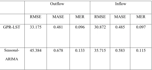
Table 1: Outflow vs Inflow ( NYC’s Workdays) ... 70

Table 2: Workdays vs Weekends (NYC’s outflow)... 71

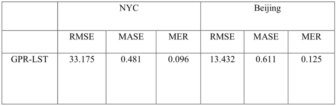
Table 3: NYC vs Beijing (Outflow in the workdays) ... 72

LIST OF FIGURES

Figure 1.1 an overview of the proposed methodology ... 9

Figure 2.1 Snapshots of San Francisco traffic ... 15

Figure 2.2. Illustrations of trajectory data ... 19

Figure 2.3 Execution overview of MapReduce model (Dean and Ghemawat 2008) ... 26

Figure 3.1. Higher-order orthogonal iteration algorithm... 32

Figure 3.2 Tensor model of human spatial-temporal movements ... 33

Figure 3.3 Tensor factorization ... 34

Figure 4.1: An illustration of a trajectory distribution ... 42

Figure 4.2 Some possible trajectories for a given origin-destination pair. ... 47

Figure 6.1: Pick-up and drop-off activities of NYC in a single day ... 66

Figure 6.2: Taxi activities of Beijing in a single day ... 68

Figure 6.3. Prediction error at different time periods ... 75

Figure 6.4 The prediction error (MASE) at different spatial units ... 78

Figure 6.5 The number of pick-ups and drop-offs vs. prediction error (MASE) ... 79

Figure 6.7 The clustered neighborhoods of NYC ... 83

Figure 6.8 The clustered neighborhoods of Beijing ... 83

Figure 6.9 Average hourly inflow/outflow of selected neighborhoods... 85

Figure 6.10 Prediction error(MER) at different time periods ... 87

Figure 6.11: Prediction error (MASE) at different time periods... 87

Figure 6.12 Prediction error with different Training Data Lengths ... 88

Figure 6.13 Prediction of hot road segments. ... 92

Figure 6.14 Prediction of Top-K origin/destination neighborhoods. ... 93

Figure 6.15 Running time of trajectory distribution simulation vs number of reducers. .. 96

Figure 6.16 Running time of trajectory distribution analysis versus the number of reducers. ... 96

1.0 INTRODUCTION

A large amount of spatial-temporal data related to human mobility accumulates daily from all kinds of city infrastructures, because of the rapid development and common use of location-sensing technologies, such as GPS and RFID sensors. Solving many real-world problems requires understanding and correctly predicting these spatial-temporal activities (for example, the outflow/inflow of people), as well as these movements’ trajectory distributions in the road network. For example, by predicting the number of people who would leave or enter certain neighborhoods during the next half hour, taxi companies or Uber can optimally allocate their vehicles. Correspondingly, traffic agencies could further investigate and simulate these vehicle movements’ corresponding trajectories in the road network and find the set of hot road segments with high centrality where lots of vehicles would pass by, from which future traffic congestions and their possible causes, among other things, can be predicted even before it happens. For example, based on the prediction, a high percentage of vehicles that travel from region A/B heading to region C/D might pass the same route in the next half hour, which would indicate a possible traffic jam or bottleneck there later—and as a result, we could send suggestions to some of those drivers to avoid this route if possible.

These problems pose many technical challenges. First, in order to predict spatial-temporal activities (for example, people’s outflow/inflow in the urban environment), one natural approach is to identify both the spatial and temporal features of these activities and use these features to train a predictive model for future prediction. However, the mix of spatial and temporal patterns among human activities makes it difficult to identify and extract the spatial and temporal features, respectively, from existing mobility datasets. By assuming overall spatial and temporal closeness, many existing techniques use the information from adjacent spatial areas and recent time periods as the spatial and temporal features for prediction (Williams and Hoel 2003, Froehlich, Neumann et al. 2009, Kaltenbrunner, Meza et al. 2010, Chen, Hu et al. 2011, Nishi, Tsubouchi et al. 2014). However, there are a few problems with such methodologies. For example, there is no definition of how close two areas should be to one another in order to share a similar pattern, and also, close areas do not necessarily share a similar pattern. Existing works have similar problems with temporal characteristics. At the same time, it is difficult for these exiting methods to inherently take both spatial and temporal characteristics into consideration, given that spatial and temporal features have different scales and that there are unknown relationships between them and human mobility.

As for the second problem (the simulation of corresponding movements’ trajectory distribution in the road network and the detection of hot road segments with high centrality), it poses many technical challenges in the areas of uncertainty and big data. First, we would need to accurately predict the flow of people across neighborhoods.

To infer their corresponding trajectory distributions in the road network, we would need to know how many people leave a place and their probable trajectories. However, considering that there are usually multiple routes from which people can choose from one place to another, it is hard to tell which route people might follow and/or the corresponding possibilities of them following each particular route. Besides this overall uncertainty, the scale of a city’s road network and the number of trajectories that people usually take during certain time periods could be quite large. Take New York City as an example. There are 388,409 road intersections and 523,442 road segments (OpenStreetMap 2017). In 2001, people made approximate 209 million vehicles trips (a trip by a single privately operated vehicle) and traveled 3 billion vehicle miles (one vehicle mile of travel is the movement of one privately operated vehicle for one mile, regardless of the number of people in the vehicle) (Patricia S. Hu 2001). As for taxi cabs (one of the most important transportation modes in New York City), each day they carry over one million passengers and make, on average, 500,000 trips—adding up to 170 million trips during 2011 (Ferreira, Poco et al. 2013). These numbers indicate that the task of predicting a city level’s trajectory distribution is computationally intensive and would require efficient algorithms for real-time responses.

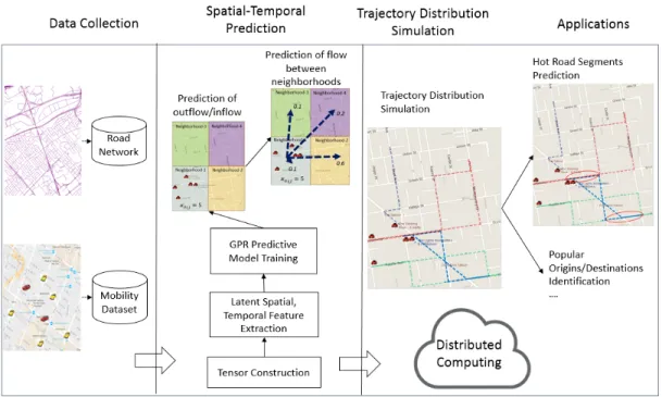
To tackle these challenges, this dissertation proposes a comprehensive methodology for the prediction of large scale of human spatial-temporal mobility, especially a city level’s trajectory distributions in the road network. An overview of our

methodology is given in Figure 1.1. Specifically, our methodology comprises several specific components.

First, we propose a novel methodology for prediction of spatial-temporal activities (such as human outflow/inflow and their corresponding destination/origin distribution) using the latent spatial and temporal features extracted through tensor factorization, given historical mobility datasets. One major motivation behind our methodology is that we suspect the patterns of many spatial-temporal activities, such as human mobility, are highly correlated to or dependent on the characteristics of spatial environments, temporal periods, and other factors. For example, residential neighborhoods and office districts have high volumes of outflow and inflow in the morning and in the evening, respectively. While this is an interesting observation analyzed qualitatively, it is not sufficient to allow for any prediction, such as the number of people who would be leaving/entering a residential neighborhood during certain time periods. With our proposed methodology, we can use this simple initial qualitative information to predict various spatial-temporal activities. In particular, we first identify and quantify the latent characteristics of different spatial environments and temporal factors through tensor factorization. Next, we propose to model the hidden relationship between spatial-temporal activity and extract latent features as a Gaussian process, which can be viewed as a distribution over the possible functions. One major advantage of this proposed methodology is that it inherently considers both spatial and temporal data characteristics. In particular, through mathematically modeling the characteristics of

different spatial areas, different time periods, and their relationship to mobility patterns as a Gaussian process, predictions can be made using the data from not only one specific spatial area or temporal time period of interest, but also from other areas and time periods with similar patterns.

After predicting the flow of people between neighborhoods, we further investigated and simulated those movements’ corresponding trajectories in the road network, from which we could predict some important phenomenon, for example, finding a set of road segments that many vehicles would use and identify the causes or reasons for their heavy use, such as the origins or destinations of the majority of the traffic in those road segments. Given that there are usually multiple routes that people can choose to go from one place to another, there is a challenge of uncertainty. Some previous works (Matthias and Zuefle 2008, Ren, Ercsey-Ravasz et al. 2014, Deri and Moura 2015) assumed people always choose the shortest paths. However, this might not be the case since people seldom strictly follow the shortest paths in their daily driving. To bridge the gap, we propose several models of vehicles’ trajectory distributions in the road network, such as one based on the multivariate kernel density estimation. We provided a case study of Beijing’s taxi data and compared our proposed models with traditional models, such as the shortest path. Experimental results demonstrate the advantage of our proposed model.

It is worth pointing out that the problems discussed above are very computationally intensive when considering the scale of a city’s road network and the

numerous trajectories that people might take during a certain time period. With the advent of emerging cloud technologies, a natural and cost-effective approach to manage such large-scale data is to store them in a cloud environment and process them using modern distributed computing paradigms, such as MapReduce (Dean and Ghemawat 2008). In this work, different MapReduce-based distributed algorithms are proposed for (1) simulating vehicle trajectory distributions in the road network, based on the predicted outflow/inflow movements between neighborhoods from the previous step; and (2) analyzing the synthetic large-scale trajectory distributions in order to find interesting phenomena, such as the road segments that many vehicles might use, as well as the causes of these phenomena, like the origin and destinations of the majority of the traffic.

It should be pointed out that a trajectory is a unique way to represent people’s spatial-temporal activity. It can be viewed as a sequence of time-ordered location records, such as a series of GPS points with latitude and longitude, or as a sequence of connected road segments in the road network. There are many techniques developed to predict a single vehicle’s future trajectory, based on its initial partial trajectory (Liu and Karimi 2006, Froehlich and Krumm 2008, Chen, Lv et al. 2010, Jeung, Yiu et al. 2010). One major difference between these existing works and the proposed work in this thesis is that we focus more on people’s/vehicle’s movements at a city level and the corresponding trajectory distributions, instead of on a single vehicle’s personal routing preference in the road network, based on its partial initial trajectory and history patterns. For several reasons, these personal predictions cannot be aggregated to achieve a city-level prediction.

First, the mobility problem addressed in this paper is quite different from those that have been addressed in previous works. In particular, most existing works seek to answer the question: Given a partial initial trajectory of a vehicle already in the road network, what is its most likely future trajectory in the road network? However, our methodology tries to answer the questions: How many people are heading from one specific neighborhood to another in the near future, say in the next hour?; What are the probable trajectories of these movements?; Which road segments would have a high degree of centrality (a lot of vehicles would pass by) and result in traffic jams?; and What are the origins and destinations of the traffic that passes through those hot road segments? Besides, due to privacy and technical issues, it is difficult to collect and store everyone’s trajectory at the necessary level of detail (such as every two minutes) at the city level. On the other hand, some mobility datasets with less detail (namely, those with only origin and destination information for each trip) are more widely available, such as the census data/travel survey (Jiang, Ferreira Jr et al. 2012), mobile phone records (Gao, Liu et al. 2013), check-ins from location-based social networks such as Foursquare (Wei, Zheng et al. 2012), and others. Our proposed methodology is flexible and can properly handle both cases. Finally, the scale of the problem (a city-level trajectory distribution computation) is computationally intensive and requires efficient distributed algorithms to achieve suitable performance.

There are also some other related works, such as those that include the discovery of popular trajectories or hot routes from historical datasets (Li, Han et al. 2007, Chen,

Shen et al. 2011, Wei, Zheng et al. 2012, Han, Liu et al. 2015) and an estimation of the current traffic situation from Twitter (Sayyadi, Hurst et al. 2009, Castro, Zhang et al. 2012, Chen, Chen et al. 2014, Liu, Fu et al. 2014, Wang, Li et al. 2016). While these proposed techniques can find some interesting phenomena, such as popular routes and traffic jams that have previously happened or that are happening at the moment, they provide little assistance to future predictions. For example, there could be a local event in a neighborhood today with several road segments blocked by the police, which would cause some of the nearby roads to be congested with a higher traffic volume than usual— or maybe not, depending on people’s mobility at that time and the nearby road network topology. Mining historical hot routes cannot predict these abnormal situations. On the other hand, with the proposed methodology in this work, we can predict people’s flow volume across neighborhoods at a city level, simulate their corresponding trajectories in the road network by blocking corresponding road segments, and check to see if any nearby road segments would become crowded or remain clear.

The proposed methodology in this paper could also shed light on a future Intelligent Transportation System prototype that would help alleviate traffic congestion problems in metropolitan cities. Specifically, as self-driving vehicles become feasible and even prevalent in the future, our methodology could be used in a public cloud environment, where self-driving vehicles on the road network would act as the clients and send their movement information to the cloud in advance, including both their origins and destinations. The cloud would aggregate this information, estimate the trajectory

distribution in the road network based on the routing strategies of self-driving vehicles, and detect the corresponding levels of traffic. If a congestion is predicted (too many vehicles would try to use the same route in the near future), the cloud would send this information to affected self-driving vehicles so that they could update their routes (choose less crowded routes).

1.1 Research Problems

This thesis tackles the challenges of the prediction of human mobility on a large scale. In particular, we focus on people’s spatial-temporal mobility of outflow/inflow, and their trajectory distributions in the road network, from which we could optimally reallocate transportation resources, such as taxis or Uber vehicles, and estimate future traffic situations, such as congestion and its possible causes, among others. In particular, this research addresses the following questions:

1. How can we quantify the features of the spatial and temporal factors, based on the existing mobility dataset?

2. How can we mathematically model the relationship between the extracted spatial-temporal features and people’s mobility, such as outflow/inflow in an urban environment, for future predictions?

3. How can we accurately model people’s trajectory distributions in the road network based on the previous predicted flows?

4. How can we efficiently simulate the huge amount of movement trajectory distributions in a city level’s road network?

5. How can we efficiently process the large scale of trajectory distributions generated from previous steps for some useful information, such as predicting the

set of hot road segments and identifying where the majority of traffic in those road segments are coming from or going to?

1.2 Contributions

The research in this thesis has six major contributions:

(1) A comprehensive methodology for the prediction of people’s mobility at a large scale.

(2) A novel model to predict temporal activity using latent spatial-temporal features extracted from existing mobility data.

(3) Different models for the estimation of vehicle trajectory distributions in a road network.

(4) A distributed algorithm for the real-time simulation of large-scale trajectory distributions in a road network.

(5) Different distributed algorithms for the processing and analysis of large-scale trajectory distribution, such as the prediction of hot road segments that are based on such analyses.

(6) Case studies based on real-world data collected from New York City and Beijing’s taxi trip data sets.

1.3 Chapters Overview

The rest of the proposal is organized as follows. Section 2 reviews background information and related work. Section 3 presents the proposed novel methodology for the prediction of human spatial-temporal mobility, using latent features. Section 4 presents the models of trajectory distributions in the road network. Section 5 provides different MapReduce-based distributed algorithms, including the simulation of the corresponding trajectory distributions in the road network and the analysis of the simulated trajectory distributions, such as the prediction of hot road segments. Section 6 conducts case studies with data sets of taxi trips taken in both New York City and Beijing, and systematically evaluates our proposed methodology. Section 7 provides the conclusions of this thesis and future research direction.

2.0 BACKGROUND AND RELATED WORK

Issues of human mobility have attracted lots of attention for a long time from researchers in a wide variety of fields, such as urban planning, sociology, computer science, and geology, among others. This chapter reviews how existing work analyzes and predicts human spatial-temporal activities from different perspectives, their limitations, and the difference between them and the proposed work in this thesis.

2.1 Traffic Prediction

Traditionally, researchers have used static models, such as the gravity model (Wilson 1967), to estimate the amount of interactions between two geographic areas, such as two cities. With the invention of some infrastructure sensors, such as a traffic loop that can count the number of vehicles passing a road segment, these models have been widely deployed in cities’ road networks. Many models have been developed to predict the traffic situation from these data. Davis and Nihan (Davis and Nihan 1991) suggested a nonparametric k-nearest neighborhood approach to predict short-term traffic volume. The general idea is to use the recent traffic volume from a to-be predicted freeway and its

adjacent freeways as the input vector, to find the top-k closest vectors in history, and compute the average value. Clark (Clark 2003) proposed a similar k-NN approach, but with more input variables and different outputs; besides the traffic volume, this model also collects and predict the speed, flow, occupancy, and other factors, as well as explores the accuracy between different univariate or multivariate models. Williams and Hoel (Williams and Hoel 2003) presented the theoretical basis for modeling univariate traffic condition data streams as seasonal autoregressive integrated moving average processes. Shekhar and Williams (Shekhar and Williams 2008) presented an adaptive parameter estimation methodology for univariate traffic condition forecasting through the use of three well-known filtering techniques: the Kalman filter, recursive least squares, and least mean squares.

One limitation of these works is that they can only predict the traffic volume of a single road segment in isolation, and cannot provide any other information, such as the causes of possible traffic jams or the patterns of people’s mobility at a higher level, leaving the question open as to where the traffic in those road segments is coming from or where it is going. This information would help traffic agencies optimize the traffic resource more efficiently. Figure 2.1 (Li, Han et al. 2007) gives a good example of this issue. It shows traffic data in the San Francisco Bay Area on a weekday at approximately 7:30 am local time. Different colors show different levels of congestion (for example, dark red shows heavy congestion). We can see that there are some congestions in the road network, but we do not know why this congestion is occurring. If we can predict that

traffic jams are formed because many people are driving from location Y to location X, the traffic agencies could increase the frequency of corresponding public buses traveling from Y to X during those time periods to reduce the volume of private traffic.

(a) The Bay Area (b) A closer look at the congested area Figure 2.1 Snapshots of San Francisco traffic

Besides these limitations, the high cost of deploying and maintaining the infrastructure of traffic loops also limits their coverage. Motivated by the popularity of location-based applications and social networks such as Twitter, many recent studies have been conducted to explore these social media data for its use in estimating traffic situations. The core idea of this field is to detect traffic-related tweets and use them to

estimate the current traffic situation. Sayyadi et al. (Sayyadi, Hurst et al. 2009) proposed and developed an event-detection algorithm which creates a keyword graph and uses community detection methods analogous to those used for social network analysis to discover and describe events. Liu et al. (Liu, Fu et al. 2014) presented an application for traffic event detection and summaries, based on mining representative terms from the tweets posted when anomalies occur. Chen et al. (Chen, Chen et al. 2014) presented a unified statistical framework that combines two models based on hinge-loss Markov random fields (HLMRFs) to monitor traffic congestion through feeds from tweet streams. Although using crowd-sourced data from social networks have some advantages in some cases, these existing methodologies also have limitations such as failing to detect many ongoing traffic events, due to the sparsity of traffic-related information on social networks (since few people are likely to tweet about the traffic situation while driving) and they also gain little insight of people’s travelling patterns. In addition to these limitations, the proposed technique in this thesis and the works above also have different foci. Those works previously cited focus more on the estimation of the current traffic situation through extracting the traffic-related information from the tweets that people posted about their current traffic situations. However, our proposed methodology focuses more on the prediction of future movements; people’s outflow/inflow across neighborhoods, their corresponding possible trajectory distribution in the road network, and the set of hot road segments where lots of vehicles might pass by in the near future.

There are also some other related works such as the abnormal spatial events detection, e.g., people’s gathering events. (Neill 2009) proposed a two-step approach based on the expectation-based scan statistic for the detection of emerging spatial patterns through monitoring a large number of spatially localized time series. (Hong, Zheng et al. 2015) modeled human mobility as Spatio-Temporal Graph (STG) for the detection of phenomena, entitled black holes and volcanos. Specifically, a black hole is a subgraph (of STG) that has the overall inflow greater than the outflow by a threshold while volcanos is the other way around. (Zhou, Khezerlou et al. 2016) proposed a model of Gathering directed acyclic Graph (G-Graph) for the early detection of gathering events. To improve the computation efficiency, they also designed an algorithm called SmartEdge.

Apart from vehicles’ traffic in the road network, there are also some studies on other modes of transportation or urban activity such as pedestrians, shared bicycle system, etc. Nishi et al. (Nishi, Tsubouchi et al. 2014) described a statistic-based method to estimate trends in the pedestrian population using location data collected from Yahoo! Japan app users. Froehlich et al. (Froehlich, Neumann et al. 2009) provided a spatial-temporal analysis of bicycle station usage in Barcelona and compared experimental results from four simple predictive models. Kaltenbrunner et al. (Kaltenbrunner, Meza et al. 2010) also provided spatial-temporal analysis for bicycle usage in Barcelona and adopted an autoregressive-moving-average (ARMA) model to predict the number of bikes and docks available at each bike station.

2.2 Trajectory Mining

The pervasive use of location-sensing technology such as GPS receivers and WiFi embedded in mobile devices has led to the accumulation of huge amounts of trajectory data. Generally, a trajectory can be viewed as a sequence of data points with location information (Figure 2.2a) or as road segments (Figure 2.2b).

(b) Trajectory of road segments Figure 2.2. Illustrations of trajectory data

2.2.1 Individual Trajectory Predictions

Among the various topics in the field of trajectory mining, predicting the future trajectory of a person or vehicle is of great interest. Liu and Karimi (Liu and Karimi 2006) presented two models for trajectory prediction: a probability-based model and a learning-based model. Froehlich and Krumm (Froehlich and Krumm 2008) developed the algorithms for predicting the end-to-end route of a vehicle, mainly based on GPS observations of the vehicle’s past trips. Jeung et al. (Jeung, Yiu et al. 2010) presented a maximum likelihood and a greedy algorithm for predicting the travel path of an object, based on a developed mobility model that offers a concise representation of mobility

statistics extracted from massive collections of historical object trajectories. Scellato et al. (Scellato, Musolesi et al. 2011) created a spatial-temporal location prediction model for a single user, based on his/her own historical trajectories. Zhang et al. (Zhang, Lin et al. 2016) introduced EigenTransitions, a spectrum-based, generic framework for analyzing mobility datasets and predicting an individual user’s mobility, such as the next area they are likely to visit. As discussed above, the major application of these studies was to predict a single vehicle’s personal routing preference in the road network, based on its partial initial trajectory and history patterns. On the other hand, the proposed work in this thesis focuses on people’s movements at a city level and their corresponding trajectory distributions, which is computationally intensive. As a result, an efficiently distributed solution is needed. Furthermore, due to privacy and technical issues, it is difficult to frequently collect a series of GPS points from many individual users to gain an overview of a city level’s mobility and the corresponding traffic situation in the near future, as with the input data required by these studies; in contrast, our methodology can handle some less detailed datasets, such as a huge number of anonymous trips with only origins, destinations, and their corresponding timestamps.

2.2.2 Popular Trajectory Mining

Mining popular routes from existing trajectory datasets is another topic that is close to our proposed methodology. Li et al. (Li, Han et al. 2007) proposed a density-based algorithm named FlowScan to cluster road segments based on the density of common

traffic they share. Zhu et al. (Zhu, Luo et al. 2010) proposed a novel three-phase approach to discover a tropical cyclone’s trajectory corridors, based on clustering methods. Chen et al. (Chen, Shen et al. 2011) investigated the most popular route (MPR) between two locations by observing the traveling behaviors of many previous users. They developed an algorithm to retrieve a transfer network from raw trajectories that would indicate all the possible movements between locations. After that, the absorbing Markov chain model is applied to derivea reasonable transfer probabilityfor each transfer node in the network. Comito et al. (Comito, Falcone et al. 2015) defined and implemented a novel methodology to mine popular travel routes from geo-tagged posts. Han et al. (Han, Liu et al. 2015) designed a road-network aware approach, named NEAT, for the fast and effective clustering of trajectories of mobile objects travelling in road networks. More specifically, NEAT can discover spatial clusters as groups of sub-trajectories that describe both dense and highly continuous flows of mobile objects.

Compared with our proposed methodology in this thesis, these existing techniques focus on mining phenomena such as popular routes or historical traffic jams, but cannot provide much information for future situations, especially when some of conditions change. For example, there might be a parade in a neighborhood this afternoon that would cause several road segments to be blocked by the police, which could lead to a drastic change in trajectory patterns. In order to estimate the overall impact of such an event, the city agencies can use our proposed methodology to predict people’s movements and simulate the corresponding trajectory distributions by blocking those

road segments, so they could check if any of nearby road segments would become too crowded.

2.2.3 Other Trajectory Mining

Other studies have also been conducted to mine trajectory datasets to reveal different interesting urban activities. Guo et al. (Guo, Liu et al. 2010) developed a graph-based approach that converts trajectory data to a graph-based representation and treats it as a complex network, to which they further apply a spatially constrained graph partitioning method to discover natural regions defined by trajectories. Liu et al. (Liu, Liu et al. 2010) presented a novel, non-density-based approach called mobility-based clustering to identify hot spots of moving vehicles in an urban area. The key idea is to use the sample objects’ instant mobility (taxi trajectory data) as the “sensors” to perceive the vehicle density in nearby areas. Liu et al. (Liu, Zhu et al. 2012) proposed a novel algorithm for recognizing urban roads with coarse-grained GPS traces from probe vehicles moving in urban areas. Zhang et al. (Zhang, Wilkie et al. 2013) proposed a step toward real-time sensing of refueling behavior and citywide fuel consumption using the reported trajectories from a fleet of GPS-equipped taxicabs. Wang et al. (Wang, Zheng et al. 2014) presented a citywide and real-time model for estimating the travel time of any path in real time in a city, based on the GPS trajectories of vehicles received in current time slots and over a period of history, as well as information from map data sources.

2.3 Urban Community and Event Analysis

In addition to the trajectory dataset, exploring and discovering hidden interesting phenomena based on other spatial-temporal datasets, such as location-based social networks, has also attracted much attention. Spatial community discovery/analysis is one of the hottest research topics, among others. Cranshaw et al. (Cranshaw, Schwartz et al. 2012) introduced a clustering model and research methodology for studying the structure and composition of a city on a large scale, based on the social media information that its residents generate. Noulas et al. (Noulas, Scellato et al. 2011) also proposed an approach to cluster geographic areas with similar categories. This study also clustered the users according to the types of places they check in and the frequency of check-ins. Yuan et al. (Yuan, Zheng et al. 2012) proposed a framework (titled DRoF) that discovers regions of different functions in a city, using both human mobility among regions and points of interests (POIs) located in a region.

Many other interesting phenomena have been explored besides the spatial community. Comito et al. (Comito, Falcone et al. 2015) proposed a methodology to infer interesting locations and frequent travel sequences among these locations in a given geo-spatial region from geo-tagged tweets. Kamath et al. (Kamath, Caverlee et al. 2012) explored how the factors of spatial influence and interest affinity affect the global spread of social media. Noulas and Mascolo (Noulas and Mascolo 2013) inferred the functions

of each neighborhood in the city by using Foursquare POIs and cellular data. Finally, Quercia et al. (Quercia, Aiello et al. 2015) explored the possibilities of using social media data from Flickr and Foursquare to automatically identify safe and walkable streets.

Other datasets, such as phone usage, census-based data, and public transportation records, among others, have also attracted much attention, in addition to location-based social networks. Lathia et al. (Lathia, Quercia et al. 2012) explored the correlation between London’s urban flow of public transport and the well-being of London’s census areas (measured by census-based indices), from which some phenomena are found, such as a segregation effect. Lam and Bouillet (Lam and Bouillet 2014) proposed an efficient real-time algorithm to cluster the events generated by the sensors available from traffic light control systems, which are composed of an induction loop which is triggered whenever a metallic object is detected, such as a car. Zheng et al. (Zheng, Liu et al. 2014) inferred the fine-grained noise situation at different times of day for each region of NYC by modeling the noise situation of NYC with a three-dimensional tensor and supplementing the missing entries of the tensor through a context-aware tensor decomposition approach. Finally, Liu et al. (Liu, Wang et al. 2012) derived urban land-use information by classifying the study area into six types of “source-sink” areas through taxi data on pick-ups and drop-offs in Shanghai.

2.4 Distributed Computing

Since the scale of many spatial-temporal datasets nowadays could be as large as tens of hundreds of gigabytes (or even larger), creating a real-time query and prediction method to use this large amount of data poses great challenges for a single commodity computer. As cloud computing has emerged as a cost-effective and promising solution for both computing- and data- intensive problems, a natural approach to manage such large-scale data is to store and process these datasets in a cloud service using modern distributed computing paradigms such as MapReduce.

2.4.1 MapReduce

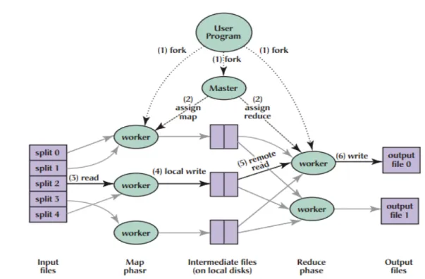
MapReduce is a programming model and an associated implementation for processing and generating large datasets that is amenable to a broad variety of real-world tasks (Dean and Ghemawat 2008). Hadoop is a popular open source implementation of the MapReduce framework. Hadoop is composed of two major parts: the storage model (the Hadoop distributed file system , or HDFS), and the compute model (MapReduce). Figure 2.3 shows an execution overview of the MapReduce model.

Figure 2.3 Execution overview of MapReduce model (Dean and Ghemawat 2008)

A key feature of the MapReduce framework is that it can distribute a large job into several independent maps, and reduce tasks over several nodes of a large data center and process them in parallel. At the same time, MapReduce can effectively leverage data locality and processing on or near the storage nodes, and results in faster execution of the jobs. The framework consists of one master node and a set of worker nodes. In the map phase, the master node schedules and distributes the individual map tasks to the worker nodes. A map task executed in a worker node processes the smaller chunk of the file stored in HDFS and passes the intermediate results to the appropriate reduce tasks that are being executed in a set of worker nodes. The reduce

tasks collect the intermediate results from the map tasks and combine/reduce them to form the final output. Since each map operation is independent of the others, all map tasks can be performed in parallel. The same process occurs with reducers, as each reducer works on a mutually exclusive set of intermediate results produced by mappers.

2.4.2 Spatial Data Processing in Hadoop

Since MapReduce/Hadoop has become the defacto standard for distributed computation on a massive scale, some recent works have developed several MapReduce-based algorithms for spatial problems. Puri et al. (Puri, Agarwal et al. 2013) proposed and implemented a MapReduce algorithm for distributed polygon overlay computation in Hadoop. Ji et al. (Ji, Dong et al. 2012) presented a MapReduce-based approach that constructs an inverted grid index and processes kNN query over large spatial data sets. Akdogan et al. (Akdogan, Demiryurek et al. 2010) designed a unique spatial index and Voronoi diagram for given points in 2D space, which enables the efficient processing of a wide range of geospatial queries, such as RNN, MaxRNN and kNN with the MapReduce programming model. (Guo, Palanisamy et al. 2014) developed a MapReduce-based parallel polygon retrieval algorithm which aims to minimize the IO and CPU loads of the map and reduce tasks during spatial data processing. Hadoop-GIS (Wang, Lee et al. 2011) and Spatial-Hadoop (Eldawy, Li et al. 2013, Eldawy and Mokbel 2013) are two scalable, high-performance spatial data processing systems for running large-scale spatial queries

in Hadoop. These systems provide support for some fundamental spatial queries, such as the minimal bounding box query.

However, these studies only support some static spatial queries. They do not support spatial-temporal trajectory predictions, simulations, and the corresponding discovery of hot road segments that are addressed in this thesis. As a result, we propose to devise specific optimization techniques for an efficient implementation of the parallel trajectory prediction and simulation functions in MapReduce.

3.0 NOVEL SPATIAL-TEMPORAL PREDICTION USING LATENT FEATURES

In this section, the spatial-temporal prediction methodology that uses the latent features will be presented in detail. First, we describe how to model people’s spatial-temporal fluxes as a tensor and extract the latent spatial-temporal features through factorization. Then, we present how to mathematically model the relationship between those extracted latent features and human mobility using a Gaussian process regression for future prediction.

3.1 Tensor Model of the Spatial-Temporal Activities

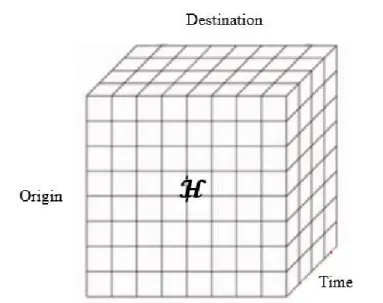
A tensor is a multidimensional array. Decompositions of a higher-order tensor can be used to extract and explain the properties among the tensor, which have wide applications in computer vision, numerical analysis, data mining, neuroscience, graph analysis, and elsewhere (Kolda and Bader 2009). In this thesis, we propose to model human fluxes between different neighborhoods with a 3-dimensional tensor ℋ ∈ ℛ𝑁×𝑁×𝐿_{, as shown in} Figure 3.2. The first dimension of the tensor ℋ denotes 𝑁 origin neighborhoods, the

second dimension denotes 𝑁 destination neighborhoods, and the third dimension denotes 𝐿 time slots, respectively. Each entry of the tensor ℋ(𝑖, 𝑗, 𝑙) stores the average number of trips starting from neighborhood 𝑖 to neighborhood 𝑗 during time period 𝑙.

With this tensor model, we extract the latent spatial features of each origin neighborhood, destination neighborhood, and the latent temporal feature of each time slot through a Tucker decomposition. The Tucker decomposition can be thought of as the form of higher-order Principal Component Analysis (PCA). It decomposes a tensor into a core tensor multiplied by a matrix along each dimension (Kolda and Bader 2009). In our case, we decompose the tensor ℋ into three matrices 𝒮𝑜𝑁×𝑃, 𝒮𝑑𝑁×𝑄, 𝒯

𝐿×𝑅

, and a core tensor 𝐺𝑃×𝑄×𝑅_{, respectively, as shown in Figure 4.3. Mathematically, this relationship} can be expressed as in Equation 3.1:

ℋ ≈ 𝐺 ×₁𝒮_𝑜×₂𝒮_𝑑×₃𝒯 = ∑ ∑ ∑ 𝑔_{𝑝 𝑞 𝑟 𝑝𝑞𝑟}𝒮_𝑜:,𝑝°𝒮_𝑑:,𝑞°𝒯_:,𝑟 (3.1)

Each element ℋ is:

ℎ_𝑖𝑗𝑙 ≈ ∑ ∑ ∑ 𝑔_{𝑝 𝑞 𝑟 𝑝𝑞𝑟}𝒮_{𝑜𝑖,𝑝}𝒮_{𝑑𝑗,𝑞}𝒯_𝑙,𝑟 (3.2)

Here, the symbol "°" stands for the vector outer product, which means that each element of the tensor is the product of the corresponding vector elements. 𝒮_𝑜:,𝑝 indicates the 𝑝𝑡ℎ _{column of matrix 𝒮}

𝑜 and 𝒮𝑜𝑖,𝑝 is the 𝑖𝑡ℎ element in the 𝑝𝑡ℎ column. 𝒮𝑜, 𝒮𝑑 and 𝒯 are the factor matrices and can be viewed as the principal component of the tensor’s three corresponding dimensions. In other words, the row 𝑖 of matrix 𝒮𝑜, 𝒮𝑜𝑖,:, is the feature vector that indicates the characteristics of origin neighborhood 𝑖. Similarly, the row 𝑗 of

matrix 𝒮𝑑, 𝒮𝑑𝑗,:, is the feature vector that indicates the characteristics of destination neighborhood 𝑗. 𝒯_𝑙,:, is the feature vector that indicates the characteristics of the corresponding time slot 𝑙. Each entry of the core tensor 𝐺 indicates the level of interaction among different components of 𝒮_𝑜, 𝒮_𝑑, and 𝒯, respectively.

This decomposition problem can be turned into an optimization problem: min ||ℋ -𝐺 ×1𝒮𝑜×2𝒮𝑑×3𝒯||2 (3.3)

subject to 𝐺 ∈ ℛ𝑃×𝑄×𝑅_, 𝒮_𝑜 ∈ ℛ𝑁×𝑃_,

𝒮_𝑑 ∈ ℛ𝑁×𝑄,

𝒯 ∈ ℛ𝐿×𝑅

To solve this optimization problem, (De Lathauwer, De Moor et al. 2000) designed a higher-order orthogonal iteration algorithm. In our case, the algorithm is shown in Figure 3.1:

Figure 3.1. Higher-order orthogonal iteration algorithm

The motivation behind using the tensor factorization is that we think the existence of some latent features and interactions among them usually determine the patterns of many spatial-temporal activities such as how people in one neighborhood (origin) move to another neighborhood (destination) during certain time periods. For example, two residential neighborhoods would both have a high volume of outflow (to an office district) in the morning. Similarly, two nightlife districts would both attract a high volume of inflow in the evening. This is a simple qualitative analysis that is difficult to extend to general cases, since most regions are not monofunctional and people’s flow is usually a mix of a variety of life patterns. However, by discovering the latent features and the interactions among them, we can mathematically model people’s movements with respect to a certain neighborhood during certain time periods for future prediction. This is

somewhat similar to the recommendation system like the one Netflix uses, where a multidimensional tensor represents how different users rate different movies under various contexts, such as different times. For example, two users might give a high rating to a certain movie if they both liked the actors/actresses in the movie, or if the movie was a romantic movie, which was preferred by both users in the previous couple of weeks. Hence, if we can discover these latent features, we should be able to predict a rating with respect to a certain user and a certain item under specific contexts. Similarly, given the extracted latent features of origin neighborhoods (like users), destination neighborhoods (like movies), the specific time period, and some other features, we could predict people’s flow.

Figure 3.3 Tensor factorization

3.2 Prediction Using Gaussian Process Regression (GPR)

3.2.1 GPR Model between Spatial-Temporal Activities and Latent Features

After the extraction of latent spatial-temporal features, we mathematically model the relationship between spatial-temporal activities such as human mobility and the extracted latent features for prediction. For this, we assume that people’s mobility is generated from a smooth and continuous process. This process has typical amplitude and variations in the function which takes place over spatial, temporal, and other characteristics. For

example, to predict the volume of outflow 𝓍_{𝑜𝑖,𝑙} in the neighborhood 𝑖 during time period

𝑙 (or the volume of inflow 𝓍_{𝜄𝑖,𝑙}), we can model the relationship as below:

𝓍_{𝑜𝑖,𝑙}= 𝑔(𝒮_𝑜𝑖,:, 𝒯_𝑙.:, 𝓍_{𝑜𝑖,𝑙−1}, … ) (3.4) 𝓍_{𝜄𝑖,𝑙} = 𝑔(𝒮_𝑑𝑖,:, 𝒯_𝑙,:, 𝓍_{𝜄𝑖,𝑙−1}, … ) (3.5)

Note that instead of relating this relationship to some specific models such as linear, quadratic, cubic, or even non-polynomial models, which may have numerous possibilities, we modeled this relationship as a free-form Gaussian process. One reason for using the Gaussian process is that for any spatial-temporal activity 𝑦 (e.g., 𝓍_{𝑜𝑖,𝑙}) to be predicted, it will likely be generated by the same process and have similar values as the historical processes that share similar latent spatial-temporal features. We can take advantage of this relationship and use it for prediction. Formally, the Gaussian process can be represented as (Rasmussen 2006):

𝑦⃗~𝑔(𝕏 )~𝐺𝑃 (𝑚(𝕏), 𝐾(𝕏 , 𝕏)) (3.6)

where 𝑦⃗ is a vector that contains a series of spatial-temporal activities

(𝑦₁, 𝑦₂, … , 𝑦_𝑛), 𝕏 is the features matrix of 𝑦⃗ (here for an activity 𝓍_{𝑜𝑖,𝑙}, the corresponding

feature in 𝕏 would be (𝒮_𝑜𝑖, 𝒯𝑙, 𝓍𝑜𝑖,𝑙−1,…)); 𝑚(𝕏) is the expected value of the generating process 𝑔(𝕏); and 𝐾(𝕏, 𝕏) is the covariance matrix where its element 𝑘_𝑖,𝑗 measures the similarity between the input features of activity 𝑦_𝑖 and 𝑦_𝑗. We can also represent the relationship above as:

𝑝(𝒚(𝕏)) ~ 𝒩(𝑚(𝕏), 𝐾(𝕏 , 𝕏)) (3.7) For a future activity 𝑦∗ _{to be predicted, we have:}

𝑝 (_𝑦𝑦⃗⃗∗)~ 𝒩((_𝑚(𝕏𝑚(𝕏)∗₎) , [ 𝐾 𝐾 ∗𝑇

𝐾∗ _𝐾∗∗]) (3.8)

where 𝐾, 𝐾∗_{, and 𝐾}∗∗ _{are the abbreviations of the covariance matrix 𝐾(𝕏, 𝕏),}

𝐾(𝕏∗, 𝕏), and 𝐾(𝕏∗_{, 𝕏}∗_{), respectively, and 𝑇 indicates a matrix transposition. The key}

ideas in Equation-3.7 and Equation-3.8 are that we assume that future data are generated from the same process as the existing data. In other words, the future data and existing data have the same distribution. This is a reasonable assumption, since the characteristic of many spatial environments and temporal periods, as well as the patterns of corresponding spatial-temporal activities, are usually stable and will not change significantly over a short period of time.

Since we already have historical datasets, we are more interested in the conditional probability of 𝑝(𝑦∗_{|𝑦⃗) that given the exiting datasets, what is the probability} distribution of an unknown value 𝑦∗_{. Based on the transformations given by Rasmussen} (Rasmussen 2006), this conditional probability distribution is:

𝑦∗_{|𝑦⃗ ~ 𝒩(𝑚(𝕏}∗_{) + 𝐾}∗_𝐾−1_{(𝑦⃗ − 𝑚(𝕏)), 𝐾}∗∗_{− 𝐾}∗_𝐾−1_𝐾∗𝑇_{) (3.9)}

The best estimate for 𝑦∗ _{is the mean value of this distribution:}

3.2.2 Prediction of the Volume of Outflow/Inflow

Based on the inference above, in our problem, the prediction for the volume of outflow 𝓍_{𝑜𝑖,𝑙} became (similar for 𝓍_{𝜄𝑖,𝑙}):

𝓍_{𝑜𝑖,𝑙} = 𝑚(𝕏∗_{) + 𝐾}∗_𝐾−1_{( 𝓍}

𝑜

⃗⃗⃗⃗⃗ − 𝑚(𝕏∗_{)) (3.11)}

Many applications generally assume that the mean function 𝑚(𝕏) is a constant value, e.g., 0. Here we assume 𝑚(𝕏) is a constant ∁_𝑜 .

𝓍_{𝑜 𝑖,𝑙} = ∁_𝑜+ 𝐾∗_𝐾−1_{( 𝓍} 𝑜

⃗⃗⃗⃗⃗ − ∁_𝒐) (3.12)

Note that in the input features, we have past values 𝓍_{𝑜𝑖,𝑙−1}, …; here, we only consider one step backwards 𝓍_{𝑜𝑖,𝑙−1}.

One problem is that the input feature (𝒮_𝑜𝑖,:, 𝒯_𝑙,:, 𝓍_{𝑜𝑖,𝑙−1}) of 𝓍_{𝑜𝑖,𝑙} contains three variables, the spatial latent feature 𝒮_𝑜𝑖,:, the temporal latent feature 𝒯_𝑙,:, and the past outflow volume 𝓍_{𝑜𝑖,𝑙−1}, each having different meanings, amplitudes, and dimensions. To collectively consider the spatial factors, temporal factors, and flow volume, we design a new covariance function:

𝑘 ((𝒮_𝑜𝑖1,:, 𝒯_𝑙1,:, 𝓍_𝑜𝑖 1,𝑙1−1) , (𝒮𝑜𝑖2,:, 𝒯𝑙2,:, 𝓍𝑜𝑖2,𝑙2−1)) = 𝜎𝑠 2_{exp (−} 1 2𝑙_𝑠2|𝒮𝑜𝑖1,:− 𝒮_𝑜𝑖2,:|2) +𝜎_𝑡2_{exp (−} 1 2𝑙_𝑡2|𝒯𝑙1,:−𝒯𝑙2,:| 2 ) + 𝜎𝑝2exp(− 1 2𝑙𝑝2| 𝓍𝑜𝑖1,𝑙1−1− 𝓍𝑜𝑖2,𝑙2−1| 2_{) (3.13)}

where 𝜎_𝑠, 𝜎_𝑡, 𝜎_𝑝, 𝑙_𝑠, 𝑙_𝑡, 𝑙_𝑝 are all hyper parameters to be inferred, while |𝒮_𝑜𝑖1,:− 𝒮_𝑜𝑖2,:|, |𝒯_𝑙1,:− 𝒯_𝑙2,:|, and | 𝓍_𝑜𝑖

spatial features, temporal features, and past outflows, respectively. Equation 3.13 computes the differences between spatial features, temporal features, and mobility in isolated infinity dimensional spaces and merges them. Therefore, by defining the covariance function like this, the predictions made through Equation 3.12 are based on the historical datasets of different (but similar) spatial areas, temporal time periods, and mobility trends, instead of just one specific neighborhood and time period of interest.

3.2.3 Flow between Neighborhoods

With the predicted outflow (inflow) of each neighborhood, we could further predict the flow between any two neighborhoods. One problem here is that the flow between any two neighborhoods could be relatively sparse and has unstable temporal pattern, which makes it difficult to model and predict directly. However, based on our observations, for a given neighborhood, the ratio of trips heading to different neighborhoods during a specific time period is relatively stable. So we propose to predict 𝜃⃗_𝑖,𝑙 = (𝜃_𝑖,𝑙,1, … 𝜃_{𝑖,𝑙,𝑗}, … ) first, where 𝜃_{𝑖,𝑙,𝑗} is the percentage of vehicles which start from neighborhood 𝑖 would head to neighborhood 𝑗 during time period 𝑙 as:

𝜃⃗𝑖,𝑙 = 𝛽 × 𝜃̂𝑖,𝑙+ (1 − 𝛽) × 𝜃⃗𝑖,𝑙−1 (3.14)

Where 𝛽 is a constant parameters between 0 and 1, and 𝜃̂_𝑖,𝑙 is the corresponding history average value of 𝜃⃗_𝑖,𝑙. Intuitively, this equations uses a weighted sum model to predict 𝜃⃗_𝑖,𝑙 based on the corresponding values of its history and previous hour.

Lastly, with 𝓍_{𝑜𝑖,𝑙} and 𝜃𝑖,𝑙,𝑗, we can compute 𝓍𝑖,𝑙,𝑗, the number of trips starting from neighborhood 𝑖 heading to neighborhood 𝑗 during time period 𝑙 as:

4.0 TRAJECTORY DISTRIBUTIONS IN THE ROAD NETWORK

After predicting the flow between neighborhoods, this section further presents how we modeled and estimated the corresponding trajectory distributions in the road network, based on the previously predicted flow volume. We first give the mathematical definition of trajectory distributions. The simulation of the trajectory distributions comprises two parts: (1) predicting the flow volume between the origin and destination road segments; and (2) finding the probable trajectories between the origin and destination road segments and estimating their corresponding possibilities. We will describe how to solve these two sub-problems in detail.

4.1 Definitions

We will first provide the symbols and definitions of road network, trajectory, and trajectory distributions respectively.

The road network can usually be viewed as a directed graph 𝐺 = (𝑉, 𝐸), where 𝐸 represents the set of road segments and 𝑉 is the set of vertices that represent the road’s end points or the intersections between road segments.

Trajectory 𝑡𝑟 can be thought of as a series of consecutive road segments with location information that a vehicle/person passes by. In particular, we define 𝑡𝑟 = (𝑒_𝒾1, 𝑒_𝒾2, . . , 𝑒_𝒾𝑚), where 𝑒_𝒾 is a road segment in the road network.

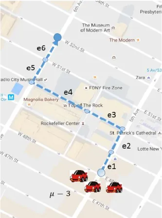
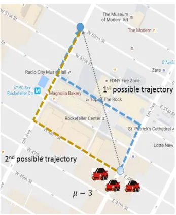
In this thesis, we are more interested in the eventual traffic situation. So instead of studying the trajectory of an individual user, we focus on the overall distribution of trajectories throughout a city level’s road network. Mathematically, we define the trajectory distribution as 𝑡𝑟𝑑 = ((𝑒𝒾1, 𝑒𝒾2, . . , 𝑒𝒾𝑚), 𝜇) , where (𝑒𝒾1, 𝑒𝒾2, . . , 𝑒𝒾𝑚) is a trajectory, while 𝜇 is the estimated number of people or vehicles that would follow this trajectory. Figure 4.1 gives an example of trajectory distribution 𝑡𝑟𝑑 = ((𝑒₁, 𝑒₂, 𝑒₃, 𝑒₄, 𝑒₅, 𝑒₆), 3), which indicates that there are three vehicles that would follow the trajectory (𝑒₁, 𝑒₂, 𝑒₃, 𝑒₄, 𝑒₅, 𝑒₆).

To infer all the trajectory distributions in the road network, there are two specific questions that must be answered:

(1) Given any pair of origin and destination road segment (e.g., 𝑒₁ and 𝑒2) , how many vehicles will travel from segment to another?

(2) What are the probable trajectories that people would follow from the origin road segment to the destination road segment, and what is the corresponding possibility of each trajectory?

We will address these two questions in the next subsections including their challenges, and our proposed solutions.

Figure 4.1: An illustration of a trajectory distribution

4.2 Flow Volume Between Road Segments

The traffic that moves from one road segment to another over a short time period could be sparse, which would make it difficult to directly predict. Because we are more interested in the overall traffic situation in a city level, we could take advantage of the previously predicted flow of traffic between any two neighborhoods. Based on these

predictions, we could further estimate the corresponding flow volume between any two road segments.

In particular, a trip that would head from one neighborhood (e.g., neighborhood 𝑖) to another neighborhood (e.g., neighborhood 𝑗), it could start from any road segment in neighborhood 𝑖 and end in any road segment in neighborhood 𝑗. But in the real world, we might find that some road segments are more popular as origins and some road segments are more popular as destinations during different time periods. For example, a road segment in New York City that includes a large office building such as One World Trade Center, the tallest building in New York with 104 stories and 3 million square feet of office space (WorldTradeCenter 2017), would definitely be a much more popular destination in the morning and origin in the evening, respectively, as compared with other road segments. Given the number of people/vehicles heading from neighborhood 𝑖 to neighborhood 𝑗, in order to estimate how likely they would start from a road segment 𝒾 (in origin neighborhood 𝑖) and end at another road segment 𝒿 (in destination neighborhood 𝑗), we adapt the idea of a spatial interaction gravity model, as proposed by (Wilson 1967). We first estimate the spatial interaction level between any origin road segment 𝒾 (in neighborhood 𝑖) and destination road segment 𝒿 (in neighborhood 𝑗) during time period 𝑙 as:

𝑓( 𝒾, 𝒿, 𝑙) = 𝒢𝑤𝑜𝒾,𝑙×𝑤𝜄𝒿,𝑙

where 𝒢 is a constant parameter, 𝑤_{𝑜𝒾,𝑙} is the weight of road segment 𝒾 as the origin during time period 𝑙, 𝑤_{𝜄𝒿,𝑙} is the corresponding weight of road segment 𝒿 as the destination, and 𝑑𝒾,𝒿 is the Euclidean distance between them. It is worth noting that some previous works use different categories of data to approximate the weight 𝑤. Among all those categories of data, one of the most widely used is the population of corresponding spatial area (Hua and Porell 1979)-but the static population of corresponding area does not work in this scenario. One major reason is that because we focus on the short term prediction, e.g., a city level’s mobility in an hour, while the population feature might be more suitable for some long-term and static prediction. For example, in urban areas, especially those central business districts, people come and go from time to time every day, making it impossible to accurately count or even estimate the population of each area every hour. As a result, we would like to estimate weight 𝑤 based on our history mobility dataset. In particular, in our implementation, we use the historical average number of trips that started from road segment 𝒾 during time period 𝑙 as the weight 𝑤_{𝑜𝒾,𝑙}, and the corresponding historical average number of trips that ended at 𝑒𝒿 as the weight 𝑤_{𝜄𝒿,𝑙}.

Instead of estimating a constant value for 𝒢 like some previous works, we propose to normalize the interaction level between each pair of road segments 𝒾 and 𝒿 in origin neighborhood 𝑖 and destination neighborhood 𝑗, and multiply it by 𝓍_{𝑖,𝑙,𝑗} (the flow volume from neighborhood 𝑖 to neighborhood 𝑗), in order to obtain the flow volume between

those road segments. Eventually, 𝑥𝑒𝒾,𝑙,𝒿, the number of vehicles that are heading from road segment 𝒾 (in neighborhood 𝑖) to road segment 𝒿 (in neighborhood 𝑗) during time period 𝑙 is computed as:

𝓍𝑒_{𝒾,𝑙,𝒿} = 𝓍_{𝑖,𝑙,𝑗} 𝑤𝑜𝒾,𝑙×𝑤𝜄𝒿,𝑙 𝑑𝒾,𝒿 ∑ ∑ 𝑤𝑜𝑝,𝑙×𝑤𝜄𝑞,𝑙 𝑑𝑝,𝑞 𝑞 𝑝 (4.2)

The intuition behind this equation is that if the road segments 𝑒_𝒾 and 𝑒_𝒿 have strong spatial interaction during time period 𝑙 given the historical dataset, a new trip heading from neighborhood 𝑖 to neighborhood 𝑗 will also be likely to start from road segment 𝑒_𝒾 and end at 𝑒_𝒿 then.

4.3 Trajectory Distribution Simulation

After the estimation of flow between road segments in the road work, we turn to our second question: What are the probable trajectories of vehicles heading from one road segment to another and the corresponding possibility of each trajectory?. This problem is also nontrivial, due to the fact that there are usually multiple routes for a vehicle to travel from one place to another in the road network. Figure 4.2 shows an example of the different types of trajectories that can be used to travel from one road segment to another.