Basic Queueing Theory

(1)

Basic Queueing Theory

Dr. János Sztrik

(2)

Reviewers: Dr. József Bíró

Doctor of the Hungarian Academy of Sciences, Full Professor Budapest University of Technology and Economics

Dr. Zalán Heszberger PhD, Associate Professor

(3)

This book is dedicated to my wife without whom this

work could have been finished much earlier.

• If anything can go wrong, it will.

• If you change queues, the one you have left will start to move faster than the one you are in now.

• Your queue always goes the slowest.

• Whatever queue you join, no matter how short it looks, it will always take the longest for you to get served.

(4)

(5)

Exercises

117

4 Infinite-Source Systems 119

(6)

5 Finite-Source Systems 137

III

Queueing Theory Formulas

141

6 Relationships 143

6.1 Notations and Definitions . . . 143

6.2 Relationships between random variables . . . 145

7 Basic Queueing Theory Formulas 147 7.1 M/M/1 Formulas . . . 147 7.2 M/M/1/K Formulas . . . 149 7.3 M/M/c Formulas . . . 150 7.4 M/M/2 Formulas . . . 152 7.5 M/M/c/c Formulas . . . 154 7.6 M/M/c/K Formulas . . . 155 7.7 M/M/∞ Formulas . . . 157 7.8 M/M/1/K/K Formulas . . . 158 7.9 M/G/1/K/K Formulas . . . 160 7.10 M/M/c/K/K Formulas . . . 161 7.11 D/D/c/K/K Formulas . . . 163 7.12 M/G/1 Formulas . . . 164 7.13 GI/M/1 Formulas . . . 173 7.14 GI/M/c Formulas . . . 175

7.15 M/G/1 Priority queueing system . . . 177

7.16 M/G/c Processor Sharing system . . . 185

7.17 M/M/c Priority system . . . 186

(7)

Preface

Modern information technologies require innovations that are based on modeling, ana-lyzing, designing and finally implementing new systems. The whole developing process assumes a well-organized team work of experts including engineers, computer scientists, mathematicians, physicist just to mention some of them. Modern infocommunication networks are one of the most complex systems where the reliability and efficiency of the components play a very important role. For the better understanding of the dynamic behavior of the involved processes one have to deal with constructions of mathematical models which describe the stochastic service of randomly arriving requests. Queueing Theory is one of the most commonly used mathematical tool for the performance evalu-ation of such systems.

The aim of the book is to present the basic methods, approaches in a Markovian level for the analysis of not too complicated systems. The main purpose is to understand how models could be constructed and how to analyze them. It is assumed the reader has been exposed to a first course in probability theory, however in the text I give a refresher and state the most important principles I need later on. My intention is to show what is behind the formulas and how we can derive formulas. It is also essential to know which kind of questions are reasonable and then how to answer them.

My experience and advice are that if it is possible solve the same problem in different ways and compare the results. Sometimes very nice closed-form, analytic solutions are obtained but the main problem is that we cannot compute them for higher values of the involved variables. In this case the algorithmic or asymptotic approaches could be very useful. My intention is to find the balance between the mathematical and practitioner needs. I feel that a satisfactory middle ground has been established for understanding and applying these tools to practical systems. I hope that after understanding this book the reader will be able to create his owns formulas if needed.

It should be underlined that most of the models are based on the assumption that the involved random variables are exponentially distributed and independent of each other. We must confess that this assumption is artificial since in practice the exponential distri-bution is not so frequent. However, the mathematical models based on the memoryless property of the exponential distribution greatly simplifies the solution methods resulting in computable formulas. By using these relatively simple formulas one can easily foresee the effect of a given parameter on the performance measure and hence the trends can be forecast. Clearly, instead of the exponential distribution one can use other distributions but in that case the mathematical models will be much more complicated. The analytic

(8)

results can help us in validating the results obtained by stochastic simulation. This ap-proach is quite general when analytic expressions cannot be expected. In this case not only the model construction but also the statistical analysis of the output is important.

The primary purpose of the book is to show how to create simple models for practical problems that is why the general theory of stochastic processes is omitted. It uses only the most important concepts and sometimes states theorem without proofs, but each time the related references are cited.

I must confess that the style of the following books greatly influenced me, even if they are in different level and more comprehensive than this material: Allen [2], Jain [41], Kleinrock [48], Kobayashi and Mark [51], Stewart [74], Tijms [91], Trivedi [94].

This book is intended not only for students of computer science, engineering, operation research, mathematics but also those who study at business, management and planning departments, too. It covers more than one semester and has been tested by graduate students at Debrecen University over the years. It gives a very detailed analysis of the involved queueing systems by giving density function, distribution function, generating function, Laplace-transform, respectively. Furthermore, Java-applets are provided to cal-culate the main performance measures immediately by using the pdf version of the book in a WWW environment. Of course these applets can be run if one reads the printed version. I have attempted to provide examples for the better understanding and a collection of exercises with detailed solution helps the reader in deepening her/his knowledge. I am convinced that the book covers the basic topics in stochastic modeling of practical problems and it supports students in all over the world.

I am indebted to Professors József Bíró and Zalán Heszberger for their review, com-ments and suggestions which greatly improved the quality of the book. I am also very grateful to Tamás Török, Zoltán Nagy and Ferenc Veres for their help in editing. .

All comments and suggestions are welcome at:

[email protected]

http://irh.inf.unideb.hu/user/jsztrik

Debrecen, 2012.

(9)

Part I

(10)

(11)

Chapter 1

Fundamental Concepts of Queueing

Theory

Queueing theory deals with one of the most unpleasant experiences of life, waiting. Queue-ing is quite common in many fields, for example, in telephone exchange, in a supermarket, at a petrol station, at computer systems, etc. I have mentioned the telephone exchange first because the first problems of queueing theory was raised by calls and Erlang was the first who treated congestion problems in the beginning of 20th century, see Erlang [21, 22].

His works inspired engineers, mathematicians to deal with queueing problems using probabilistic methods. Queueing theory became a field of applied probability and many of its results have been used in operations research, computer science, telecommunication, traffic engineering, reliability theory, just to mention some. It should be emphasized that is a living branch of science where the experts publish a lot of papers and books. The easiest way is to verify this statement one should use the Google Scholar for queueing re-lated items. A Queueing Theory Homepage has been created where readers are informed about relevant sources, for example books, softwares, conferences, journals, etc. I highly recommend to visit it at

http://web2.uwindsor.ca/math/hlynka/queue.html

There is only a few books and lectures notes published in Hungarian language, I would mention the work of Györfi and Páli [33], Jereb and Telek [43], Kleinrock [48], Lakatos and Szeidl , Telek [55] and Sztrik [84, 83, 82, 81]. However, it should be noted that the Hungarian engineers and mathematicians have effectively contributed to the research and applications. First of all we have to mention Lajos Takács who wrote his pioneer and fa-mous book about queueing theory [88]. Other researchers are J. Tomkó, M. Arató, L. Györfi, A. Benczúr, L. Lakatos, L. Szeidl, L. Jereb, M. Telek, J. Bíró, T. Do, and J. Sztrik. The Library of Faculty of Informatics, University of Debrecen, Hungary offer a valuable collection of queueing and performance modeling related books in English, and Russian, too. Please visit:

http://irh.inf.unideb.hu/user/jsztrik/education/05/3f.html

I may draw your attention to the books of Takagi [85, 86, 87] where a rich collection of references is provided.

(12)

1.1

Performance Measures of Queueing Systems

To characterize a queueing system we have to identify the probabilistic properties of the incoming flow of requests, service times and service disciplines. The arrival process can be characterized by the distribution of theinterarrival timesof the customers, denoted byA(t), that is

A(t) =P( interarrival time < t).

In queueing theory these interarrival times are usually assumed to be independent and identically distributed random variables. The other random variable is theservice time, sometimes it is called service request, work. Its distribution function is denoted byB(x), that is

B(x) = P( service time < x).

The service times, and interarrival times are commonly supposed to be independent random variables.

The structure of service and service discipline tell us the number of servers, the capacity of the system, that is the maximum number of customers staying in the system including the ones being under service. The service discipline determines the rule according to the next customer is selected. The most commonly used laws are

• FIFO - First In First Out: who comes earlier leaves earlier

• LIFO - Last Come First Out: who comes later leaves earlier

• RS - Random Service: the customer is selected randomly

• Priority.

The aim of all investigations in queueing theory is to get the main performance measures of the system which are the probabilistic properties ( distribution function, density function, mean, variance ) of the following random variables: number of customers in the system, number of waiting customers, utilization of the server/s, response time of a customer, waiting time of a customer, idle time of the server, busy time of a server. Of course, the answers heavily depends on the assumptions concerning the distribution of interarrival times, service times, number of servers, capacity and service discipline. It is quite rare, except for elementary or Markovian systems, that the distributions can be computed. Usually their mean or transforms can be calculated.

For simplicity consider first a single-server system Let %, called traffic intensity, be defined as

%= mean service time mean interarrival time.

Assuming an infinity population system with arrival intensity λ, which is reciprocal of the mean interarrival time, and let the mean service denote by 1/µ. Then we have

%=arrival intensity∗mean service time = λ µ.

(13)

If % > 1 then the systems is overloaded since the requests arrive faster than as the are served. It shows that more server are needed.

Letχ(A) denote the characteristic function of event A, that is χ(A) =

(

1 , if A occurs, 0 , if A does not ,

furthermore let N(t) = 0 denote the event that at time T the server is idle, that is no customer in the system. Then the utilization of the server during time T is defined by 1 T T Z 0 χ(N(t)6= 0)dt ,

where T is a long interval of time. As T → ∞ we get the utilization of the server denoted by Us and the following relations holds with probability 1

Us= lim T→∞ 1 T T Z 0 χ(N(t)6= 0)dt= 1−P0 = Eδ Eδ+Ei,

where P0 is the steady-state probability that the server is idle Eδ, Ei denote the mean

busy period, mean idle period of the server, respectively.

This formula is a special case of the relationship valid for continuous-time Markov chains and proved in Tomkó [93].

Theorem 1 Let X(t) be an ergodic Markov chain, and A is a subset of its state space. Then with probability 1

lim T→∞ 1 T Z T 0 χ(X(t)∈A)dt =X i∈A Pi = m(A) m(A) +m(A),

where m(A) and m(A) denote the mean sojourn time of the chain in A and A during a cycle,respectively. The ergodic ( stationary, steady-state ) distribution of X(t) is denoted by Pi.

In an m-server system the mean number of arrivals to a given server during time T is λT /m given that the arrivals are uniformly distributed over the servers. Thus the utilization of a given server is

Us =

λ mµ.

The other important measure of the system is the throughput of the system which is defined as the mean number of requests serviced during a time unit. In an m-server system the mean number of completed services is m%µ and thus

(14)

However, if we consider now the customers for a tagged customer the waiting and response times are more important than the measures defined above. Let us define by Wj, Tj the waiting, response time of the jth customer, respectively. Clearly the waiting

time is the time a customer spends in the queue waiting for service, and response time is the time a customer spends in the system, that is

Tj =Wj+Sj,

where Sj denotes its service time. Of course, Wj and Tj are random variables and their

mean, denoted by Wj and Tj, are appropriate for measuring the efficiency of the system.

It is not easy in general to obtain their distribution function.

Other characteristic of the system is thequeue length, and the number of customers in the system. Let the random variables Q(t),N(t)denote the number of customers in the queue, in the system at time t, respectively. Clearly, in an m-server system we have

Q(t) = max{0, N(t)−m}.

The primary aim is to get their distributions, but it is not always possible, many times we have only their mean values or their generating function.

1.2

Kendall’s Notation

Before starting the investigations of elementary queueing systems let us introduce a no-tation originated by Kendall to describe a queueing system.

Let us denote a system by

A / B / m / K / n/ D,

where

A: distribution function of the interarrival times, B: distribution function of the service times, m: number of servers,

K: capacity of the system, the maximum number of customers in the system including the one being serviced,

n: population size, number of sources of customers, D: service discipline.

Exponentially distributed random variables are notated by M, meaning Markovain or memoryless.

(15)

FIFO, then they are omitted.

Hence M/M/1 denotes a system with Poisson arrivals, exponentially distributed service times and a single server. M/G/m denotes an m-server system with Poisson arrivals and generally distributed service times.M/M/r/K/nstands for a system where the cus-tomers arrive from a finite-source with n elements where they stay for an exponentially distributed time, the service times are exponentially distributed, the service is carried out according to the request’s arrival by r severs, and the system capacity is K.

1.3

Basic Relations for Birth-Death Processes

Since birth-death processes play a very important role in modeling elementary queueing systems let us consider some useful relationships for them. Clearly, arrivals mean birth and services mean death.

As we have seen earlier the steady-state distribution for birth-death processes can be obtained in a very nice closed-form, that is

(1.1) Pi = λ0· · ·λi−1 µ1· · ·µi P0, i= 1,2,· · · , P0−1 = 1 + ∞ X i=1 λ0· · ·λi−1 µ1· · ·µi .

Let us consider the distributions at the moments of arrivals, departures, respectively, because we shall use them later on.

Let Na, Nd denote the state of the process at the instant of births, deaths, respectively,

and letΠk=P(Na=k), Dk=P(Nd=k), k= 0,1,2, . . . stand for their distributions.

By applying the Bayes’s theorem it is easy to see that

(1.2) Πk = lim h→0 (λkh+o(h))Pk P∞ j=0(λjh+o(h))Pj = P∞λkPk j=0λjPj . Similarly (1.3) Dk= lim h→0 (µk+1h+o(h))Pk+1 P∞ j=1(µjh+o(h))Pj = Pµk∞+1Pk+1 j=1µjPj . Since Pk+1 = λk µk+1 Pk, k = 0,1, . . ., thus (1.4) Dk = λkPk P∞ i=0λiPi = Πk, k = 0,1, . . . .

(16)

In words, the above relation states that the steady-state distributions at the moments of births and deaths are the same. It should be underlined, that it does not mean that it is equal to the steady-state distribution at a random point as we will see later on.

Further essential observation is that in steady-state the mean birth rate is equal to the mean death rate. This can be seen as follows

(1.5) λ = ∞ X i=0 λiPi = ∞ X i=0 µi+1Pi+1 = ∞ X k=1 µkPk =µ.

1.4

Queueing Softwares

To solve practical problems the first step is to identify the appropriate queueing system and then to calculate the performance measures. Of course the level of modeling heavily depends on the assumptions. It is recommended to start with a simple system and then if the results do not fit to the problem continue with a more complicated one. Various software packages help the interested readers in different level. The following links worths a visit

http://web2.uwindsor.ca/math/hlynka/qsoft.html

For practical oriented teaching courses we also have developed a collection of Java-applets calculating the performance measures not only for elementary but for more advanced queueing systems. It is available at

http://irh.inf.unideb.hu/user/jsztrik/education/09/english/index.html

For simulation purposes I recommend

http://www.win.tue.nl/cow/Q2/

If the preprepared systems are not suitable for your problem then you have to create your queueing system and then the creationstarts and the primary aim of the present book is to help this process.

For further readings the interested reader is referred to the following books: Allen [2], Bose [9], Daigle [18], Gnedenko and Kovalenko [31], Gnedenko, Belyayev and Solovyev [29], Gross and Harris [32], Jain [41], Jereb and Telek [43], Kleinrock [48], Kobayashi [50, 51], Kulkarni [54], Nelson [59], Stewart [74], Sztrik [81], Tijms [91], Trivedi [94]. The present book has used some parts of Allen [2], Gross and Harris [32], Kleinrock [48], Kobayashi [50], Sztrik [81], Tijms [91], Trivedi [94].

(17)

Chapter 2

Infinite-Source Queueing Systems

Queueing systems can be classified according to the cardinality of their sources, namely finite-source and infinite-source models. In finite-source models the arrival intensity of the request depends on the state of the system which makes the calculations more com-plicated. In the case of infinite-source models, the arrivals are independent of the number of customers in the system resulting a mathematically tractable model. In queueing net-works each node is a queueing system which can be connected to each other in various way. The main aim of this chapter is to know how these nodes operate.

2.1

The

M/M/

1

Queue

An M/M/1 queueing system is the simplest non-trivial queue where the requests arrive according to a Poisson process with rateλ, that is the interarrival times are independent, exponentially distributed random variables with parameter λ. The service times are also assumed to be independent and exponentially distributed with parameter µ. Further-more, all the involved random variables are supposed to be independent of each other.

Let N(t) denote the number of customers in the system at time t and we shall say that the system is at state k if N(t) = k. Since all the involved random variables are exponentially distributed, consequently they have the memoryless property, N(t) is a continuous-time Markov chain with state space 0,1,· · ·.

In the next step let us investigate the transition probabilities during time h. It is easy to see that Pk,k+1(h) = (λh+o(h)) (1−(µh+o(h)) + + ∞ X k=2 (λh+o(h))k(µh+o(h))k−1, k = 0,1,2, ... .

By using the independence assumption the first term is the probability that during h one customer has arrived and no service has been finished. The summation term is the probability that duringhat least2customers has arrived and at the same time at least1

(18)

has been serviced. It is not difficult to verify the second term iso(h)due to the property of the Poisson process. Thus

Pk,k+1(h) =λh+o(h).

Similarly, the transition probability from statek into state k−1duringhcan be written as Pk,k−1(h) = (µh+o(h)) (1−(λh+o(h)) + + ∞ X k=2 (λh+o(h))k−1(µh+o(h))k =µh+o(h).

Furthermore, for non-neighboring states we have

Pk,j =o(h), |k−j |≥2.

In summary, the introduced random process N(t)is a birth-death process with rates λk =λ, k = 0,1,2, ..., µk =µ, k= 1,2,3....

That is all the birth rates are λ, and all the death rates areµ.

As we notated the system capacity is infinite and the service discipline is FIFO.

To get the steady-state distribution let us substitute these rates into formula (1.1) ob-tained for general birth-death processes. Thus we obtain

Pk =P0 k−1 Y i=0 λ µ =P0 λ µ k , k ≥0.

By using the normalization condition we can see that this geometric sum is convergent iff λ/µ <1 and P0 = 1 + ∞ X k=1 λ µ k!−1 = 1−λ µ = 1−% where %= λ_µ. Thus Pk= (1−%)%k, k = 0,1,2, ...,

which is a modified geometric distribution with success parameter1−%. In the following we calculate the the main performance measures of the system

• Mean number of customers in the system

N = ∞ X k=0 kPk= (1−%)% ∞ X k=1 k%k−1 =

(19)

= (1−%)% ∞ X k=1 d%k d% = (1−%)% d d% 1 1−% = % 1−%. Variance V ar(N) = ∞ X k=0 (k−N)2Pk = ∞ X k=0 k− % 1−% 2 Pk = ∞ X k=0 k2Pk+ % 1−% 2 − ∞ X k=0 2k % 1−%Pk = ∞ X k=0 k(k−1)Pk+ %2 (1−%)2 + % 1−% −2 % 1−% 2 = (1−%)%2 d 2 d%2 ∞ X k=0 %k+ % 1−% − % 1−% 2 = 2% 2 (1−%)2 + % 1−% − % 1−% 2 = % (1−%)2.

• Mean number of waiting customers, mean queue length

Q= ∞ X k=1 (k−1)Pk = ∞ X k=1 kPk− ∞ X k=1 Pk =N−(1−P0) = N −%= %2 1−%. Variance V ar(Q) = ∞ X k=1 (k−1)2Pk−Q 2 = % 2_{(1 +}_%₋_%2₎ (1−%)2 . • Server utilization Us = 1−P0 = λ µ =%. By using Theorem 1 it is easy to see that

P0 = 1 λ 1 λ +Eδ ,

whereEδ ais the mean busy period length of the server, _λ1 is the mean idle time of the server. Since the server is idle until a new request arrives which is exponentially distributed with parameter λ. Hence

1−%= 1 λ 1 λ +Eδ , and thus Eδ= 1 λ % 1−% = 1 λN = 1 µ−λ.

(20)

In the next few lines we show how this performance measure can be obtained in a different way.

To do so we need the following notations.

Let_E(νA),E(νD)denote the mean number of customers that have arrived, departed

during the mean busy period of the server, respectively. Furthermore, let _E(νS)

denote the mean number of customers that have arrived during a mean service time. Clearly E(νD) =E(δ)µ, E(νS) = λ µ, E(νA) =E(δ)λ, E(νA) + 1 =E(νD),

and thus after substitution we get

E(δ) = 1 µ−λ. Consequently E(νD) =E(δ)µ= 1 1−% E(νA) =E(νS)E(νD) = λ µ 1 1−% = % 1−% E(νA) =E(δ)λ= % 1−%.

• Distribution of the response time of a customer

Before investigating the response we show that in any queueing system where the arrivals are Poisson distributed

Pk(t) = Πk(t),

where Pk(t) denotes the probability that at time t the system is a in state k, and

Πk(t)denotes the probability that an arriving customers find the system in state k

at timet. Let

A(t, t+ ∆t)

denote the event that an arrival occurs in the interval (t, t+ ∆t). Then Πk(t) := lim

∆t→0P (N(t) = k|A(t, t+ ∆t)),

Applying the definition of the conditional probability we have Πk(t) = lim

∆t→0

P (N(t) = k ,A(t, t+ ∆t)) P(A(t, t+ ∆t)) =

(21)

= lim

∆t→0

P (A(t, t+ ∆t)|N(t) =k)P (N(t) =k) P(A(t, t+ ∆t)) .

However, in the case of a Poisson process event A(t, t+ ∆t) does not depends on the number of customers in the system at timet and even the time tis irrespective thus we obtain

P (A(t, t+ ∆t)|N(t) =k) =P (A(t, t+ ∆t)), hence for birth-death processes we have

Πk(t) = P (N(t) =k).

That is the probability that an arriving customer find the system in statek is equal to the probability that the system is in state k.

In stationary case applying formula (1.2) with substitutions λi =λ, i = 0,1, . . .

we have the same result.

If a customer arrives it finds the server idle with probability P0 hence the waiting

time is 0. Assume, upon arrival a tagged customer, the system is in state n. This means that the request has to wait until the residual service time of the customer being serviced plus the service times of the customers in the queue. As we assumed the service is carried out according to the arrivals of the requests. Since the ser-vice times are exponentially distributed the remaining serser-vice time has the same distribution as the original service time. Hence the waiting time of the tagged cus-tomer is Erlang distributed with parameters(n, µ)and the response time is Erlang distributed with (n+ 1, µ). Just to remind you the density function of an Erlang distribution with parameters(n, µ) is

fn(x) =

µ(µx)n−1

(n−1)! e

−µx_, _x_≥_0.

Hence applying the theorem of total probability for the density function of the response time we have

fT(x) = ∞ X n=0 (1−%)%n(µx) n n! µe −µx₌_µ(1₋_%)e−µx ∞ X n=0 (%µx)n n! = =µ(1−%)e−µ(1−%)x.

Its distribution function is

FT(x) = 1−e−µ(1−%)x.

That is the response time is exponentially distributed with parameter µ(1−%) =µ−λ.

Hence the expectation and variance of the response time are

T = 1 µ(1−%), V ar(T) = ( 1 µ(1−%)) 2 .

(22)

Furthermore

T = 1

µ(1−%) = 1

µ−λ =Eδ.

• Distribution of the waiting time

Let fW(x) denote the density function of the waiting time. Similarly to the above

considerations for x >0we have fW(x) = ∞ X n=1 (µx)n−1 (n−1)!µe −µx_%n₍₁₋_{%) = (1}₋_%)%µ ∞ X k=0 (µx%)k k! e −µx₌ = (1−%)%µe−µ(1−%)x. Thus fW(0) = 1−%, if x= 0, fW(x) =%(1−%)µe−µ(1−%)x, if x >0. Hence FW(x) = 1−%+% 1−e−µ(1−%)x = 1−%e−µ(1−%)x. The mean waiting time is

W = ∞ Z 0 xfW(x)dx= % µ(1−%) =%Eδ =N 1 µ. Since T =W +S, in additionW and S are independent we get

V ar(T) = 1 (µ(1−ρ))2 =V ar(W) + 1 µ2, thus V ar(W) = 1 (µ(1−ρ))2 − 1 µ2 = 2ρ−ρ2 (µ(1−ρ))2 =ρ 2 (µ(1−ρ))2 − ρ2 (µ(1−ρ))2, that is exactly _E(W2₎₋₍ EW)2. Notice that (2.1) λT =λ 1 µ(1−%) = % 1−% =N . Furthermore (2.2) λW =λ % µ(1−%) = %2 1−% =Q.

Relations (2.1), (2.2) are called Little formulas or Little theorem, or Little law which remain valid under more general conditions.

(23)

Let us examine the states of anM/M/1system at the departure instants of the customers. Our aim is to calculate the distribution of the departure times of the customers. As it was proved in (1.3) at departures the distribution is

Dk =

λkPk

P∞

i=0λiPi

.

In the case of Poisson arrivals λk =λ, k = 0,1, . . ., henceDk=Pk.

Now we are able to calculate the Laplace-transform of the interdeparture time d. Condi-tioning on the state of the server at the departure instants, by using the theorem of total Laplace-transform we have Ld(s) =% µ µ+s + (1−%) λ λ+s µ µ+s,

since if the server is idle for the next departure a request should arrive first. Hence Ld(s) = µ%(λ+s) + (1−%)λµ (λ+s)(µ+s) = λµ%+λs+λµ−λµ% (λ+s)(µ+s) = λ(s+µ) (λ+s)(µ+s) = λ λ+s,

which shows that the distribution is exponential with parameterλand not with µas one might expect. The independence follows from the memoryless property of the exponential distributions and from their independence. This means that the departure process is a Poisson process with rate λ.

This observation is very important to investigate tandem queues, that is when several simple M/M/1 queueing systems as nodes are connected in serial to each other. Thus at each node the arrival process is a Poisson process with parameter λ and the nodes operate independently of each other. Hence if the service times have parameter µi at

the ith node then introducing traffic intensity %i =

λ µi

all the performance measures for a given node could be calculated. Consequently, the mean number of customers in tha network is the sum of the mean number of customers in the nodes. Similarly, the mean waiting and response times for the network can be calculated as the sum of the related measures in the nodes.

Now, let us show how the density function d can be obtained directly without using tha Laplace-transforms. By applying the theorem of total probability we have

fd(x) =%µe−µx+ (1−%) λµ λ−µe −µx₊ λµ µ−λe −λx =λe−µx+µ−λ µ λµ µ−λe −λx₋ λµ µ−λe −µx

(24)

Now let us consider anM/G/1 system and we are interested in under which service time distribution the interdeparture time is exponentially distributed with parameterλ. First prove that the utilization of the system is US =% = λE(S). As it is understandable for

any stationary stable G/G/1 queueing system the mean number of departures during the mean busy period length of the server is one more than the mean number of arrivals during the mean busy period length of the server. That is

E(δ) E(S)

= 1 + E(δ)

E(τ)

, where _E(τ) denotes the mean interarrival times. Hence

E(τ) +E(δ) =E(δ)E(τ) E(S) E(δ) = E(τ)E(S) E(τ)−E(S) =E(S) 1 1−%, where %= E(S) E(τ). Clearly US = E (δ) E(τ) +E(δ) = E(S)₁−1% E(τ) + E₁(−S%) = % 1−% 1 + ₁₋%_% =% <1.

Thus the utilization for anM/G/1system is%. It should be noted that anM/G/1system Dk=Pk, that is why our question can be formulated as

λ λ+s =%LS(s) + (1−%) λ λ+sLS(s) =LS(s) %+λ(1−%) λ+s =LS(s) λ2_E(S) +sλ_E(S) +λ−λ2_E(S) λ+s =LS(s) λ(1 +s_E(S)) λ+s , thus LS(s) = 1 1 +s_E(S),

which is the Laplace-transform of an exponential distribution with mean _E(S). In sum-mary, only exponentially distributed service times assures that Poisson arrivals involves Poisson departures with the same parameters.

Java applets for direct calculationscan be found at

http://irh.inf.unideb.hu/user/jsztrik/education/03/EN/MM1/MM1.html

Example 1 Let us consider a small post office in a village where on the average 70 customers arrive according to a Poisson process during a day. Let us assume that the service times are exponentially distributed with rate 10 clients per hour and the office operates 10 hours daily. Find the mean queue length, and the probability that the number of waiting customer is greater than 2. What is the mean waiting time and the probability that the waiting time is greater than 20 minutes ?

(25)

Solution:

Let the time unit be an hour. Then λ= 7, µ= 10, ρ= ₁₀7

N = ρ 1−ρ = 7 3 Q=N −ρ= 7 3 − 7 10 = 70−21 30 = 49 30 P(n >3) = 1−P(n ≤3) = 1−P0−P1−P2 −P3 = 1−1 +ρ−(1−ρ)(ρ+ρ2+ρ3) =ρ4 = 0.343·0.7 = 0.2401 W = N µ = 7 3·10 = 7 30 hour ≈14 minutes P W > 1 3 = 1−FW 1 3 = 0.7·e−10·13·0.3 = 0.7·e−1 = 0.257

2.2

The

M/M/

1

Queue with Balking Customers

Let us consider a modification of an M/M/1 system in which customers are discouraged when more and more requests are present at their arrivals. Let us denote by bk the

probability that a customers joints to the systems provided there are k customers in the system at the moment of his arrival.

It is easy to see, that the number of customers in the system is a birth-death process with birth rates

λk =λ·bk, k = 0,1, . . .

Clearly, there are various candidates for bk but we have to find such probabilities which

result not too complicated formulas for the main performance measures. Keeping in mind this criteria let us consider the following

bk = 1 k+ 1, k = 0,1, . . . Thus Pk = ρk k!P0, k = 0,1, . . . , and then using the normalization condition we get

Pk=

ρk k!e

−ρ

, k = 0,1, . . .

The stability condition is E ρ < ∞, that is we do not need the condition ρ <1 as in an M/M/1 system.

Notice that the number of customers follows a Poisson law with parameter ρand we can expect that the performnace measures can be obtained in a simple way.

(26)

• US = 1−P0 = 1−e−ρ, US = E (δ) 1 λ +E(δ) , hence E(δ) = 1 λ · US 1−US = 1 λ · 1−e−ρ e−ρ . • N =ρ, V ar(N) = ρ • Q=N −US =ρ−(1−e−ρ) =ρ+e−ρ−1. E(Q2) = ∞ X k=1 (k−1)2Pk = ∞ X k=1 k2Pk−2 ∞ X k=1 kPk+ ∞ X k=1 Pk =_E(N2)−2N +US =ρ+ρ2−2ρ+US =ρ2−ρ+ 1−e−ρ. Thus V ar(Q) =_E(Q2)−(_E(Q))2 =ρ2−ρ+ 1−e−ρ−(ρ+e−ρ−1)2 =ρ2−ρ+ 1−e−ρ−ρ2−e−2ρ−1−2ρe−ρ+ 2ρ+ 2e−ρ =ρ−e−2ρ+e−ρ−2ρe−ρ=ρ−e−ρ(e−ρ+ 2ρ−1).

• To get the distribution of the response and waiting times we have to know the distribution of the system at the instant when an arriving customer joins to the system.

By applying the Bayes’s rule it is not difficult to see that Πk = λ k+1 ·Pk ∞ X i=0 λ i+ 1 ·Pi = ρk+1 (k+1)!·e −ρ ∞ X i=0 ρi+1 (i+ 1)!e −ρ = Pk+1 1−e−ρ.

Notice, that this time

Πk 6=Pk.

Let us first determine T and then W. By the law of total expectations we have

T = ∞ X k=0 k+ 1 µ Πk = 1 µ ∞ X k=0 (k+ 1)Pk+1 1−e−ρ = 1 µ(1−e−ρ₎ ·N = ρ µ(1−e−ρ₎. W =T − 1 µ = 1 µ ρ+e−ρ₋₁ 1−e−ρ .

(27)

As we have proved in formula (1.5) λ = ∞ X k=0 λkPk = ∞ X k=1 µkPk = ∞ X k=1 µPk =µ(1−e−ρ), thus λ·T =µ(1−e−ρ)· ρ µ(1−e−ρ₎ =ρ=N , λ·W =µ(1−e−ρ)· ρ+e −ρ₋₁ µ(1−e−ρ₎ =ρ+e −ρ₋ 1 =Q which is the Little formula for this system.

• To find the distribution of T and W we have to use the same approach as we did earlier, namely fT(x) = ∞ X k=0 fT(x|k)·Πk = ∞ X k=0 µ(µx)k_e−µx k! · ρk+1 (k+ 1)! e−ρ 1−e−ρ = λe −(ρ+µx) 1−e−ρ ∞ X k=0 (µxρ)k k!(k+ 1)!,

which is difficult to calculate. We have the same problems with fW(x), too.

However, the Laplace-transforms LT(s) and LW(s) can be obtained and the hence

the higher moments can be derived. Namely LT(s) = ∞ X k=0 LT(s|k)Πk = ∞ X k=0 µ µ+s k+1 ρ k+1 (k+1)!e −ρ 1−e−ρ = e −ρ 1−e−ρ ∞ X k=0 µρ µ+s k+1 1 (k+ 1)! = e−ρ 1−e−ρ eµµρ+s −₁ . LW(s) =LT(s)· µ+s µ .

Find T by the help of LT(s)to check the formula. It is easy to see that

L0_T(s) = e −ρ 1−e−ρ ·e µρ µ+s(−µρ(µ+s)−2) L0_T(0) =− e −ρ 1−e−ρe ρ_· ρ µ =− ρ µ(1−e−ρ₎. Hence T = ρ µ(1−e−ρ₎,

(28)

as we have obtained earlier.W can be verified similarly.

To getV ar(T)andV ar(W)we can use the Laplace-transform method. As we have seen LT(s) = e−ρ 1−e−ρ eµλ+s −₁ . Thus L0_T(s) = e −ρ 1−e−ρ ·e λ µ+s₍−_1)λ(µ₊_s)−2_, therefore L00_T(s) = e −ρ 1−e−ρ · eµλ+s (−1)λ(µ+s)−22+ 2λ(µ+s)−3·e λ µ+s . Hence L00_T(0) = e −ρ 1−e−ρ e ρ −ρ µ 2 + 2ρ µ2e ρ ! = 1 µ2 · ρ2_{+ 2ρ} 1−e−ρ. Consequently V ar(T) = 1 µ2 · ρ2_{+ 2ρ} 1−e−ρ − ρ µ(1−e−ρ₎ 2 = (ρ 2_{+ 2ρ) (1}₋_e−ρ₎₋_ρ2 µ2₍₁₋_e−ρ₎2 = ρ2+ 2ρ−ρ2e−ρ−2ρe−ρ−ρ2 µ2₍₁₋_e−ρ₎2 = 2ρ−ρ 2_e−ρ₋_2ρe−ρ µ2₍₁₋_e−ρ₎2 = ρ(2−(ρ+ 2)e−ρ₎ µ2₍₁₋_e−ρ₎2 .

However,W and T can be considered as a random sum, too. That is V ar(W) =_E(Na) 1 µ2 +V ar(Na) 1 µ 2 = 1 µ2(E(Na) +V ar(Na)). E(Na) = ∞ X k=1 kΠk= ∞ X k=1 kPk+1 1−e−ρ = 1 1−e−ρ ∞ X k=0 (k+ 1)Pk+1− ∞ X k=0 Pk+1 ! = 1 1−e−ρ ρ+e −ρ₋₁ . Since V ar(Na) =E(Na2)−(E(Na))2

(29)

first we have to calculate _E(N2 a), that is E(Na2) = ∞ X k=1 k2Πk= ∞ X k=1 k2 Pk+1 1−e−ρ = 1 1−e−ρ ∞ X k=0 (k+ 1)2−2k−1Pk+1 = 1 1−e−ρ ∞ X k=0 (k+ 1)2Pk+1−2 ∞ X k=0 kPk+1− ∞ X k=0 Pk+1 ! = 1 1−e−ρ ρ+ρ 2₋ 2 ρ+e−ρ−1− 1−e−ρ = 1 1−e−ρ ρ 2₋_ρ₋_e−ρ_{+ 1} . Therefore V ar(Na) = 1 1−e−ρ ρ 2₋_ρ₋_e−ρ_{+ 1} − 1 1−e−ρ(ρ+e −ρ₋₁₎ 2 = 1 1−e−ρ 2 (1−e−ρ) ρ2−ρ−e−ρ+ 1− ρ+e−ρ−12 = 1 1−e−ρ 2 (ρ2−ρ−e−ρ+ 1−ρ2e−ρ+ρe−ρ+e−2ρ−e−ρ −ρ2−e−2ρ−1−2ρe−ρ+ 2ρ−2e−ρ) = ρ−e −ρ_(ρ2₊_ρ) (1−e−ρ₎2 . Finally V ar(W) = 1 µ 2 1 1−e−ρ(ρ+e −ρ₋ 1) + ρ−e −ρ_(ρ2₊_ρ) (1−e−ρ₎2 = 1 (µ(1−e−ρ₎₎2((ρ+e −ρ₋₁₎₍₁₋_e−ρ_{) +}_ρ₋_e−ρ_(ρ2₊_ρ)). Thus V ar(T) =V ar(W) + 1 µ2 V ar(T) = 1 µ(1−e−ρ₎ 2 (ρ+e−ρ−1)(1−e−ρ) +ρ−e−ρ(ρ2+ρ) + (1−e−ρ)2) = (1−e −ρ_)(ρ₊_e−ρ₋_{1 + 1}₋_e−ρ_{) +}_ρ₋_e−ρ_(ρ2 ₊_ρ) (µ(1−e−ρ₎₎2 = 2ρ−2ρe −ρ₋_ρ2_e−ρ (µ(1−e−ρ₎2

(30)

2.3

Priority

M/M/

1

Queues

In the following let us consider an M/M/1 systems with priorities. This means that we have two classes of customers. Each type of requests arrive according to a Poisson process with parameterλ1, andλ2, respectively and the processes are supposed to be independent

of each other. The service times for each class are assumed to be exponentially distributed with parameter µ. The system is stable if

ρ1+ρ2 <1,

where ρi =λi/µ, i= 1,2.

Let us assume that class 1 has priority over class 2. This section is devoted to the investi-gation of preemptive and non-preemptive systems and some mean values are calculated.

Preemptive Priority

According to the discipline the service of a customer belonging to class2 is never carried out if there is customer belonging to class 1 in the system. In other words it means that class1preempts class2that is if a class2customer is under service when a class1request arrives the service stops and the service of class1 request starts. The interrupted service is continued only if there is no class 1 customer in the system.

Let Ni denote the number of class i customers in the system and let Ti stand for the

response time of class i requests. Our aim is to calculate _E(Ni) and E(Ti) for i = 1,2.

Since type 1 always preempts type 2 the service of class 1 customers is independent of the number of class 2 customers. Thus we have

(2.3) _E(T1) = 1/µ 1−ρ1 , _E(N1) = ρ1 1−ρ1 .

Since for all customers the service time is exponentially distributed with the same pa-rameter, the number of customers does not depends on the order of service. Hence for the total number of customers in an M/M/1 we get

(2.4) _E(N1) +E(N2) =

ρ1+ρ2

1−ρ1−ρ2

, and then inserting (2.3) we obtain

E(N2) = ρ1 +ρ2 1−ρ1−ρ2 − ρ1 1−ρ1 = ρ2 (1−ρ1)(1−ρ1−ρ2) , and using the Little’s law we have

E(T2) = E (N2) λ2 = 1/µ (1−ρ1)(1−ρ1−ρ2) .

Example 2 Let us compare what is the difference if preemptive priority discipline is ap-plied instead of FIFO.

(31)

Let λ1 = 0.5, λ2 = 0.25 and µ= 1. In FIFO case we get

E(T) = 4.0, E(W) = 3.0, E(N) = 3.0

and in priority case we obtain

E(T1) = 2.0, E(W1) = 1.0, E(N1) = 1.0

E(T2) = 8.0, E(W2) = 6.0, E(N2) = 2.0

Non-preemptive Priority

The only difference between the two disciplines is that in the case the arrival of a class 1 customer does not interrupt the service of type2 request. That is why sometimes this discipline is call HOL ( Head Of the Line ). Of course after finishing the service of class 1 starts.

By using the law of total expectations the mean response time for class1can be obtained as E(T1) =E(N1) 1 µ+ 1 µ +ρ2 1 µ.

The last term shows the situation when an arriving class 1 customer find the server busy servicing a class 2customer. Since the service time is exponentially distributed the residual service time has the same distribution as the original one. Furthermore, because of the Poisson arrivals the distribution at arrival moments is the same as at random moments, that is the probability that the server is busy with class 2 customer is ρ2. By

using the Little’s law

E(N1) =λ1E(T1),

after substitution we get

E(T1) = (1 +ρ2)/µ 1−ρ1 , _E(N1) = (1 +ρ2)ρ1 1−ρ1 .

To get the means for class 2 the same procedure can be performed as in the previous case. That is using (2.4) after substitution we obtain

E(N2) =

(1−ρ1(1−ρ1−ρ2))ρ2

(1−ρ1)(1−ρ1−ρ2)

, and then applying the Little’s law we have

E(T2) =

(1−ρ1(1−ρ1−ρ2))/µ

(1−ρ1)(1−ρ1−ρ2)

(32)

Example 3 Now let us compare the difference between the two priority disciplines. Let λ1 = 0.5, λ2 = 0.25 and µ= 1, then

E(T1) = 2.5, E(W1) = 1.5, E(N1) = 1.25

E(T2) = 7.0, E(W2) = 6.0, E(N2) = 1.75

Of course knowing the mean response time and mean number of customers in the system the mean waiting time and the mean number of waiting customers can be obtained in the usual way.

http://irh.inf.unideb.hu/user/jsztrik/education/03/EN/MMcPrio/MMcPrio.html http://www.win.tue.nl/cow/Q2/

2.4

The

M/M/

1

/K

Queue, Systems with Finite

Capac-ity

LetK be the capacity of anM/M/1system, that is the maximum number of customers in the system including the one under service. It is easy to see that the nu,ber of customers in the systems is a birth-death process with rates λk = λ, k = 0, . . . , K −1 és µk =µ,

k = 1, . . . , K. For the steady-state distribution we have Pk = ρk K X i=0 ρi , k= 0, . . . , K, that is P0 = 1 K X i=0 ρi =      1 K+1, ρ= 1 1−ρ 1−ρK+1, ρ6= 1.

It sholud be noted that the system is stable for any ρ > 0 when K is fixed. However, if K → ∞the the stability condition isρ <1since the distribution ofM/M/1/Kconverges to the distribution ofM/M/1.

It can be verified analytically since ρK _→₀ _then _P

0 →1−ρ.

Similarly to anM/M/1systems after reasonable modifications theperformance measures can be computed as • US = 1−P0, E(δ) = 1 λ US 1−US

(33)

• N = K X k=1 kρkP0 =ρP0 K X k=1 kρk−1 =ρP0 K X k=1 ρk !0 =ρP0 ρ1−ρ K 1−ρ 0 =ρP0 ρ−ρK+1 1−ρ 0 = 1−(K+ 1)ρK(1−ρ) +ρ−ρK+1· ρP0 (1−ρ)2 = ρP0 1−(K+ 1)ρ K ₋_ρ_{+ (K}_{+ 1)ρ}K+1₊_ρ₋_ρK+1 (1−ρ)2 = ρP0 1−(K+ 1)ρ K ₊_KρK+1 (1−ρ)2 = ρ 1−(K + 1)ρ K₊_KρK+1 (1−ρ)(1−ρK+1₎ . • Q= K X k=1 (k−1)Pk= K X k=1 kPk− K X k=1 Pk=N −US

• To obtain the distribution of the response and waiting time we have to know the distribution of the system at the moment when the tagged customer enters into to system. It should be underlined that the customer should enter into the system and it is not the same as an arriving customer. An arriving customer can join the system or can be lost because the system is full. By using the Bayes’ theorem it is easy to see that

Πk= λPk K−1 X i=0 λPi = Pk 1−PK .

Similarly to the investigations we carried out in an M/M/1 system the mean and the density function of the response time can be obtained by the help of the law of total means and law of total probability, respectively.

For the expectation we have

T = K−1 X k=0 k+ 1 µ Πk= K−1 X k=0 k+ 1 µ ρk_P 0 1−Pk = 1 λ(1−PK) K−1 X k=0 (k+ 1)Pk+1 = N λ(1−PK) .

(34)

Consequently W =T − 1 µ = N λ(1−PK) − 1 µ.

We would like to show that the Little’s law is valid in this case and the same time we can check the correctness of the formula.

It can easily be seen that the average arrival rate into the system is λ=λ(1−PK)

and thus λ·T =λ(1−PK) N λ(1−PK) =N . Similarly λ·W =λ N λ(1−PK) − 1 µ =N− λ µ =N −ρ(1−PK) = N −US =Q, since λ=µ=µUS.

Now let us find the density function of the response and waiting times By using the theorem of total probability we have

fT(x) = K−1 X k=0 µ(µx) k k! e −µx Pk 1−PK ,

and thus for the distribution function we get

FT(x) = K−1 X k=0   x Z 0 µ(µt) k k! e −µt dt   Pk 1−PK = K−1 X k=0 1− k X i=0 (µx)i i! e −µx ! Pk 1−PK = 1− K−1 X k=0 k X i=0 (µx)i i! e −µx ! Pk 1−PK .

Thes formulas are more complicated due to the finite summation as in the case of anM/M/1system, but it is not difficult to see that in the limiting case as K → ∞

we have

(35)

For the density and distribution function of the waiting time we obtain fW(0) = P0 1−PK fW(x) = K−1 X k=1 µ(µx) k−1 (k−1)!e −µx Pk 1−PK , x >0 FW(x) = P0 1−PK + K−1 X k=1 1− k−1 X i=0 (µx)i i! e −µx ! Pk 1−PK = 1− K−1 X k=1 k−1 X i=0 (µx)i i! e −µx ! · Pk 1−PK . These formulas can be calculated very easily by a computer.

As we can see the probability PK plays an important role in the calculations.

Notice that it is exactly the probability that an arriving customer find the system full that is it lost. It is calledblocking or lost probability and denoted by PB.

Its correctness can be proved by the help of the Bayes’s rule, namely PB = λPK K X k=0 λPk =PK.

If we would like to show the dependence onK and ρit can be denoted by PB(K, ρ) = ρK K X k=0 ρk . Notice that PB(K, ρ) = ρρK−1 K−1 X k=0 ρk+ρρK−1 = ρPB(K−1, ρ) 1 +ρPB(K−1, ρ) .

Starting with the initial value PB(1, ρ) =

ρ

1 +ρ the probability of loss can be com-puted recursively. It is obvious that this sequence tends to0asρ <1. Consequently by using the recursion we can always find anK-t, for which

PB(K, ρ)< P∗,

where P∗ is a predefined limit value for the probability of loss.

To find the value ofK without recursion we have to solve the inequality ρK(1−ρ)

1−ρK+1 < P

(36)

which is more complicated task.

Alternatively can can find an approximation method, too. Use the distribution of anM/M/1 system and find the probability that in the system there are at leastK customers. It is easy to see that

PB(K, ρ) = ρK₍₁₋_ρ) 1−ρK+1 < ∞ X k=K ρk(1−ρ) = ρK, and thus if ρK < P∗, then P_B∗(K, ρ)< P∗. That is Klnρ <lnP∗ K > lnP ∗ lnρ .

Now let us turn our attention to the Laplace-transform of the response and wait-ing times. First let us compute it for the response time. Similarly to the previous arguments we have LT(s) = K−1 X k=0 µ µ+s k+1 ρk_P 0 1−PK = P0 ρ(1−PK) K X l=1 µρ µ+s l = P0 ρ(1−PK) λ µ+s 1− λ µ+s K 1− λ µ+s = µP0 (1−PK) 1− λ µ+s K µ−λ+s .

The Laplace-transform of the waiting time can be obtained as LW(s) = K−1 X k=0 µ µ+s k ρkP0 1−PK = P0 1−PK K−1 X k=0 µρ µ+s k = P0 1−PK 1− λ µ+s K 1− λ µ+s = P0 1−PK (µ+s) 1− λ µ+s K µ−λ+s ,

(37)

which also follows from relation

LT(s) =LW(s)·

µ µ+s.

By the help of the Laplace-transforms the higher moments of the involved random variables can be computed, too.

http://irh.inf.unideb.hu/user/jsztrik/education/03/EN/MM1K/MM1K.html

2.5

The

M/M/

∞

Queue

Similarly to the previous systems it is easy to see that the number of customers in the system, that is the process (N(t), t≥0) is a birth-death process with rates

λk=λ, k= 0,1, . . .

µk=kµ, k= 1,2, . . . .

Hence the steady-state distribution can be obtained as Pk = %k k!P0, where P −1 0 = ∞ X k=0 %k k! =e %_, That is Pk = %k k!e −% , showing that N follows a Poisson law with parameter %.

It is easy to see that theperformance measures can be computed as N =%, λ =λ, T = 1 µ, W = 0, r=N , µ=rµ Ur= 1−e−%, E (δr) 1 λ = 1−e −% e−% , E(δr) = 1 λ 1−e−% e−% .

It can be proved that these formulas remain valid for an M/G/∞ system as well where

E(S) = 1

µ.

(38)

2.6

The

M/M/n/n

Queue, Erlang-Loss System

This system is the oldest and thus the most famous system in queueing theory. The ori-gin of the traffic theory or congestion theory started by the investigation of this system and Erlang was the first who obtained his well-reputed formulas, see for example Erlang [21, 22].

By assumptions customers arrive according to a Poisson process and the service times are exponentially distributed. However, ifn servers all busy when a new customer arrives it will be lost because the system is full. The most important question is what proportion of the customers is lost.

The process(N(t), t≥0)is said to be in statekifkservers are busy, which is the same as k customers are in the system. It is easy to see that (N(t), t≥0)is a birth-death process with rates λk = ( λ, if k < n, 0, if k ≥n, µk =kµ, k = 1,2, ..., n.

Clearly the steady-state distribution exists since the process has a finite state space. The stationary distribution can be obtained as

Pk =      P0 λ µ k 1 k! , if k ≤n, 0 , if k > 0. Due to the normalizing condition we have

P0 = n X k=0 λ µ k 1 k! !−1 , and thus the distribution is

Pk = λ µ k 1 k! n X i=0 λ µ i 1 i! = %k k! n X i=0 %i i! , k ≤n.

The most important measure of the system is

Pn = %n n! n X k=0 %k k! =B(n, ρ)

which was introduced by Erlang and it is referred to as Erlang’s B-formula, or loss formula and generally denoted by B(n, λ/µ).

(39)

By using the Bayes’s rule it is easy to see that Pn is the probability that an arriving

customer is lost. For moderate n the probability P0 can easily be computed. For large n

and small % P0 ≈e−%, and thus

Pk ≈

%k

k!e

−%_,

that is the Poisson distribution. For large n and large %

n X j=0 %j j! 6=e % .

However, in this case the central limit theorem can be used, since the denominator is the sum of the first(n+ 1) terms of a Poisson distribution with mean%. Thus by the central limit theorem this Poisson distribution can be approximated by a normal law with mean % and variance √% that is

Pn ≈ Φ(s)−Φ(s−1/√%) Φ(s) = 1− Φ(s−1/√%) Φ(s) , where Φ(s) = s Z −∞ 1 √ 2πe −x2 2 dx, and s= n+ 1 2 −% √ % .

Another way to calculate B(n, ρ) is to find a recursion. This can be obtained as follows

B(n, p) = ρn n! n X i=0 ρi i! = ρ n ρn−1 (n−1)! n X i=0 ρi i! + ρ n ρn−1 (n−1)! = ρ nB(n−1, ρ) 1 + ρ_nB(n−1, ρ) = ρB(n−1, ρ) n+ρB(n−1, ρ). Using B(1, ρ) = ρ

1 +ρ as an initial value the probabilities B(n, ρ) can be computed for any n. It is important since the direct calculation can cause a problem due to the value of the factorial.

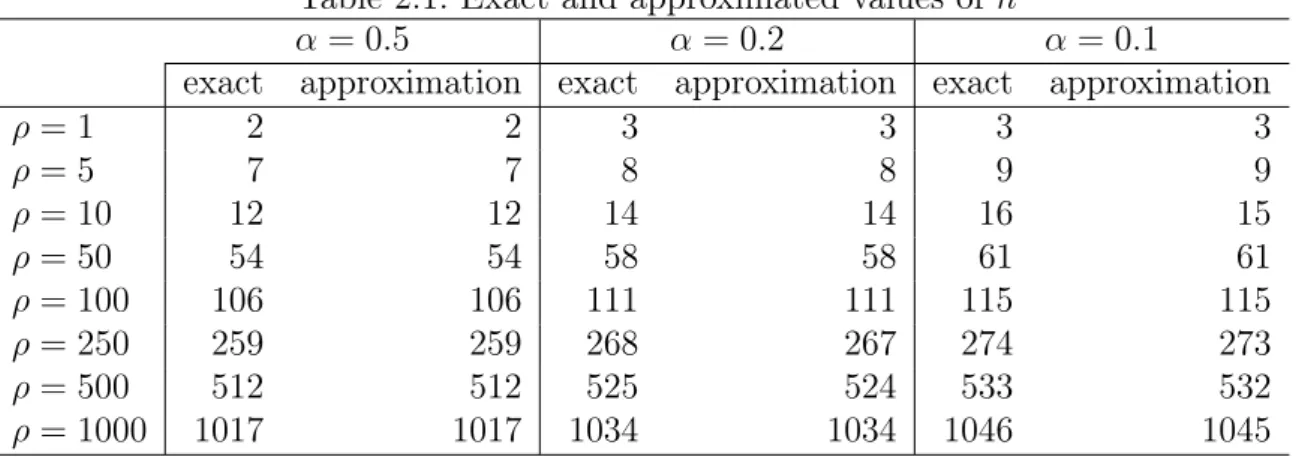
For example for n = 1000, ρ = 1000 the exact formula cannot be computed but the ap-proximation and the recursion gives the value 0.024.

Due to the great importance of B(n, ρ) in practical problems so-called calculators have been developed which can be found at

(40)

To compare the approximations and the exact values we also have developed our own Java script which can be used at

http://jani.uw.hu/erlang/erlang.html

Now determine the main performance measures of this M/M/n/n system

• Mean number of customers in the systems, mean number of busy servers

N =n = n X j=0 jPj = n X j=0 j% j j!P0 =% n−1 X j=0 %i i!P0 =%(1−Pn), thus the mean number of requests for a given server is

% n(1−Pn). • Utilization of a server As we have seen Us = n X i=1 i nPi = ¯ n n. This case Us= % n(1−Pn).

• The mean idle period for a given server By applying the well-known relation

P(the server is idle ) = 1/µ e+ 1/µ, where e is the mean idle time of the server. Thus

% n(1−Pn) = 1/µ e+ 1/µ, hence e= n λ(1−Pn) − 1 µ.

• The mean busy period of the system Clearly Ur = 1−P0 = Eδr 1 λ +Eδr , thus Eδr = 1−P0 λP0 = n X i=1 %i i! λ 1 + n X i=1 %i i! !.

(41)

http://irh.inf.unideb.hu/user/jsztrik/education/03/EN/MMcc/MMcc.html

Example 4 In busy parking lot cars arrive according to a Poisson process one in 20 seconds and stay there in the average of 10minutes.

How many parking places are required if the probability of a loss is no to exceed 1% ? Solution: ρ= λ µ = 10 1 3 = 30, Pn = 0.01.

Following a normal approximation

Pn = 0.01 = ρn n!e −ρ Φ _n₊1 2−ρ √ ρ = Φn+ 1 2−ρ √ ρ −Φn− 1 2−ρ √ ρ Φ _n₊1 2−ρ √ ρ . Thus 0.99Φ _n₊1 2 −ρ √ ρ = Φ _n₋ 1 2 −ρ √ ρ .

It is not difficult to verify by using the Table for the standard normal distribution that n= 41.

Thus the approximation value of P41 is0.009917321712214377,

and the exact value is 0.01043318100246811.

Example 5 A telephone exchange consists of 50 lines and calls arrive according to a Poisson process, the mean interarrival time is 10 minutes. The mean service time is 5 minutes.

Find the main performance measures. Solution:

Using Poisson approximation whereρ= λ_µ = 0.5 P50= 0.00000, event for n = 6

P6 = 0,00001. This means that a call is almost never lost.

Mean number of busy lines can be obtain as

n =ρ(1−Pn) =ρ= 0.5 ,

The utilization of a line is 0.5

50 =

5×10−1

5×10 = 10

−2

The utilization of the system is

(42)

The mean busy period of the system can be obtained as Eδr = (1−P0) (λP0) = 0.394 2×0.606 = 0.394 1.212 = 0.32 minutes Mean idle period of a line is

e= n λ(1−Pn) − ρ λ = 50 2(1−0) − 0,5 2 = 25− 1 4 = 24.75 minutes

Heterogeneous Servers

In the case of an M/−M /n/n→ system the service time distribution depends on the index of the server. That is the service time is exponentially distributed with parameterµi for

server i. An arriving customer choose randomly among the idle servers, that is each idle server is chosen with the same probability. Since the servers are heterogeneous it is not enough to to the number of busy servers but we have to identify them by their index. It means that we have to deal with general Markov-processes.

Let (i1, . . . , ik) denote the indexes of the busy servers, which are the combinations of n

objects takenk at a time without replacement. Thus the state space of the Markov-chain is the set of these combinations, that is (0,(i1, . . . , ik)∈Ckn, k = 1, . . . , n).

Let us denote by

P0 =P(0),

P(i1, . . . , ik) = P((i1, . . . , ik)),(i1, . . . , ik)∈Ckn, k = 1, . . . , n

the steady-state distribution of the chain which exists since the chain has a finite state space and it is irreducible. The set of steady-state balance equations can be written as

(2.5) λP0 = n X j=1 µjP(j) (λ+ k X j=1 µij)P(i1, . . . , ik) = λ n−k+ 1 k X j=1 P(i1, . . . , ij−1, ij+1, . . . , ik) + X j6=i1,...,ik µjP(i01, . . . , i 0 k, j 0₎ (2.6) (2.7) n X j=1 µj P(1, . . . , n) =λ n X j=1 P(1, . . . , j−1, j+ 1, . . . , n)

(43)

where (i0₁, . . . , i0_k, j0) denotes the ordered set i1, . . . , ik, j, i−1 and in+1 are not defined.

Despite of the large number of unknowns, which is2n_{, the solution is quite simple, namely}

(2.8) P(i1, . . . , ik) = (n−k)! k Y j=1 %ijC, where %j = λ µi

, j = 1, . . . , n, P0 =n!C, which can be determined by the help of the

normalizing condition P0+ n X k=1 X (i1,...,ik)∈Ckn P(i1, . . . , ik) = 1.

Let us check the first equation (2.5). By substitution we have λn!C = n X j=1 µj λ µj (n−1)!C =n!λC.

Lets us check now the third equation (2.7)

n X j=1 µj λn µ1· · ·µn C=λ n X j=1 λn−1C µ1· · ·µj−1µj+1· · ·µn = λ n µ1· · ·µn n X j=1 µj C.

Finally let us check the most complicated one, the second set of equations (2.6), namely

(λ+ k X j=1 µij)(n−k)! k Y j=1 %ijC = λ n−k+ 1(n−k+ 1)! k X j=1 λk−1C µi1· · ·µij−1µij+1· · ·µik + X j6=i1,...,ik (n−k−1)! λ k+1_µ jC µi1· · ·µikµj = (n−k)! k X j=1 µijλ k_C µi1· · ·µik +λ X j6=i1,...,ik (n−k−1)! λ k_C µi1· · ·µik = (n−k)! k X j=1 µij λk_C µi1· · ·µik +λ(n−k)! λ k_C µi1· · ·µik ,

which shows the equality.

(44)

• the utilization of the jth server Uj can be calculated as Uj = n X k=1 X j∈(i1,...,ik) P(i1, . . . , ik), and thus Uj = 1 µj 1 µj +E(ej) ,

where _E(ej) is the mean idle period of thejth server. Hence

E(ej) = 1 µj 1−Uj Uj . • N =Pn j=1Uj

• The probability of loss is PB =P(1, . . . , n).

It should be noted that in this case the following relation also holds λ(1−PB) =

n

X

j=1

Ujµj.

In homogeneous case, that is when µj =µ, j= 1, . . . , n, after substitution we have

Pk= X (i1,...,ik)∈Cnk P(i1, . . . , ik) = n k (n−k)!%kC= % k k!n!C = %k k!P0 = %k k! Pn j=1 %j j! ,

that is it reduces to the Erlang’s formula derived earlier.

It should be noted that these formulas remains valid under generally distributed service times with finite means with ρi = λE(Si). In other words the Erlang’s loss formula is

robust to the distribution of the service time, it does not depend on the distribution itself but only on its mean.

2.7

The

M/M/n

Queue

It is a variation of the classical queue assuming that the service is provided by n servers operating independently of each other. This modification is natural since if the mean arrival rate is greater than the service rate the system will not be stable, that is why the number of servers should be increased. However, in this situation we have parallel services and we are interested in the distribution of first service completion.

(45)

Let Xi be exponentially distributed random variables with parameter µi, (i = 1,2, ..., r)

and denote by Y their minimum. It is not difficult to see that Y is also exponentially distributed with parameter

r P i=1 µi since P(Y < x) = 1−P(Y ≥x) = 1−P(Xi ≥x, i= 1, ..., r) = = 1− r Y i=1 P(Xi ≥x) = 1−e−( Pr i=1µi)x_.

Similarly to the earlier investigations, it can easily be verified that the number of cus-tomers in the system is a birth-death process with the following transition probabilities

Pk,k−1(h) = (1−(λh+o(h))) (µkh+o(h)) +o(h) = µkh+o(h),

Pk,k+1(h) = (λh+o(h)) (1−(µkh+o(h))) +o(h) = λh+o(h),

where µk = min(kµ, nµ) =      kµ , for 0≤k ≤n, nµ , for n < k. It is understandable that the stability condition is λ/nµ <1.

To obtain the distributionPk we have to distinguish two cases according to asµk depends

onk. Thus if k < n, then we get Pk=P0 k−1 Y i=0 λ (i+ 1)µ =P0 λ µ k 1 k!. Similarly, if k ≥n, then we have

Pk =P0 n−1 Y i=0 λ (i+ 1)µ k−1 Y j=n λ nµ =P0 λ µ k 1 n!nk−n. In summary Pk=        P0ρ k k! , for k ≤n, P0a k_nn n! , for k > n, where a= λ nµ = ρ n <1.

This a is exactly the utilization of a given server . Furthermore P0 = 1 + n−1 X k=1 ρk k! + ∞ X k=n ρk n! 1 nk−n !−1 ,

(46)

and thus P0 = n−1 X k=0 ρk k! + ρn n! 1 1−a !−1 .

Since the arrivals follow a Poisson law the the distribution of the system at arrival instants equals to the distribution at random moments, hence the probability that an arriving customer has to wait is

P(waiting) = ∞ X k=n Pk= ∞ X k=n P0 ρk n! 1 nk−n.

that is it can be written as

P(waiting) = ρn n! 1 1−a n−1 X k=0 ρk k! + ρn n! 1 1−a = ρn n! n n−ρ n−1 X k=0 ρk k! + ρnn n!(n−ρ) =C(n, ρ).

This probability is frequently used in different practical problems, for example in tele-phone systems, call centers, just to mention some of them. It is also a very famous formula which is referred to as Erlang’s C formula,or Erlang’s delay formula and it is de-noted by C(n, λ/µ).

The main performance measures of the systems can be obtained as follows

• For the mean queue length we have

Q= ∞ X k=n (k−n)Pk = ∞ X j=0 jPn+j = ∞ X j=0 j λ_µn+j n!nj P0 = = ∞ X j=0 j λ µ n n! a j P0 =P0 λ µ n n! a ∞ X j=0 daj da =P0 λ µ n n! a d da ∞ X j=0 aj = =P0 λ µ n n! a (1−a)2 = ρ n−ρC(n, ρ).

• For the mean number of busy servers we obtain

n= n−1 X k=0 kPk+ ∞ X k=n nPk=P0 ρ n−2 X k=0 ρk k! + ρn (n−1)! 1 1−a ! = =ρ n−2 X k=0 ρk k! + ρn−1 (n−1)! + ρn−1 (n−1)! 1 1−a −1 ! P0 = =ρ n−1 X k=0 ρk k! + ρn n! 1 1−a ! P0 =ρ 1 p0 P0 =ρ.

(47)

• For the mean number of customers in the system we get N = ∞ X k=0 kPk= n−1 X k=0 kPk+ ∞ X k=n (k−n)Pk+ ∞ X k=n nPk =n+Q =ρ+ ρ n−ρC(n, ρ),

which is understandable since a customer is either in the queue or in service. Let us denote byS-gal the mean number of idle servers. Then it is easy to see that

n =n−S, S =n− λ µ, thus N =n−S+Q, hence N −n=Q−S.

• Distribution of the waiting time

An arriving customer has to wait if at his arrival the number of customers in the system is at leastn. In this case the time while a customer is serviced is exponentially distributed with parameternµ, consequently if theren+j customers in the system the waiting time is Erlang distributed with parameters(j+ 1, nµ). By applying the theorem of total probability for the density function of the waiting time we have

fW(x) = ∞ X j=0 Pn+j(nµ)j+1 xj j!e −nµx_.

Substituting the distribution we get fW(x) = ∞ X j=0 P0 λ µ n n! a j_(nµ)j+1xj j!e −nµx = P0 λ µ n n! nµe −nµx ∞ X j=0 (anµx)j j! = λ µ n n! P0nµe −(nµ−λ)x = λ µ n n! P0nµe −nµ(1−a)x = λ µ n n! P0 1 1−anµ(1−a)e −nµ(1−a)x =P(waiting)nµ(1−a)e−nµ(1−a)x.

(48)

Hence for the complement of the distribution function we obtain P(W > x) = ∞ Z x fW(u)du=P(waiting)e−nµ(1−a)x =C(n, ρ)·e−µ(n−ρ)x. Therefore the distribution function can be written as

FW(x) = 1−P(waiting) +P(waiting) 1−e−nµ(1−a)x

= 1−P(waiting)e−nµ(1−a)x = 1−C(n, ρ)·e−µ(n−ρ)x. Consequently the mean waiting time can be calculated as

W = ∞ Z 0 xfW(x)dx= λ µ n n! P0 1 (1−a)2_nµ = 1 µ(n−ρ)C(n, ρ).

• Distribution of the response time

The service immediately starts if at arrival the number of customer in the system is than n. However, if the arriving customer has to wait then the response time is the sum of this waiting and service times. By applying the law of total probability for the density function of the response time we get

fT(x) =P(no waiting)µe−µx+fW+S(x) As we have proved fW(x) =P(waiting)e−nµ(1−a)xnµ(1−a). Thus fW+S(z) = z Z 0 fW(x)µe−µ(z−x)dx= =P(waiting)nµ(1−a)µ z Z 0 e−nµ(1−a)xe−µ(z−x)dx= = ρ n n!P0 1 (1−a)nµ(1−a)µe −zµ z Z 0 e−µ(n−1−λ/µ)xdx = = ρ n n!P0nµ 1 n−1−λ/µe −µz ₁₋_e−µ(n−1−λ/µ)z . Therefore fT(x) = 1− λ µ n P0 n!(1−a) µe−µx+

(49)

+ λ µ n n! nµP0 1 n−1−λ/µe −µx ₁₋_e−µ(n−1−λ/µ)x = =µe−µx 1− λ µ n P0 n!(1−a) + λ µ n n! nP0 1 n−1−λ/µ 1−e −µ(n−1−λ/µ)x ! = =µe−µx 1 + λ µ n P0 n!(1−a) 1−(n−λ/µ)e−µ(n−1−λ/µ)x n−1−λ/µ ! .

Consequently for the complement of the distribution function of the response time we have P(T > x) = ∞ Z x fT(y)dy= = ∞ Z x µe−µy+ λ µ n P0 n!(1−a) 1 n−1−λ/µ µe −µy ₋_µ(n₋_λ/µ)e−µ(n−λ/µ)y ! dy= =e−µx+ λ µ n P0 1 n!(1−a)(n−1−λ/µ) e −µx₋_e−µ(n−λ/µ)x = =e−µx 1 + λ µ n P0 n!(1−a) 1−e−µ(n−1−λ/µ)x n−1−λ/µ ! . Thus the distribution function can be written as

FT(x) = 1−P(T > x).

In addition for the mean response time we obtain

T = ∞ Z 0 xfT(x)dx= 1 µ+ 1 nµ λ µ n n! P0 1 (1−a)2 = 1 µ+W , as it was expected.

In stationary case the mean number of arriving customer should be equal to the mean number of departing customers, so the mean number of customer in the system is equal to the mumber of customers arrived during a mean response time. That is

λT =N =Q+n, in addition

(50)

These are theLittle’s formulas, that can be proved by simple calculations. As we have seen N =ρ+P0 ρn n!(1−a)2a. Since T = 1 µ + 1 nµ λ µ n n! P0 1 (1−a)2, thus λT = λ µ + ρn n!P0 a (1−a)2, that is N =λT , because λ µ =ρ. Furthermore Q=λW , since n =ρ.

• Overall utilization of the servers can be obtained as The utilization of a single server is

Us= n−1 X k=1 k nPk+ ∞ X k=n Pk = ¯ n n =a. Hence the overall utilization can be written as

Un =nUs= ¯n.

• The mean busy period of the system can be computed as

The system is said to be idle if the is no customer in the system, otherwise the system is busy. Let Eδr denote the mean busy period of the system. Then the

utilization of the system is

Ur = 1−P0 = Eδr 1 λ +Eδr , thus Eδr = 1−P0 λP0 .

If the individual servers are considered then we assume that a given server becomes busy earlier if it became idle earlier. Hence if j < n customers are in the system then the number of idle servers is n−j.

(51)

Let as consider a given server. On the condition that at the instant when it became idle the number of customers in the system was j its mean idle time is

ej =

n−j λ . The probability of this situation is

aj = Pj n−1 X i=0 Pi .

Then applying the law of total expectations for its mean idle period we have e= n−1 X j=0 ajej = n−1 X j=0 (n−j)Pj λPn−1 i=0 Pi = S λP(e),

where P(e) denotes the probability that an arriving customer find an idle server. Since Us =a= Eδ e+Eδ, thus ae= (1−a)Eδ, where Eδ denotes it busy period.

Hence

Eδ = a 1−a

S λP(e).

In the case of n = 1 it reduces to

S = 1−a, P(e) = P0 = 1−a, a= λ µ, thus Eδ= 1 µ−λ, which was obtained earlier.

In the following we are going to show what is the connection between these two famous Erlang’s formulas. Namely, first we prove how the delay formula can be expressed by the help of loss formula, that is

C m, λ µ = ( λ µ) m m! 1 1− λ mµ 1 Pm−1 k=0 (λ_µ)k k! + (λ_µ)m m! 1 1− λ mµ = (λ µ) m m! Pm−1 k=0 (λ_µ)m m! (1− λ mµ) + (λ_µ)m m! = B(m, λ µ) (1−B(m,λ_µ))(1− λ mµ) +B(m, λ µ) = B(m, λ µ) 1− λ mµ(1−B(m, λ µ)) .

(52)

As we have seen in the previous investigations the delay probability C(n, ρ), plays an important role in determining the main performance measures. Notice that the above formula can be rewritten as

C(n, ρ) = nB(n, ρ) n−ρ+ρB(n, ρ),

moreover it can be proved that there exists a recursion for it, namely C(n, ρ) = ρ(n−1−ρ)·C(n−1, ρ)

(n−1)(n−ρ)−ρC(n−1, ρ), starting with the value C(1, ρ) = ρ.

If the quality of service parameter is C(n, ρ) then it is easy to see that there exists an olyan n∗_α, for which C(n∗_α, ρ)< α. This n∗_α can easily be calculated by a computer using the above recursion.

Let us show another method for calculating this value. As we have seen earlier the prob-ability of loss can be approximated as

B(n, ρ)≈ ϕn√−ρ ρ √ ρφn√−ρ ρ . Letk = n√−ρ ρ, thus n=ρ+ √ ρk. Hence C(n, ρ) = nB(n, ρ) n−ρ+ρB(n, ρ) ≈ (ρ+k√ρ)√ϕ(k) ρφ(k) ρ+k√k−ρ+ρ√ϕ(k) ρφ(k) ≈ √ ρϕ_φ₍(_kk)₎ √ ρk+ϕ_φ₍(_kk₎) = 1 +kφ(k) ϕ(k) −1 .

That is if we would like to find such ann∗_α for which C(n∗_α, ρ)< α, then we have to solve the following equation

1 +kα φ(kα) ϕ(kα) −1 ≈α which can be rewritten as

kα φ(kα) ϕ(kα) = 1−α α If kα is given then n∗_α =ρ+kα √ ρ.

(53)

It should be noted that the search for kα is independent of the value of ρ and n