Context Embedding Networks

Context Embedding Networks

Kun ho Kim, Oisin Mac Aodha, Pietro Perona

California Institute of Technology

Abstract

Low dimensional embeddings that capture the main vari-ations of interest in collections of data are important for many applications. One way to construct these embeddings is to acquire estimates of similarity from the crowd. Simi-larity is a multi-dimensional concept that varies from indi-vidual to indiindi-vidual. However, existing models for learning crowd embeddings typically make simplifying assumptions such as all individuals estimate similarity using the same criteria, the list of criteria is known in advance, or that the crowd workers are not influenced by the data that they see.

To overcome these limitations we introduce Context Em-bedding Networks (CENs). In addition to learning inter-pretable embeddings from images, CENs also model worker biases for different attributes along with the visual con-text i.e. the attributes highlighted by a set of images. Ex-periments on three noisy crowd annotated datasets show that modeling both worker bias and visual context results in more interpretable embeddings compared to existing ap-proaches.

1. Introduction

Large annotated datasets are a vital ingredient for train-ing automated classification and inference systems. Label-ing these datasets has been made possible by crowdsourcLabel-ing services, which enable the purchasing of annotations from crowd workers. Unfortunately fine-grained categorization is very challenging for untrained workers. The alternative, obtaining annotations from experts, is equally impractical due to the fact that for many domains experts are few [23]. Instead of obtaining semantic fine-grained category-level labels, one can ask workers to label images in terms of their similarities and differences. This is intuitively much easier for untrained workers because it requires the comparison of images, a task that humans are naturally good at. This approach, however, presents its own challenges: 1) differ-ent workers may use differdiffer-ent criteria when estimating the similarity between pairs of images, and 2) workers may be influenced by the set of images that they see when making their decisions i.e. ‘context’.

Gender Expr Gender Expr Gender Expr

WORKER 1 Gender Expr Strength Gender Expr + Gender Expr Strength Gender Expr + Gender Expr = Gender Expr = Prior dominates Strength + =

PRIOR CONTEXT DECISION

Context dominates Prior dominates WORKER 2 WORKER 3 Male _Female Male Female Unhappy Happy

Figure 1.Context influences similarity estimates. We hypothe-size that estimating similarity according to a particular visual at-tribute is influenced by a combination of innate biases and the con-text in which these decisions are made. Compared to worker 1, worker 2 has a strong prior bias towards using the gender attribute. Influenced by the context of the images worker 1 also groups based on gender. Worker 3 sees the same context as worker 1 but ulti-mately groups based on expression due to prior bias.

In Fig. 1 we see an example of three different crowd workers estimating similarity by clustering a collection of images. The workers’ decision for which visual attribute they use to compare the images can be explained by two factors: 1) The workers have an innate preference towards certain attributes based on their past experiences and 2) the set of related images that a worker observes biases them towards certain attributes. We call this first bias theworker priorand the second bias thecontext. Our hypothesis is that different sets of images highlight different visual attributes to the workers. The majority of existing work often assumes that all workers behave in the same way [22], the list of attributes are specified in advance [24], or in addition to similarity estimates, workers also indicate which attributes they used to make their decision [20].

We introduce Context Embedding Networks (CENs), an efficient end-to-end model that learns interpretable, low di-mensional, image embeddings that respect the varied

simi-1

larity estimates provided by different crowd workers. Our contributions are: 1) A flexible model that produces an em-bedding for a set of input images. This is achieved by mod-eling worker bias and image context i.e. the degree to which each worker is influenced by the attributes present in a given set of images. 2) An empirical evaluation on annotations from real crowd workers showing that CENs outperform existing approaches, producing interpretable, disentangled, low-dimensional feature spaces.

2. Related Work

Learning Embeddings The goal of embedding algo-rithms is to learn a low dimensional representation of a col-lection of objects (e.g. images), such that objects that are “close” in the potentially high dimensional input space are also “close” in the embedding space. Embeddings are use-ful for a large number of tasks from face recognition [18] to estimating the clinical similarities between medical pa-tients [33]. They can be learned from pre-defined feature vectors representing the input objects [21], from similarity estimates obtained from the crowd [19,22], or a combina-tion [32]. Crowdsourced annotations can come in the form of pairwise [6] or relative similarity estimates [19,25]. Pre-senting workers with sets of images, as opposed to pairs or triplets, is an efficient way of acquiring estimates of simi-larity [6,27,31]. Another approach is to learn a function that can extract meaningful features from the raw input data by training on similarity labels e.g. [4,24]. This has the advantage of being able to also embed objects not observed at training time.

Different Notions of Similarity A limitation of the above methods is that they typically assume that objects are compared using a single similarity criteria. Given a pair or triplet of images, one estimate of similarity may be valid for one visual attribute, or trait, but invalid for another. For example, in Fig. 1comparing faces according to gender or expression will result in a different grouping. In practice, workers may use different criteria unless they are specifi-cally told which attribute to use. To overcome this limitation there is a body of work that attempts to learn embeddings where alternative notions of similarity are represented in the embedding space. One common approach is to instruct the workers to provide additional information regarding the at-tribute they used when making their decision. This infor-mation can come in multiple forms such as category labels [24], user provided text descriptions [20], or part and corre-spondence annotations [15].

Similar to [27], [1] propose a model inspired by [22] that produces a separate embedding for each similarity cri-teria instead of learning a single embedding that tries to sat-isfy all constraints. In contrast, [24] learn a unified embed-ding where alternative notions of similarity are extracted by masking different dimensions in this space. However, the

visual attribute used for each similarity estimate is assumed to be known. [28] also learn a weighted feature represen-tation of the input examples but require category level la-bels in order to learn cross-category attributes. Their model learns a different weight vector for each triplet, resulting in a large number of parameters. [20] propose a generative model for learning attributes from the crowd where workers are instructed to specify an attribute of interest via a text box and then perform similarity estimates for a set of query im-ages based on these pre-defined attributes. The majority of these methods assume that extra information, in addition to the pairwise or triplet labels, are available to the model. We instead make use of the context information that is present in the set of images that we show to our crowd workers.

Modeling the CrowdCrowdsourcing annotations is an effective way of gathering a large amount of labeled data [11]. One difficulty that arises when using such annotations is that they can be noisy, as workers behave differently. One solution to this problem is to model the ability and biases of each worker to resolve better quality annotations [30,29,3]. Specific to clustering, [6] propose a Bayesian model of how workers cluster data from noisy pairwise annotations. To efficiently gather a large number of labels, workers are pre-sented with successive grids of images and are asked to cluster the images into multiple different groups. By mod-eling individual workers as linear classifiers in an embed-ding space they allow for different worker biases. However, they assume that workers are consistent in the criteria they use when making their decisions and that it does not change over time. Our approach also learns individual worker mod-els while also making use of the strong context information provided by the image grid.

Attribute DiscoveryLow dimensional, attribute based, representations of images have the benefit of being more interpretable than raw pixel information [5]. In addition to providing semantically understandable descriptions of im-ages, they can also be used for applications such as zero shot learning [12]. Attributes can be discovered by various means, from mining noisy web images and their associated text descriptions [2] to crowdsourcing [17]. In this work, while we do not explicitly aim to produce ‘nameable’ at-tributes, we qualitatively observe that the embeddings that our model produces are often disentangled along the em-bedding dimensions.

3. Methods

We crowdsource the task of image similarity estimation for a dataset containing N images referenced by i, j =

1, ..., N. Each crowd worker w = 1, ..., W, is presented

with an image grid g = 1, ..., G, displaying a collection of images{ig} which they group into as many categories

as they wish [6]. A grid ofS items results in(S2_−S)/2

𝑔

𝑗

𝑤

𝑖

Shared weights Learns prior bias

towards attributes Learns attributes highlighted by context Gender Expression Skin Color Gaze

𝑗

𝑖

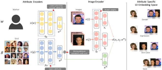
Figure 2.Context Embedding Networksare composed of three neural networks that are trained jointly. (Top-Left) A worker encoder network models workers’ annotation behavior and (Bottom-Left) a context encoder network models the attributes highlighted by a particular set of images. Jointly, these networks are referred to as the attribute encoders and are used to weight the embeddings produced by the image encoder network (Center). (Right) Our final embedding respects similarity estimates from each worker in the same low dimensional space where each dimension corresponds to a different visual attribute.

same number of annotations as 276 individual pairs. Across grids, real workers are often inconsistent with the attributes they use to cluster and the number of clusters they create. A pair of images(ig, jg)shown in the same grid,g,

clus-tered by workerwis assigned a positive labell = 1if they are grouped together andl= 0otherwise. This results in a training set of pairwise similarity labels

D={(w, g, ig, jg, l)|g= 1, ..., G}. (1)

3.1. Context Embedding Network (CEN)

Here we present out CEN model and define the loss func-tion used to train it. This involves joint training of three net-works which model workers, grid context, and image em-bedding respectively, see Fig.2. The first two networks are referred to asattribute encoderswhile the third is theimage encoder.

3.1.1 Worker Encoder

For the workers we define an attribute encoder networkqφ

which takes as input a one-hot encoding (o(·))of worker

w and outputs aK dimensional worker, attribute activa-tion, vectoraw = qφ(o(w)) = [aw1, ..., awK]. Eacha

w k, for

k = 1, ..., K, represents the degree of prior bias towards

attributekfor workerw. Once the network is trained, the output attribute activation vector models the worker’s prior preferences for each visual attribute. For example, a heav-ily biased worker that only attends to a single attributek∗

should have high activation for that particular attribute di-mensionaw

k∗. On the other hand, a worker that does not

have a strong preference for any particular attribute will

have weak attribute activations in allKdimensions and may be more influenced by the grid context.

3.1.2 Context Encoder

For an image grid containing S images, we define a con-text encoder networkpθ that takes as input aS-hot

encod-ing (s(·)) of the grid g and outputs aK dimensional grid

attribute activation vectorag = pθ(s(g)) = [ag₁, ..., ag_K].

Each ag_k for k = 1, ..., K represents the degree of

vi-sual prominence of attribute k for grid g. Once the net-work is trained, the grid attribute activation dimensions with high values should correspond to the most salient visual at-tributes highlighted by the input grid. Intuitively,attribute variancein the collection of images should influence which attributes are more noticeable to workers. For instance, a collection of images that is similar along all other attributes except onek∗should have a peak activation atag_k∗. On the

other hand, if the image set varies along many different at-tributes, ag _{should be close to uniformly distributed. The}

attribute vectorsaw_andag_{from the worker and context}

en-coders are combined to produce the final attribute encoder outputam_{(Fig.2Center).}

3.1.3 Image Encoder

We seek to learn a non-linear mapping from image ito a disentangled Euclidean coordinate xi where each

dimen-sion embeds the image into a one dimendimen-sional attribute specific subspace. To achieve this we use a Siamese Net-work architecture for the image encoder netNet-workfψ with

of imageiand outputs aKdimensional embedding vector

xi = fψ(o(i)) = [xi1, ..., xiK]. Although our image

em-bedding network learns an emem-bedding for each input image directly, with enough data it is possible to learn a feature extractor from the raw images [24]. Similarly, we present our model in terms of a pairwise loss, but it is also possi-ble to use a triplet loss for the image encoder. For brevity, from this point forward we omit the one and S-hot encoding function notationo(·), s(·).

3.2. Learning from the Crowd

By ignoring worker and context information, an embed-ding can be learned using Siamese networks [4], where the contrastive training lossLcis defined as

Lc(xi, xj) =ld(xi, xj) + (1−l) max{0, ξn−d(xi, xj)},

(2) whered(xi, xj) =kxi−xjk2is theL2distance between

imagei, j in embedding space. ξn is the negative margin

which prevents over-expanding the embedding manifold, andl ∈ {0,1}is the user provided label. This contrastive loss alone does not encourage the network to learn low di-mensional attribute specific embeddings as it assumes that all crowd workers compare images using the same visual attributes. To overcome this, we weight the L2 distance metric by the attribute activation vectors aw _andag_{. We}

hypothesize that a worker’s decision to cluster along a par-ticular attribute depends on both their prior preferences for specific visual attributes and the context highlighted by the set of images in the grid. Based on this assumption, we de-fine three variants of the distance metric weighted by the attribute activation vectors

d(xi, xj;aw) =kaw·(xi−xj)k2 =kqφ(w)·(fψ(i)−fψ(j))k2 (3) d(xi, xj;ag) =kag·(xi−xj)k2 =kpθ(g)·(fψ(i)−fψ(j))k2 (4) d(xi, xj;am) =kam·(xi−xj)k2 (5) =k(pθ(g) +qφ(w))·(fψ(i)−fψ(j))k2,

wheream=ag+awis the mixed attribute activation vector. After exploring different non-linear methods of mixing

agandam, we found that a simple summation sufficiently captures the relationship between the two biases. In the experiments section, we compare the performance of the above three different models. For the model in Eq. 5, bi-ased workers should have a concentrated worker attribute activation vectoraw_{which will dominate the mode of sum}

am_=aw_+ag_{. Alternatively, workers with weak prior}

pref-erences should have low worker attribute activationsaw_and

the grid attribute activationsagwill dictate the mode. Intu-itively, the attribute activation vector serves as a mask which indicates the embedding dimension that should be weighted heavily in the loss e.g. [24]. By encouraging sparsity inaw

andag _{along with ReLU non-linearities [16], we assume}

that grids that were clustered along one attribute will have a uni-modalam_{while grids that were clustered on a mixture}

of attributes will have a multi-modalam_{with peaks}

corre-sponding to the attribute dimensions used.

Inspired by the dual margin contrastive loss proposed in [28], we include a positive margin termξpin the loss

func-tion to prevent two images from overlapping in the embed-ding space which could lead to over fitting. This ensures that images will be pushed closer only if their current em-bedding is separated by more thanξp. We useato denote

the general attribute activation vector which can beag, aw, oram_{depending on the model variant}

Lc(xi, xj;a) =lmax{0, d(xi, xj;a)−ξp}+ (1−l) max{0, ξn−d(xi, xj;a)}.

(6)

A crowd worker’s decision to group two images is an ac-tive decision while choosing not to group images together can be seen as a more passive decision. This can become a problem when workers group images with different levels of detail. For example, a grid of shapes containing squares, tri-angles, circles, and stars might be clustered into two groups, squares and non-squares, by one worker. A second worker may group the images into the four different shape types. An embedding model might incorrectly assume that a dif-ferent attribute was used to separate the images, when it is in fact just a different level of granularity of ‘shape’ that is being used by both workers. To overcome this problem, we introduce an additional positive similarity weightγ, that captures the relative importance of the positive similarity labels compared to the dissimilarity labels

Lc(xi, xj;a) =γlmax{0, d(xi, xj;a)−ξp}+ (1−l) max{0, ξn−d(xi, xj;a)}.

(7)

This ensures that the model can learn the high level at-tributes when workers cluster with different levels of de-tail. In the example above, although cross category labels between circles, triangles, and stars are l = 0, the posi-tive labels generated within each circle, triangle, and star groups agree with the positive labels generated within the non-square group thus allowing the network to learn that the high level attribute, i.e. shape, used by both workers are the same. We show the impact ofγon the performance of our CEN in the supplementary materials.

3.3. Regularization

We add L1 penalties λ1kak1 to the attribute encoders

also regularize the embedding network with a L2 penalty

λ2kxk2to encourage regularity in the latent space. The final

loss function for our CENs is

LCEN(xi, xj;a) =γlmax{0, d(xi, xj;a)−ξp}+ (1−l) max{0, ξn−d(xi, xj)}+

λ1kak1+λ2kxik2+λ2kxjk2.

(8)

CENs require the number of dimensions K as a hyper-parameter. However, we observe that by settingKto a large number and byL1regularizingawandag, our model tends to only use a subset of the available embedding dimensions.

4. Experiments

Here we show that CENs can recover meaningful low-dimensional embeddings from noisy data. Network archi-tectures, training details, and hyperparameters tuning are described in the supplementary material. We perform ex-periments on the following three datasets:

CELEBAcontains images of different celebrity faces from which we select a random subset of 300 images [14]. For this dataset we instruct workers in advance to cluster on one attribute per grid respecting four visual attributes: gender, expression, skin color, and gaze direction. Although we ex-pect some workers to deviate from our instructions, having a definite ground truth set of attributes allow us to quantify the attribute retrieval accuracy. The CEN is unaware of the attribute selected for each grid. In total, 94 workers clus-tered 620 grids, yielding 170,000 similarity training pairs. RETINAis a medical dataset comprising of fundus images of the retina belonging to patients with varying degrees of diabetic retinopathy [8]. The images contain a number of visual indicators for the disease such as hard exudates (yel-low lesions dispersed throughout the retina). From 66 fun-dus images we crop out 300 image patches. These patches provide a localized view that may or may not contain indi-cator features of the disease. This dataset is more challeng-ing to discover meanchalleng-ingful attributes as the disease indicator features are visually subtle and the types of images are un-familiar to the crowd. We do not provide any instructions as to which attributes workers should attend to for this dataset. Here, 62 workers clustered 620 grids, yielding 170,000 sim-ilarity pairs.

BIRDSis a larger dataset composed of 1000 bird head im-ages made up of 16 randomly selected species from [26]. We use this dataset to demonstrate the scalability of our CENs. 252 workers clustered 3,000 grids yielding 820,000 similarity labels.

4.1. Data Collection

We use Amazon Mechanical Turk’s crowdsourcing plat-form to request crowd workers to cluster grids of images us-ing the GUI shown in Fig.3. Workers were presented with

Images are assigned colors to according to group membership Worker defines and describes each group

1 2

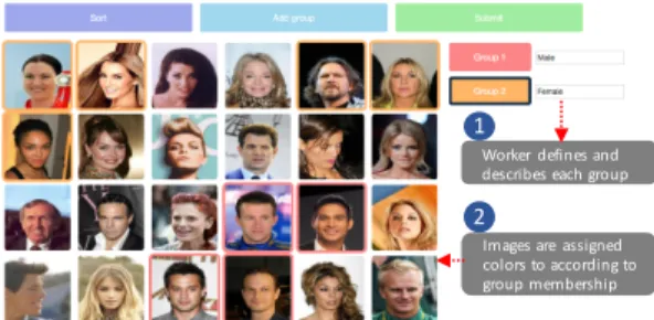
Figure 3.Data collection GUI.Workers group images they per-ceive to be visually similar by assigning them to different groups. They can create up to ten groups per grid of images.

a4×6 grid of images randomly sampled from the given dataset. Using up to ten possible groups, workers clustered images by first clicking on a group button on the right side of the page then clicking on the desired images. For each group they were asked to provide a short text description, used only for evaluation. The image, cluster, and worker ids were then converted into pairwise similarity labels (Eq.

1). Each worker clustered a minimum of ten grids in or-der to receive a reward, ensuring that the worker encoor-der network had sufficient data to learn from.

4.2. Baseline Comparisons

We compare results to four baseline methods and three variants of our model:

Standard Siamese Network e.g. [4]: Assumes that all pairwise similarity labels come from the same notion of similarity, as in Eq.2.

Standard Triplet Network e.g. [18]: Learns embeddings given similarity labels of the form ”A is more similar to B than C”.

Bayesian Crowd Clustering [6]: Workers are modeled as linear classifiers in the embedding space where both an en-tangledimage embedding and individual worker models are jointly learned with variational methods.

CSN [24]: Learns an entangled image embedding from similarity triplets which are disentangled by masks learned separately for each pre-known attribute. This baseline rep-resents the situation where the similarity dimension used by the worker isknown.

CEN-worker encoder only: This first variant of our model uses only worker modeling to learn attribute activations which weight the embeddings as in Eq.3.

CEN-context encoder only: Here we only model context information to weight the embeddings as in Eq.4.

CEN-mixture: Our full model, incorporates both worker and context information to learn a network that weights the worker biasaw_{and grid contexta}g_{as in Eq.5.}

4.3. Unsupervised Attribute Retrieval

First, we evaluate whether our CEN can accurately re-cover the four dominant attributes present in the CELEBA

dataset. For each grid g clustered by worker w, we take the mode dimension of the attribute activation vectorato be the model’s prediction, apred = argmaxkak. This is

the attribute that we predict was used to cluster the set of images. Again a can beaw_{, a}g _{or a}m _{depending on the}

model variant used. We then examine the annotations pro-vided by workers for each set of grids that map to a dif-ferentapred ∈ {1,2,3,4} and quantify the proportion of

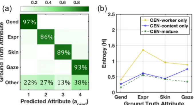
each attribute actually used. In Fig. 4(a) we show a confu-sion matrix illustrating that for each worker and grid pair, the CEN-mixture model is able to accurately predict which attribute was used. The row for gender and the first col-umn denote the proportion of grid submissions that have

apred = 1out of all the submissions that were clustered

along gender. For all attributes we obtain over85%attribute prediction accuracy. In Fig. 4(b) we plot the entropy H

of the distributionpfor each row of the confusion matrix whereHp = −Pplogp. High entropy indicates that the

ground truth attributes are scattered throughout the attribute predictions and vice versa. The CEN-mixture model outper-forms other variants across the four ground truth attributes. Although workers were encouraged to focus on four dif-ferent attribute options for this experiment, in practice they did not abide by our instructions and the proportion of noise in the raw data is significant. For the CELEBA dataset ap-proximately19.1%of the HITs completed were either clus-tered on different attributes such as “wearing sun glasses” (see Fig. 5) or noisy submissions where images were not separated into different groups. We also observed workers using different levels of detail when clustering on the same attribute. For example, for thegazeattribute some workers labeled “looking left”, “looking right”, etc. To demonstrate our model’s robustness, we perform all of our experiments on this raw data without filtering out annotation noise. For evaluation of the worker model learned by the worker en-coder, refer to the supplementary material.

4.4. Visualizing Disentangled Attributes

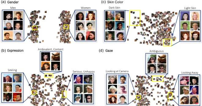
Fig.6shows the attribute specific embeddings of the four subspaces learned by the CEN for the CELEBA dataset. Fig.

6(a) shows that the embedding clearly separates the images according togender. On the very left of theexpression sub-space (Fig. 6(b)) we can see that people are smiling with teeth showing while on the right they show serious or un-happy expressions. In the middle we see ambiguous expres-sions. Fig. 6(c) shows the subspace embedded along the

skin colorattribute. On the two ends we see darker skinned and lighter skinned people. Fig. 6(d) shows the subspace forgaze directionof people, showing people that are either looking at the camera or away from it. Again, in the middle we see people wearing sunglasses or looking in ambiguous directions making it difficult to assess their gaze direction.

In Fig.7we show attribute specific embeddings learned

(a) 97% 89% 93% 86% 22% 27% 13% 38% (b)

Figure 4.Attribute retrieval accuracy.On the left we see the pre-dicted embedding dimensions from the CEN-mixture model com-pared to the ground truth visual attributes for the CELEBA dataset. On the right, we quantify how disentangled the learned embed-dings are. Lower entropy indicates models that better capture the ground truth attributes along individual embedding dimensions.

Gender Male, Female Men, Women Guys, Girls All men All females Expression Smiling, Not smiling Smiling, Frowning, Neutral Content, Undecided Thoughtful, Fearful Happy, Bored

Skin Color

Indian, African, Asian White, non-white Black, White Dark, Light, Tan White, Black Brown

Gaze

Looking, Not-looking Front, Left, Right Looking Straight, Crooked Side Pose, Front Pose Facing, Not-facing

Other Hat, No Hat Earing, No-Earing Hair up, Hair down Attractive, Ugly Humble, Arrogant I don’t know Celebrity Artist Musician Beard, no beard Wearing tie Black hair, Blond Sample Worker Annotations

Figure 5. Cluster Names. Keywords provided by workers for CELEBA. Colored labels indicate the manual grouping performed by us (only used for evaluation). Some workers use finer grained distinctions compared to others.

for the RETINAdataset in which no supervision was given to the workers for which attributes to pay attention to. Here we select four dimensions that are most highly activated from the learned ten dimensional embedding vector. Other attribute dimensions attain trivial activations. This shows that our CEN is robust to value ofK(please see supplemen-tary material for robustness analysis ofK). Fig.7(a) shows the first dimension seemingly showing the presence or ab-sence of the optic disc, a key feature of the retina. Fig.7(b) shows the subspace which discriminates between patches with blood vessels present and those without. Blood vessels are mostly concentrated and visually prominent around the optic disc, meaning that the two attributes are highly corre-lated. Regardless, our CEN is capable of distinguishing be-tween the two attributes, as we see that images displaying blood vessels without optic discs are correctly embedded in Fig. 7(a). Fig. 7(c) plots the attribute that groups laser scars (named after consulting with an ophthalmologist) and Fig.7(d) groups hard exudates, a key indicator for diagnos-ing diabetic retinopathy [10]. A comparison of embedding qualities between baselines are presented in the supplemen-tary material.

em-Figure 6.CELEBA - Attribute specific embeddings.Each plot shows one of the four different embedding dimensions produced by the CEN-mixture mode. The vertical axis in each subplot is randomly assigned for visualization purposes. We show representative images from the embeddings space in yellow boxes. We can see that the CEN learns to disentangle the attributes.

Figure 7.RETINA- Attribute specific embeddings.Here we show a subset of four of the ten embeddings dimensions produced by the CEN-mixture model for the RETINAdataset. Dimensions correlated well with visual features of diabetic retinopathy.

bedding space learned by the CEN for the BIRDSdataset. Each ellipse center corresponds to the mean of a Gaus-sian distribution fit to the embedding coordinates for each ground truth species. We observe 16 compact clusters that directly correlate to the 16 ground truth species. Please re-fer to the supplementary materials for confusion plots of the ground truth species vs embedding clusters.

4.5. Performance on Held-out Label Prediction

Here we quantify the generalization performance of the baseline methods on held-out pairwise label predictions

while varying the amount of training data. We measure the accuracy of the various model’s predictions on the sim-ilarity estimates for an unseen grid clustered by a known worker. For a grid inputg, worker inputw, and image pair

i, j, the model predicts i and j to be in the same group if d < (ξn +ξp)/2. The test set is made up of 15% of

the dataset and consists only of entire grids that were not present in the training set. This allows us to measure how well our CEN generalizes to new sets of images.

Fig. 9(a) shows results for the RETINA dataset. Stan-dard Siamese Networks and Triplet Networks fail to

cap-1 2 3 5 4

5

12

Figure 8. BIRDS- t-SNE embedding. Here we show a t-SNE [21] plot of the four dimensional embedding produced by the full CEN model for the BIRDSdataset. Indexed ellipses are centered at the Gaussian mean of different ground truth species. Clusters correlated well with ground truth species of birds.

CEN–mix outperforms (a) (b) Pre-known Similarity Attribute Pre-known Similarity Attribute CEN–mix outperforms

Figure 9.Held-out label prediction.Prediction accuracy on held out labels for the RETINAand BIRDSdatasets plotted against the amount of available data during training.

ture the multiple attributes used to cluster the images and have the lowest prediction accuracy of58.1%and58.5%. The Bayesian Crowd Clustering model, CEN worker, and CEN grid only models attain similar prediction accuracies of 67%. For the more challenging RETINA dataset work-ers found it difficult to discover various attributes to cluster on and thus often fixated on a single attribute on all their HITs. However, we still benefit from modeling the context as the CEN-mixture model achieves prediction accuracy of

69.4%. The CSN model with learned masks obtains the highest accuracy of75.5%, but it is important to note that this model was trained on triplets pre-labeled with the true similarity attributes used to cluster them.

Fig. 9(b) shows the pairwise prediction accuracy for each model plotted against a varying number of training samples for the BIRDSdataset. The Bayesian Crowd Clus-tering model, CEN worker, and CEN grid only models attain similar prediction accuracies of 62%. The CEN-mixture substantially outperforms all baselines with a pre-diction accuracy of 70.5%which is only 3.5% below the accuracy of the CSN model which uses ground truth labels.

4.6. Image Grid Synthesis

Being able to synthesize image grids that highlight spe-cific attributes may useful in active learning where the data collector seeks to obtain similarity estimates along particu-lar visual attributes. We randomly generate ten million im-age grids and individually pass them through the context encoder and extract the grid attribute activation vectorsag

for each grid. We take a softmax activation over the ag_s

and select grids that have low entropy, thus choosing grids that are highly expressive of a particular attribute. Fig. 10

shows one generated grid with the lowest entropy for the gaze attribute. We see low variance among the images along other attributes such as gender, skin color, and gaze direc-tion while there is high variance for the gaze attribute. This suggests that in order for an image grid to emphasize a par-ticular attribute, the contained items should be similar in all but one high variance attribute.

High variance along “Gaze”

Figure 10. Synthesized image grids. Our context encoder can be used to generate collections of images that highlight specific attributes. The shown grid has high variance along the gaze direc-tion attribute and low variance for the others.

5. Conclusion and Future Work

We proposed a novel deep neural network that jointly learns attribute specific embeddings, worker models, and grid context models from the crowd. By comparing to sev-eral baseline methods, we show that our model more accu-rately predicts the attributes used by individual workers and as a result produces better quality image embeddings.

In future work we plan to incorporate relative similarity estimates and the learning of representations directly from images [24,18]. Although currently we model each worker individually, in practice there may be similarity between different workers that could be discovered through cluster-ing [9]. Finally, our grid context encoder enables us to gen-erate sets of images that highlight specific attributes. By combining this encoder with active learning we can poten-tially speed up the collection of annotations from the crowd [19,13].

References

[1] E. Amid and A. Ukkonen. Multiview triplet embed-ding: Learning attributes in multiple maps. InICML, 2015.2

[2] T. L. Berg, A. C. Berg, and J. Shih. Automatic at-tribute discovery and characterization from noisy web data. InECCV, 2010.2

[3] S. Branson, G. Van Horn, and P. Perona. Lean crowd-sourcing: Combining humans and machines in an on-line system. InCVPR, 2017.2

[4] J. Bromley, J. W. Bentz, L. Bottou, I. Guyon, Y. Le-Cun, C. Moore, E. S¨ackinger, and R. Shah. Signature verification using a ”siamese” time delay neural net-work.IJPRAI, 1993. 2,4,5

[5] A. Farhadi, I. Endres, D. Hoiem, and D. Forsyth. De-scribing objects by their attributes. InCVPR, 2009.

2

[6] R. G. Gomes, P. Welinder, A. Krause, and P. Perona. Crowdclustering. InNIPS, 2011.2,5

[7] G. Jurman and C. Furlanello. A unifying view for performance measures in multi-class prediction.

arXiv:1008.2908, 2010. 12

[8] Kaggle. Kaggle Diabetic Retinopathy Detec-tion. https://www.kaggle.com/c/diabetic-retinopathy-detection, 2015. 5

[9] H. Kajino, Y. Tsuboi, and H. Kashima. Clustering crowds. InAAAI, 2013.8

[10] R. V. J. P. H. K¨alvi¨ainen and H. Uusitalo. Diaretdb1 diabetic retinopathy database and evaluation protocol. InMIUA, 2007. 6

[11] A. Kovashka, O. Russakovsky, L. Fei-Fei, K. Grau-man, et al. Crowdsourcing in computer vision. Foun-dations and Trends in Computer Graphics and Vision, 2016.2

[12] C. H. Lampert, H. Nickisch, and S. Harmeling. Learn-ing to detect unseen object classes by between-class attribute transfer. InCVPR, 2009. 2

[13] L. Liang and K. Grauman. Beyond comparing image pairs: Setwise active learning for relative attributes. In

CVPR, 2014.9

[14] Z. Liu, P. Luo, X. Wang, and X. Tang. Deep learning face attributes in the wild. InICCV, 2015. 5

[15] S. Maji and G. Shakhnarovich. Part and attribute dis-covery from relative annotations.IJCV, 2014.2

[16] V. Nair and G. E. Hinton. Rectified linear units im-prove restricted boltzmann machines. InICML, 2010.

4

[17] D. Parikh and K. Grauman. Relative attributes. In

ICCV, 2011.2

[18] F. Schroff, D. Kalenichenko, and J. Philbin. Facenet: A unified embedding for face recognition and cluster-ing. InCVPR, 2015. 2,5,8

[19] O. Tamuz, C. Liu, S. Belongie, O. Shamir, and A. T. Kalai. Adaptively learning the crowd kernel. ICML, 2011.2,9

[20] T. Tian, N. Chen, and J. Zhu. Learning attributes from the crowdsourced relative labels. InAAAI, 2017. 1,2

[21] L. van der Maaten and G. Hinton. Visualizing data using t-sne.JMLR, 2008. 2,8,11

[22] L. van der Maaten and K. Weinberger. Stochastic triplet embedding. In Machine Learning for Signal Processing, 2012. 1,2

[23] G. Van Horn, S. Branson, R. Farrell, S. Haber, J. Barry, P. Ipeirotis, P. Perona, and S. Belongie. Building a bird recognition app and large scale dataset with cit-izen scientists: The fine print in fine-grained dataset collection. InCVPR, 2015. 1

[24] A. Veit, S. Belongie, and T. Karaletsos. Conditional similarity networks. InCVPR, 2017.1,2,4,5,8

[25] R. K. Vinayak and B. Hassibi. Crowdsourced clus-tering: Querying edges vs triangles. InNIPS, 2016.

2

[26] C. Wah, S. Branson, P. Welinder, P. Perona, and S. Be-longie. The Caltech-UCSD birds-200-2011 dataset. 2011.5

[27] C. Wah, G. Van Horn, S. Branson, S. Maji, P. Perona, and S. Belongie. Similarity comparisons for interac-tive fine-grained categorization. InCVPR, 2014. 2

[28] X. Wang, K. M. Kitani, and M. Hebert. Contextual visual similarity. arXiv:1612.02534, 2016.2,4

[29] P. Welinder, S. Branson, S. J. Belongie, and P. Perona. The multidimensional wisdom of crowds. InNIPS, 2010.2

[30] J. Whitehill, T.-f. Wu, J. Bergsma, J. R. Movellan, and P. L. Ruvolo. Whose vote should count more: Op-timal integration of labels from labelers of unknown expertise. InNIPS, 2009. 2

[31] M. Wilber, I. S. Kwak, and S. Belongie. Cost-effective hits for relative similarity comparisons. InHCOMP, 2014.2

[32] M. Wilber, I. S. Kwak, D. Kriegman, and S. Belongie. Learning concept embeddings with combined human-machine expertise. InICCV, 2015. 2

[33] Z. Zhu, C. Yin, B. Qian, Y. Cheng, J. Wei, and F. Wang. Measuring patient similarities via a deep ar-chitecture with medical concept embedding. InICDM, 2016.2

Supplementary Results

Here we provide the model architecture and training de-tails for our CEN models along with additional experimen-tal results.

A. Model Parameters

For both datasets, the worker and context encoders are fully connected neural networks consisting of two hidden layers each with200neurons with ReLU activations. The image encoder has one hidden layer with200units and out-puts aKdimensional embedding vector. For the CELEBA dataset, the embedding dimensionKis set to four since we provide the workers with four different attributes to cluster on. For the RETINA dataset, we setK = 10since we do not knowa priorihow many different attributes the workers will use. We jointly train the three encoders with a mini-batch size of100using ADAM withα= 0.001, β1 = 0.9,

andβ2 = 0.999. We experimented with various learning

ratesα∈ {0.00001,0.0001,0.001,0.01}and found that the CEN performance was robust to these variations. The regu-larization constants are set toλ1= 5E−6andλ2= 0.001.

We experimented withλ1∈ {1E−6,5E−6,1E−5,5E− 5}, λ2 ∈ {0.0001,0.0005,0.001,0.005,0.01}and saw that

the prediction accuracy decreases whenλ1>5E−6, λ2> 0.001, but relatively stable otherwise. Hence, we choose the largest possible learning rate to reduce training time. Table S1.Impact of positive similarity weightγon label predic-tion accuracy.γ= 6was used for all results presented in the main paper.

γ= 1 γ= 4 γ= 6 γ= 8 γ= 10 CELEBA 68.5% 69.8% 69.8% 69.3% 69.2%

RETINA 68.1% 69.3% 69.4% 69.1% 68.7%

The positive margin, negative margin, and positive sim-ilarity weight are each set to ξp = 1, ξn = 6 and γ = 5, respectively. The prediction accuracy decreased when

ξn/ξp<4. We experimented with varying positive

similar-ity weightsγ ∈ {1,2, ...,10}and found thatγ ={4,5,6}

achieves similar best prediction accuracy when trained on the full dataset. In TableS1we show the impact ofγ on the label prediction accuracy for both datasets. The opti-mum value ofγ should be expected to change depending on the variance in the level of detail workers cluster grids. Models were trained for 20 epochs which we determined to be sufficient for learning interpretable embeddings. When utilizing all the data from 620 HITs, the training time was on average 2.5 minutes for both datasets running on CPUs (Macbook Pro 13-inch, Late 2012, 2.5 GHz Intel Core i5, 8GB RAM, Apple, CA, USA). Upon publication we will make the code for our GUI and CEN model available.

(a) (b)

(c)

(d)

(e) Intensity

Figure S1.Visualizing the worker model. On the left we see the predicted attribute activation vectors for each worker from the CELEBA dataset. Attribute dimension labels were inferred from worker annotations. Brighter colors indicate a stronger preference for a given attribute. On the right we show the actual attributes used by a set of representative workers inferred from their text annotations. We can see that our worker attribute predictions are consistent with the actual attributes used by the workers.

B. Interpretation of the Worker Model

We explore the learned attribute activation vectorsaw_for

each worker to examine if their prior biases were captured by the worker encoder. The output attribute activation vec-tors for each of the 94 workers are shown in Fig. S1(a) as a stacked heatmap. On the right side of Fig. S1, we show the distribution of attributes that four representative workers have used over the course of performing ten HITs, inferred from their text annotations. Fig.S1(a) shows that our model predicts a high activation inaw3 for worker 24. In Fig.S1(b)

we can see that this worker consistently used the skin color attribute for all ten HITs they performed. This indicates that worker 24 had a strong prior bias towards grouping based on skin color and was unaffected by the different contexts formed by the grid. Note that it is highly unlikely that all ten randomly generated grids shown to worker 24 highlighted the skin color attribute. Fig.S1(c) shows that worker 35 re-lied mainly on the expression attribute. Similarly for worker 45 we observe a strong bias towards the gender attribute as the worker encoder outputs a high activation foraw

1. Worker

88 used a variety of attributes suggesting that they are more sensitive to the context provided by the grid. We observe a near uniform attribution activation vector for this worker.

C. Comparison of the Joint Embeddings

We compare the quality of the embeddings for the CELEBA dataset produced by the CEN-mixture model with those learned by baseline approaches that do not model con-text. We project the four dimensional joint embedding

vec-Bayesian Crowd Clustering

Gender Expression Skin Color Gaze

CEN -Worker Only CEN -Mixed Model

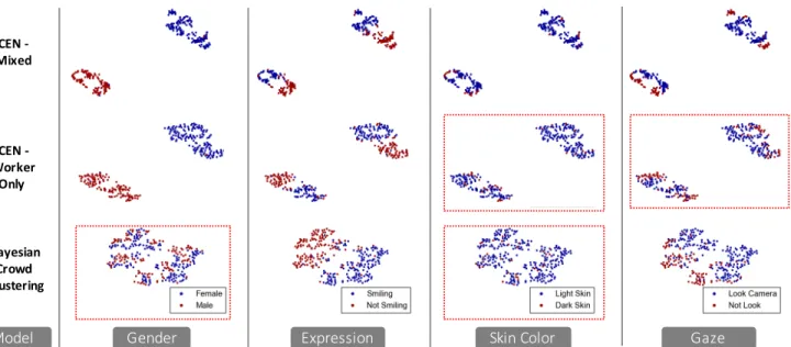
Figure S2.Comparing embedding quality. 2D t-SNE projections of the four dimensional joint embedding space for three embedding models on the CELEBA dataset. Colors denote binarized ground truth categories for each of the four attributes: gender, expression, skin color, and gaze direction. Dotted red boxes highlight attributes for which the CEN-mixture model produces more compact embeddings compared to the baselines.

Pre-known Similarity Attribute

CEN–mix outperforms

Figure S3.Held-out Label Prediction on CELEBA. Prediction accuracy on held out labels for the CELEBA dataset plotted against the amount of available data during training.

torsxidown to two dimensions using t-SNE [21] and color

code each point according to its ground truth attribute. For each attribute, the ground truth categories were binarized for simplicity, i.e. smiling vs not smiling. In Fig. S2we show the low dimensional embeddings learned by the CEN-mixture model, CEN-worker only model, and the Bayesian Crowd Clustering baseline. The CEN-mixture model bet-ter separates the ground truth categories in the embedding space. This shows the positive impact of modeling context. The worker encoder only model finds well separated em-beddings along the gender and expression attribute (which are relatively easy to distinguish) but does not perform well on the skin color and gaze attributes (which are attributes that workers more often disagree on). The Bayesian Crowd

Hard Exu. Opt. Disc

Veins _{Las. Cuts}

Hard Exu. Opt. Disc

Veins Las. Cuts

Hard Exu.

Opt. Disc Veins _{Las. Cuts}

Figure S4.Varying the embedding dimension for the RETINA

dataset. We plot the average activations for each dimension ofam produced by the CEN-mixture model for three different values of embedding dimensionK. Red labels were inferred from the text annotations.

Clustering baseline has difficulty separating the gender and skin color attributes.

D. Heldout Label Predictions on

Fig. S3(a) shows the pairwise prediction accuracy for each model plotted against a varying number of training samples for the CELEBA dataset. Standard Siamese Net-works and Triplet NetNet-works fail to capture the multiple at-tributes used to cluster the images and have the lowest pre-diction accuracy of58.1%and58.5%. The Bayesian Crowd Clustering method slightly improves on that with an accu-racy59.1%. The worker only variant of our model achieves a prediction accuracy of62.1%. This is superior to Siamese Networks and Bayesian Crowd Clustering but still fails to

capture the tendency of workers to shift their clustering cri-terion based on the context highlighted by images in the grid. The context only model variant performs substan-tially better with a prediction accuracy of65.2%. This indi-cates that the context information is indeed influencing the worker’s decisions. Finally, the CEN-mixture outperforms all previous baselines with a prediction accuracy of69.8%. The CSN model with learned masks obtains the highest ac-curacy of77.3%, but it is important to note that this model was trained on triplets pre-labeled with the true similarity attributes used to cluster them. The CEN-mixture model achieves strong predictive performance without any prior knowledge of the similarity attributes.

E. Prior Number of Attributes

For theRETINAdataset, we do not know the number of number of attributes the workers will use. Hence, we set

K = 10which serves as our prior guess of an upperbound on the number of attributes the workers are going to use. Although the attribute vector dimension was set toK= 10, we observed that four dimensions were consistently highly activated across different values ofK. In Fig. S4we see that the attribute dimensions we selected are the four most highly activated dimensions ofamforK= 10,20,and30.

Figure S5.Confusion plot for the BIRDSdataset.

F. Clustering Learned Embeddings

For the BIRDS dataset, we perform K-means cluster-ing on the learned 4 dimensional embeddcluster-ing space with

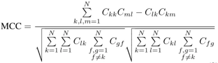
K = 16 and compare the ground truth bird species of an image with its assigned cluster. To quantify the agreement between the ground truth species and the learned clusters, we use the multi-class version of Matthew’s Correlation Co-efficient (MCC) [7], where MCC= 1indicates perfect pre-diction, and a value between −1 and0 denotes total dis-agreement depending on the true distribution.

MCC= N P k,l,m=1 CkkCml−ClkCkm v u u t N P k=1 N P l=1 Clk N P f,g=1 f6=k Cgf v u u t N P k=1 N P l=1 Ckl N P f,g=1 f6=k Cf g (9) The confusion plot in Fig. S5reveals high correlation (MCC = 0.914) between the ground truth species and the learned clusters, suggesting that the CEN is able to make fine-grained distinctions amongst bird species despite highly noisy training data (25.6%for the BIRDSdataset).

G. Limitations

Our context model assumes that the ordering of the im-ages in the grid does not effect clustering behavior. In prac-tice this may have some effect on the workers. To produce disentangled attribute vectors we assume that a majority of the grids are clustered along a single attribute. However, from our experiments we observe that this only has to be very weakly satisfied as many workers used a mixture of attributes.