Stephen Drape
St John’s CollegeThesis submitted for the degree of Doctor of Philosophy
at the University of Oxford
Stephen Drape St John’s College University of Oxford
Thesis submitted for the degree of Doctor of Philosophy Trinity Term 2004
Abstract
Anobfuscationis a behaviour-preserving program transformation whose aim is to make a program “harder to understand”. Obfuscations are applied to make reverse engineering of a program more difficult. Two concerns about an obfuscation are whether it preserves behaviour (i.e.it iscorrect) and the degree to which it maintains efficiency. Obfuscations are applied mainly to object-oriented programs but constructing proofs of correctness for such obfuscations is a challenging task. It is desirable to have a workable definition of obfuscation which is more rigorous than the metric-based definition of Collberg et al. and overcomes the impossibility result of Baraket al. for their strong cryptographic definition.
We present a fresh approach to obfuscation by obfuscating abstract data-typesallowing us to develop structure-dependent obfuscations that would other-wise (traditionally) not be available. We regard obfuscation as data refinement enabling us to produce equations for proving correctness and we model the data-type operations as functional programs making our proofs easy to construct. For case studies, we examine different data-types exploring different areas of computer science. We consider lists letting us to capture array-based obfusca-tions,setsreflecting specification based software engineering,trees demonstrat-ing standard programmdemonstrat-ing techniques and as an example of numerical methods we considermatrices.
Our approach has the following benefits: obfuscations can be proved correct; obfuscations for some operations can bederived and random obfuscations can be produced (so that different program executions give rise to different obfusca-tions). Accompanying the approach is a new definition of obfuscation based on measuring the effectiveness of an obfuscation. Furthermore in our case studies the computational complexity of each obfuscated operations is comparable with the complexity of the unobfuscated version. Also, we give an example of how our approach can be applied to implement imperative obfuscations.
I
The Current View of Obfuscation
11
1 Obfuscation 12 1.1 Protection . . . 12 1.2 Obfuscation . . . 13 1.3 Examples of obfuscations . . . 14 1.3.1 Commercial Obfuscators. . . 15 1.3.2 Opaque predicates . . . 16 1.3.3 Variable transformations. . . 16 1.3.4 Loops . . . 17 1.3.5 Array transformations . . . 18 1.3.6 Array Splitting . . . 18 1.3.7 Program transformation . . . 19 1.3.8 Array Merging . . . 20 1.3.9 Other obfuscations . . . 20 1.4 Conclusions . . . 212 Obfuscations for Intermediate Language 22 2.1 .NET . . . 22
2.1.1 IL Instructions . . . 22
2.2 IL obfuscations . . . 25
2.2.1 Variable Transformation . . . 25
2.2.2 Jumping into while loops . . . 26
2.3 Transformation Toolkit . . . 27
2.3.1 Path Logic Programming . . . 28
2.3.2 Expression IL . . . 29
2.3.3 Predicates for EIL . . . 31
2.3.4 Modifying the graph . . . 32
2.3.5 Applying transformations . . . 33
2.3.6 Variable Transformation . . . 33
2.3.7 Array Splitting . . . 34
2.3.8 Creating an irreducible flow graph . . . 37
2.4 Related Work . . . 40 2.4.1 Forms of IL . . . 40 2.4.2 Transformation Systems . . . 41 2.4.3 Correctness . . . 41 2.5 Conclusions . . . 42 2
3 Techniques for Obfuscation 44
3.1 Data-types . . . 44
3.1.1 Notation. . . 45
3.1.2 Modelling in Haskell . . . 46
3.2 Obfuscation as data refinement . . . 48
3.2.1 Homogeneous operations. . . 49
3.2.2 Non-homogeneous operations . . . 50
3.2.3 Operations using tuples . . . 51
3.2.4 Refinement Notation . . . 51
3.3 What does it mean to be obfuscated? . . . 52
3.4 Proof Trees . . . 54
3.4.1 Measuring. . . 56
3.4.2 Comparing proofs . . . 56
3.4.3 Changing the measurements. . . 59
3.4.4 Comments on the definition . . . 60
3.5 Folds . . . 60
3.6 Example Data-Types. . . 61
III
Data-Type Case Studies
62
4 Splitting Headaches 63 4.1 Generalising Splitting . . . 634.1.1 Indexed Data-Types . . . 63
4.1.2 Defining a split . . . 64
4.1.3 Example Splits . . . 65
4.1.4 Splits and Operations . . . 66
4.2 Arrays . . . 68 4.2.1 Array-Split properties . . . 69 4.3 Lists . . . 71 4.3.1 List Splitting . . . 72 4.3.2 Alternating Split . . . 73 4.3.3 Block Split . . . 77
4.4 Random List Splitting . . . 82
4.4.1 Augmented Block Split . . . 87
4.4.2 Padded Block Split. . . 89
4.5 Conclusions . . . 90
5 Sets and the Splitting 92 5.1 A Data-Type for Sets . . . 92
5.2 Unordered Lists with duplicates. . . 92
5.2.1 Alternating Split . . . 94
5.3 Strictly Ordered Lists . . . 95
5.3.1 Alternating Split . . . 96
5.3.2 Block Split . . . 98
5.4 Comparing different definitions . . . 99
5.4.1 First Definition . . . 100
5.4.2 Second Definition. . . 101
5.5 Conclusions . . . 106
6 The Matrix Obfuscated 107 6.1 Example . . . 107
6.2 Matrix data-type . . . 108
6.2.1 Definitions of the operations . . . 109
6.3 Splitting Matrices . . . 110
6.3.1 Splitting in squares. . . 110
6.3.2 Modelling the split in Haskell . . . 112
6.3.3 Properties . . . 113
6.3.4 Deriving transposition . . . 113
6.3.5 Problems with arrays . . . 115
6.4 Other splits and operations . . . 116
6.4.1 Other Splits. . . 116
6.4.2 A more general square splitting . . . 117
6.4.3 Extending the data-type of matrices . . . 118
6.5 Conclusions . . . 118
7 Cultivating Tree Obfuscations 119 7.1 Binary Trees . . . 119
7.1.1 Binary Search Trees . . . 120
7.2 Obfuscating Trees . . . 123
7.2.1 Ternary Trees. . . 123
7.2.2 Particular Representation . . . 124
7.2.3 Ternary Operations . . . 126
7.2.4 Making Ternary Trees . . . 127
7.2.5 Operations for Binary Search Trees. . . 128
7.2.6 Deletion . . . 128 7.3 Other Methods . . . 129 7.3.1 Abstraction Functions . . . 130 7.3.2 Heuristics . . . 131 7.4 Conclusions . . . 132
IV
Conclusions
133
8 Conclusions and Further Work 134 8.1 Discussion of our approach to Obfuscation . . . 1348.1.1 Meeting the Objectives . . . 134
8.1.2 Complexity . . . 135 8.1.3 Definition . . . 136 8.1.4 Randomness . . . 136 8.1.5 Contributions . . . 137 8.2 Further Work . . . 137 8.2.1 Deobfuscation. . . 138 8.2.2 Other techniques . . . 138 4
A List assertion 144
A.1 Unobfuscated version. . . 144
A.2 Alternating Split for Lists . . . 145
A.2.1 Version 1 . . . 145
A.2.2 Version 2 . . . 147
A.3 Block Split for Lists . . . 149
A.4 Augmented Split . . . 152
A.5 Augmented Block Split. . . 154
A.6 Padded Block Split . . . 156
A.7 Comparing the proofs . . . 158
B Set operations 159 B.1 Span Properties. . . 159
B.2 Insertion for the alternating split . . . 164
C Matrices 166 C.1 Rewriting the definition . . . 166
C.2 Using fold fusion . . . 167
D Proving a tree assertion 169 D.1 Producing a binary tree from a list . . . 169
D.1.1 Operations . . . 169
D.1.2 Proving Properties . . . 170
D.1.3 Proving the assertion. . . 172
D.2 Producing a binary tree from a split list . . . 174
D.2.1 Operations . . . 174
D.2.2 Preliminaries . . . 174
D.2.3 Proof of the assertion . . . 179
D.3 Producing a ternary tree from a list . . . 180
D.3.1 Operations . . . 180
D.3.2 Proof . . . 180
D.4 Producing a ternary tree from a split list. . . 182
D.4.1 Proof . . . 182
D.5 Comparing the proofs . . . 184
E Obfuscation Example 185
1 An example of obfuscation. . . 8
1.1 Fibonacci program after an array split . . . 20
2.1 Some common IL instructions . . . 23
2.2 IL for a GCD method . . . 24
2.3 Output from Salamander . . . 27
2.4 Syntax for a simple subset of EIL . . . 30
2.5 Some common predicates . . . 32
2.6 Predicates for replacing assignments . . . 35
2.7 Definition ofreplace array for assignments. . . 36
2.8 Flow graph to build a conditional expression . . . 37
2.9 Flow graph to create jump into a loop . . . 38
2.10 Code for theirred jump method . . . 39
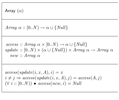
3.1 Data-type for Arrays . . . 47
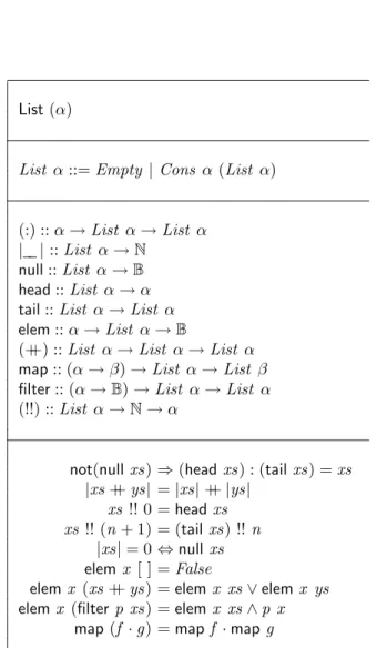
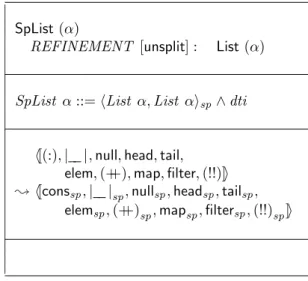
4.1 Data-type for Lists . . . 70
4.2 Data-type for Split Lists . . . 72
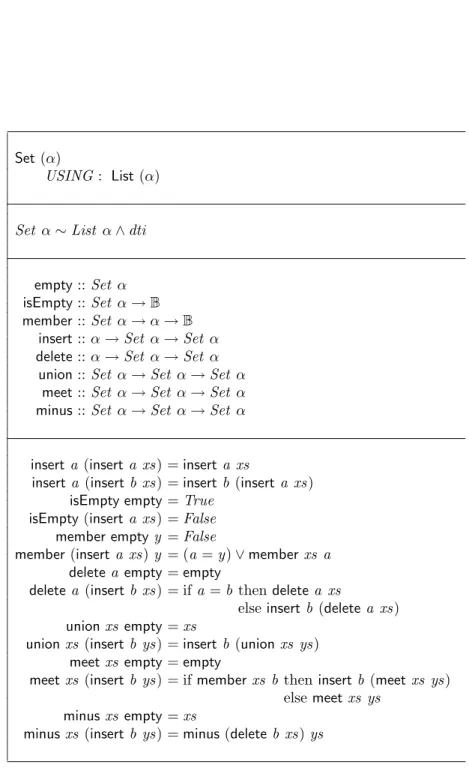
5.1 Data-type for Sets . . . 93
6.1 Data-type for Matrices . . . 109
7.1 Data-Type for Binary Trees . . . 120
7.2 Data-Type for Binary Search Trees . . . 121
7.3 Data-Type for Ternary Trees . . . 124
E.1 Original Program. . . 186
Homer: “All right brain, you don’t like me and I don’t like you. But let’s just do this and I can get back to killing you with beer.”
The Simpsons —The Front (1993)
In this thesis, we consider theobfuscation of programs. “To Obfuscate” means “To cast into darkness or shadow; to cloud, obscure”. From a Computer Science perspective, an obfuscation is a behaviour-preserving program transfor-mation whose aim is to make a program “harder to understand”. Obfuscations are applied to a program to make reverse engineering of the program more dif-ficult. Two concerns about an obfuscation are whether it preserves behaviour (i.e. it iscorrect) and the degree to which it maintains efficiency.
Example
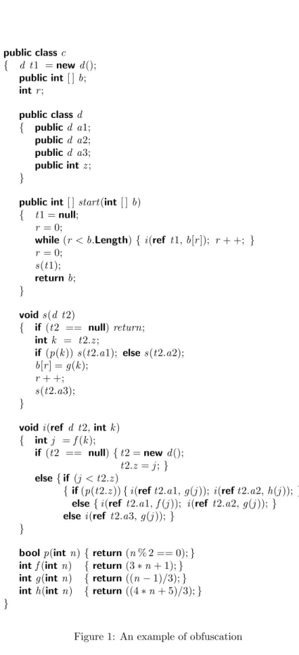
As an example of obfuscation, consider the program in Figure1. The method
start takes an integer value array as input and the array is returned from the method. But what does this method do to the elements of the array? The obfuscation was achieved by using some of the methods outlined in this thesis.
Aims of the thesis
The current view of obfuscation (in particular, the paper by Collberget al.[10]) concentrates on object-oriented programs. In [10], obfuscations for constructs such as loops, arrays and methods are stated informally: without proofs of correctness. Constructing proofs of correctness for imperative obfuscations is a challenging task.
We offer an alternative approach based on data refinement and functional programming. We want our approach to have the following objectives:
• to yield proofs of correctness (or even yield derivations) of all our obfus-cations
• to use simple, established refinement techniques, leaving the ingenuity for obfuscation
• to generalise obfuscations to make obfuscations more applicable.
public classc { d t1 =newd(); public int[ ]b; intr; public classd { publicd a1; publicd a2; publicd a3; public int z; }
public int[ ]start(int [ ]b) { t1 =null;
r = 0;
while(r <b.Length){i(ref t1,b[r]); r+ +; }
r = 0; s(t1); returnb; } voids(d t2) { if (t2 == null)return; int k = t2.z; if (p(k))s(t2.a1); elses(t2.a2); b[r] =g(k); r + +; s(t2.a3); }
voidi(ref d t2,int k) { int j =f(k);
if (t2 == null){t2 =new d();
t2.z =j; } else {if (j <t2.z)
{if(p(t2.z)){i(reft2.a1,g(j));i(reft2.a2,h(j));} else {i(ref t2.a1,f(j)); i(ref t2.a2,g(j));} elsei(ref t2.a3,g(j));}
}
boolp(intn){ return(n% 2 == 0);} intf(intn) { return(3∗n+ 1);} intg(intn) { return((n−1)/3);} inth(intn) { return((4∗n+ 5)/3);} }
We study abstract data-types (consisting of a local state accessible only by declared operations) and define obfuscations for the whole data-type. In other words, we obfuscate the state of the data-type under the assumption that the only way it is being accessed is via the operations of the type. Different operations (on a given state) may require different obfuscations.
To date, obfuscation has been an area largely untouched by the formal method approach to program correctness. We regard obfuscation as data re-finement allowing us to produce equations for proving correctness. We model the data-type operations as functional programs. That enables us to establish correctness easily as well as providing us with an elegant style in which to write definitions of our operations. Two benefits of using abstract data-types are that we can specify obfuscations which exploit structural properties inherent in the data-type; and the ability to create random obfuscations. We also provide a new definition of obfuscation that avoids the impossibility problem considered by Baraket al.[6] and is appropriate for our data-type approach.
Structure of the thesis
The thesis is structured as follows:• In Chapters 1 and 2 we consider the current view of obfuscation. In Chapter1we discuss the need for obfuscation and summarise some of the obfuscations from [10]. Also we evaluate the definitions for obfuscation given in [6,10]. In Chapter2we look at the .NET Intermediate Language [23] and discuss joint work with Oege de Moor and Ganesh Sittampalam that allows us to write some specifications of obfuscations for Intermediate Language.
• In Chapter3we give an alternative view of obfuscation by concentrating on abstract data-types. We use data refinement and functional program-ming to produce a framework that allows us to prove the correctness of obfuscations (or even to derive them) and we give a definition of obfusca-tion pertinent to our approach.
• In Chapter4we use our approach to generalise an obfuscation calledarray splitting and we show how to split more general data-types.
• The next three chapters concentrate on specific case studies for different data-types. In Chapters5 and6we use the results on data-type splitting to show how to construct obfuscations for sets and matrices. In Chapter
7we give a transformation suitable for obfuscating binary trees.
• Finally, in Chapter8, we summarise our results and discuss possible areas for future work.
Contributions
The thesis provides the following contributions.
Using established work on refinement, abstract data-types and functional programming, a new approach to obfuscation is developed. This approach has the following benefits:
• Obfuscations can be proved correct.
• The obfuscations of some operations can be derivedfrom their unobfus-cated versions.
• Random obfuscations can be produced so that different program execu-tions give rise to different obfuscaexecu-tions, making them particularly obscure. The approach is accompanied by a new definition, based on measuring the effectiveness of an obfuscation. Furthermore, in the case studies included here, our obfuscations are (close to) optimal in the sense that the computational complexity of each obfuscated operation is comparable with the complexity of the unobfuscated version.
Notation
We will use various programming languages in this thesis and so we adopt the following conventions to differentiate between the different languages:
• C#: We usebold sans seriffor standard keywords anditalicsfor variables. • IL: We usetypewriterfont for the whole language.
• Prolog: We write all predicates initalics.
• Haskell: Operations are written insans serif font, variables initalics and keywords in normal font.
Type declarations are of the formf ::T — we use this notation instead of the more usual notation f : T so that type statements and list constructions are not confused.
We denote lists (and occasionally arrays) by [ ], sets by { }, sequences byh[ ]iand a split data-type by h i(see Chapter 4for the definition of split data-types). We assume the following types: N(natural numbers),Z(integers) and B (Booleans). Also, we write [a..b] to denote {i :: Z |a ≤ i ≤ b} and similarly [a..b) to denote{i::Z|a≤i<b}.
Acknowledgements
Thanks to Jeff Sanders for his continual support and encouragement during his time as my supervisor. This thesis would have been impossible to complete without Jeff’s constant help and advice.
Various members of the Programming Research Group have given their time to provide comments and advice, in particular: Richard Brent, Rani Ettinger, Yorck H¨unke, Damien Sereni, Barney Stratford and Irina Voiculescu.
Thanks also to Geraint Jones and Simon Thompson for providing useful feedback during the viva.
The Current View of
Obfuscation
Obfuscation
Scully: “Not everything is a labyrinth of dark conspiracy. And not everyone is plotting to deceive, inveigle and obfuscate”
The X-Files — Teliko(1996)
This chapter introduces the notion of obfuscation, summarises specific ex-amples given in the original paper [10] and discusses some related work.
1.1
Protection
Suppose that a programmer develops a new piece of software which contains a unique innovative algorithm. If the programmer wants to sell this software, it is usually in the programmer’s interest that the algorithm should remain secret from purchasers. What can the programmer do to stop the algorithm from being seen or modified by a client? A similar issue arises when a piece of software contains a date stamp that allows it to be used for a certain length of time. How can we stop people from identifying (and changing) the date stamp? We will assume that it is possible for an executable file to be decompiled to a high-level language and so the source code of an executable can be studied. In fact, this is the situation with Java Bytecode and the .NET framework (see Chapter2 for more details). Therefore, we need to consider ways of protecting software so that it is hard to understand a program after decompilation. Here are some of the protections that are identified in [10]:
• Server-side execution— this involves clients remotely accessing the soft-ware from a programmer’s site. The downside of this approach is that the application may become slow and hard to use due to limits of network capacity.
• Watermarking— this is useful only for “stamping” a product. Stamps are used for copyright protection — but they still do not prevent people from stealing parts of the program, although there are methods for embedding a watermark in a program [9,42].
• Encryption— an encryption algorithm could be used to encrypt the entire code or parts of the code. However, the decryption process must be in the executable and so a client could intercept the code after decryption has taken place. The only really viable option is for the encryption and decryption processes take place in hardware [30].
1.2
Obfuscation
We now consider a different technique for software protection: code obfuscation. An obfuscation is a behaviour-preserving transformation whose aim is to make a program “harder to understand”.
Collberg et al. [10] do not define obfuscation but instead qualify “hard to understand” by using various metrics which measure the complexity of code. For example:
• Cyclomatic Complexity[37] — the complexity of a function increases with the number of predicates in the function.
• Nesting Complexity [29] — the complexity of a function increases with the nesting level of conditionals in the function.
• Data-Structure Complexity[40] — the complexity increases with the com-plexity of the static data structures declared in a program. For example, the complexity of an array increases with the number of dimensions and with the complexity of the element type.
Using such metrics Collberget al.[10] measure thepotencyof an obfuscation as follows. Let T be a transformation which maps a programP to a program
P0. The potency of a transformationT with respect to the programPis defined to be:
Tpot(P) = E(P0)
E(P) −1
where E(P) is the complexity ofP (using an appropriate metric). T is said to be a potent obfuscating transformationif Tpot(P)>0 (i.e. ifE(P0)>E(P)).
In [10], P and P0 are not required to be equally efficient — it is stated that many of the transformations given will result inP0 being slower or using more memory thanP.
Other properties Collberget al. [10] measure are:
• Resilience — this measures how well a transformation survives an attack from a deobfuscator. Resilience takes into account the amount of time required to construct a deobfuscator and the execution time and space actually required by the deobfuscator.
• Execution Cost— this measures the extra execution time and space of an obfuscated programP0 compared with the original programP.
• Quality— this combines potency, resilience and execution cost to give an overall measure.
These three properties are measured informally on a non-numerical scale (e.g.
for resilience, the scale istrivial,weak,strong,full,one-way).
Another useful measure is the stealth [12] of an obfuscation. An obfusca-tion is stealthy if it does not “stand out” from the rest of the program, i.e. it resembles the original code as much as possible. Stealth is context-sensitive — what is stealthy in one program may not be in another one and so it is difficult to quantify (as it depends on the whole program and also the experience of the reader).
The metrics mentioned above are not always suitable to measure the degree of obfuscation. Consider these two code fragments:
if(p){A;}else {if (q){B;}else{C;}} (1.1)
if(p){A;};
if(¬p∧q){B;}; (1.2)
if(¬p∧ ¬q){C;}
These two fragments are equivalent ifAleaves the value ofpunchanged andB
leaves p and q unchanged. If we transform (1.1) to (1.2) then the cyclomatic complexity is increased but the nesting complexity is decreased. Which fragment is more obfuscated?
Baraket al. [6] takes a more formal approach to obfuscation — their notion of obfuscation is as follows. An obfuscator O is a “compiler” which takes as input a programP and produces a new programO(P) such that for everyP:
• Functionality—O(P) computes the same function asP.
• Polynomial Slowdown— the description length and running time ofO(P) are at most polynomially larger than that ofP.
• “Virtual black box” property — “Anything that can be efficiently com-puted fromO(P) can be efficiently computed given oracle access to P” [6, Page 2].
With this definition, Barak et al. construct a family of functions which is un-obfuscatable in the sense that there is no way of obfuscating programs that compute these functions. The main result of [6] is that their notion of obfusca-tion is impossible to achieve.
This definition of obfuscation, in particular the “Virtual Black Box” prop-erty, is evidently too strong for our purposes and so we consider a weaker notion. We do not consider our programs as being “black boxes” as we assume that any attacker can inspect and modify our code. Also we would like an indication of how “good” an obfuscation is. In Section 3.3we will define what we mean by “harder to understand”, however for the rest of the chapter (and for Chapter
2) we will use the notion of obfuscation from Collberget al. [10].
1.3
Examples of obfuscations
This section summarises some of the major obfuscations published to date [10, 11, 12]. First, we consider some of the commercial obfuscators available and then discuss some data structure and control flow obfuscations that are not commonly implemented by commercial obfuscators.
1.3.1
Commercial Obfuscators
We briefly describe a few of the many commercial obfuscators that are available. Many commercial obfuscators employ two common obfuscations: renamingand string encryption. Renaming is a simple obfuscation which consists of taking any objects (such as variables, methods or classes) that have a “helpful” name (such as “total” or “counter”) and renaming them to a less useful name.
Strings are often used to output information to the user and so some strings can give information to an attacker. For example, if we saw the string “Enter the password” in a method, we could infer that this method is likely to require the input of passwords! From this, we may be able to see what the correct passwords are or even bypass this particular verification. The idea of string encryption is to encrypt all the strings in a program to make them unreadable so that we can no longer obtain information about code fragments simply by studying the strings. However, string encryption has a major drawback. All of the output strings in a program must be displayed properly on the screen during the execution of a program. Thus the strings must first be decrypted and so the decryption routine will be contained in the program itself, as will the key for the decryption. So by looking in the source code at how strings are processed before being output we should be able to see how the strings are decrypted. Thus we could easily see the decrypted strings by passing them through the decryption method. Thus string encryption should not be considered as strong protection.
Here are some obfuscators which are commercially available:
• JCloak [26] This works on all classes in a program by looking at the symbolic references in the class file and generating a new unique and unintelligible name for each symbol name.
• Dotfuscator[49] This uses a system of renaming classes, fields and meth-ods called “Overload-Induction”. This system induces method overloading as much as possible and it tries to rename methods to a small name (e.g. a single character). It also applies string encryptions and some control-flow obfuscations.
• Zelix[57] This obfuscator uses a variety of different methods. One method is the usual name obfuscation and another is string encryption which en-crypts strings such as error messages which are decrypted at runtime. It also uses a flow obfuscation that tries to change the structure of loops by usinggotos.
• Salamander[46] Variable renaming is used to try to convert all names to “A” — overloading is then used to distinguish between different methods and fields. Any unneccesary meta-data (such as debug information and parameter names) is removed.
• Smokescreen[48] This uses some control-flow obfuscations. One obfus-cation shuffles stack operations so that popping a stack value into a local variable is delayed. The aim of this transformation is to make it more difficult for decompilers to determine where stack values come from. An-other obfuscation adds fake exceptions so that the exception block partly overlaps with an existing block of code. The aim is to make control flow analysis more difficult. Another transformation to the control flow is made
by changing some switch statements by attempting to make the control flow appear to bypass a switch statement and go straight to a case state-ment.
1.3.2
Opaque predicates
One of the most valuable obfuscation techniques is the use ofopaque predicates [10, 12]. An opaque predicateP is a predicate whose value is known at obfus-cation time —PT denotes a predicate which is alwaysTrue (similarly forPF)
andP?denotes a predicate which sometimes evaluates toTrue and sometimes
toFalse.
Here are some example predicates which are alwaysTrue (supposing thatx
andy are integers):
x2 ≥ 0
x2(x+ 1)2 ≡ 0 (mod4)
x2 6= 7y2−1
Opaque predicates can be used to transform a program blockB as follows: • if(PT){B;}
This hides the fact thatB will always be executed. • if(PF) {B0;} else {B;}
Since the predicate is always false we can make the blockB0 to be a copy ofB which may contain errors.
• if(P?){B;} else {B0;}
In this case, we can have two copies ofBeach with the same functionality. We can also use opaque predicates to manufacture bogus jumps. Section2.2.2
shows how to use an opaque predicate to create a jump into awhileloop so that an irreducible flow graph is produced.
When creating opaque predicates, we must ensure that they are stealthy so that it is not obvious to an attacker that a predicate is in fact bogus. So we must choose predicates that match the “style” of the program and if possible use expressions that are already used within the program. A suitable source of opaque predicates can be obtained from considering watermarks, such as the ones discussed in [9,42].
1.3.3
Variable transformations
In this section, we show how to transform an integer variableiwithin a method. To do this, we define two functionsf andg:
f ::X →Y g::Y →X
where X ⊆ Z — this represents the set of values that i takes. We require that g is a left inverse of f (and so f needs to be injective). To replace the variableiwith a new variable,j say, of typeY we need to perform two kinds of replacement depending on whether we have an assignment to i or use ofi. An assignmenttoi is a statement of the formi=V and auseofiis an occurrence ofi which is not an assignment. The two replacements are:
• Any assignments ofi of the formi =V are replaced byj =f(V). • Any uses ofi are replaced byg(j).
These replacements can be used to obfuscate awhileloop.
1.3.4
Loops
In this section, we show some possible obfuscations of this simple whileloop:
i= 1; while(i<100) { . . . i+ +; }
We can obfuscate the loop counteri— one possible way is to use a variable transformation. We define functionsf andg to be:
f =λi.(2i+ 3)
g=λi.(i−3) div 2 and we can verify that g·f =id.
Using the rules for variable transformation (and noting that the statement
i+ +; corresponds to a use and an assignment), we obtain:
j= 5; while((j −3)/2<100) { . . . j= (2∗(((j−3)/2) + 1)) + 3; }
With some simplifications, the loop becomes:
j= 5; while(j <203) { . . . j=j+ 2; }
Another method we could use is to introduce a new variable, k say, into the loop and put an opaque predicate (depending on k) into the guard. The variablek performs no function in the loop, so we can make any assignment to
k. As an example, our loop could be transformed to something of the form:
i= 1; k= 20; while(i<100 && (k∗k∗(k+ 1)∗(k+ 1) % 4 == 0)) { . . . i+ +; k=k∗(i+ 3); }
We could also put a false predicate into the middle of the loop that attempts to jump out of the loop.
Our last example changes the original single loop into two loops:
j= 0; k= 1; while(j <10) { while(k <10) { <replace uses of i by (10∗j) +k > k+ +; } k= 0; j+ +; }
1.3.5
Array transformations
There are many ways in which arrays can be obfuscated. One of the simplest ways is to change the array indices. Such a change could be achieved either by a variable transformation (such as in Section1.3.3) or by defining a permutation. Here is an example permutation for an array of sizen:
p=λi.(a×i+b (mod n)) where gcd (a,n) = 1
Other array transformations involve changing the structure of an array. One way of changing the structure is by choosing different array dimensions. We could fold a 1-dimensional array of sizem×n into a 2-dimensional array of size [m,n]. Similarly we could flatten ann-dimensional array into a 1-dimensional array.
Before performing array transformations, we must ensure that the arrays are safe to transform. For example, we may require that a whole array is not passed to another method or that elements of the array do not throw exceptions.
1.3.6
Array Splitting
Collberget al. [10] gives an example of a structural change called anarray split:
int[ ]A=new int[10];
. . .
A[i] =. . .;
⇒
int [ ]A1 =new int[5];
int [ ]A2 =new int[5];
. . .
if ((i% 2) == 0)A1[i/2] =. . .;
else A2[i/2] =. . .;
(1.3)
How can we generalise this transformation? We need to define a split so that an arrayA of sizen is broken up into two other arrays. To do this, we define three functionsch,f1andf2and two new arraysB1 andB2of sizesm1andm2
respectively (wherem1+m2>n).
The types of the functions are as follows:
ch:: [0..n) → B
f1:: [0..n) → [0..m1)
Then the relationship betweenAandB1and B2 is given by the following rule:
A[i] =
B1[f1(i)] ifch(i)
B2[f2(i)] otherwise
To ensure that there are no index clashes we require thatf1is injective for the
values for whichch is true (similarly forf2).
This relationship can be generalised so thatAcould be split between more than two arrays. For this, ch should be regarded as a choice function — this will determine which array each element should be transformed to.
We can write the transformation described in (1.3) as:
A[i] =
B1[i div 2] ifi is even
B2[i div 2] ifi is odd (1.4)
We will consider this obfuscation in much greater detail: in Section2.3.7we give a specification of this transformation and in Chapter 4 we apply splits to more general data-types.
1.3.7
Program transformation
We now show how we can transform a method using example (1.4) above. The statement A[i] =V is transformed to:
if((i%2) == 0) {B1[i/2] =V;} else {B2[i/2] =V;} (1.5)
and an occurrence ofA[i] on the right hand side of an assignment can be dealt with in a similar manner by substituting either B1[i/2] orB2[i/2] for A[i].
As a simple example, we present an imperative program for finding the first
n Fibonacci numbers: A[0] = 0; A[1] = 1; i= 2; while(i≤n) {A[i] =A[i−1] +A[i−2]; i+ +; }
In this program, we can easily spot the Fibonacci identity:
fib(0) = 0
fib(1) = 1
fib(n) = fib(n−1) +fib(n−2) (∀n≥2)
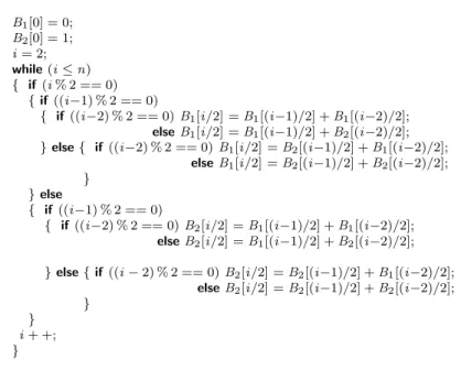
Let us now obfuscate the array by using the rules above. We obtain the program shown in Figure1.1which, after some simplifications, becomes:
B1[0] = 0; B2[0] = 1; i= 2; while(i≤n) {if (i% 2 == 0) B1[i/2] =B2[(i−1)/2] +B1[(i−2)/2]; else B2[i/2] =B1[(i−1)/2] +B2[(i−2)/2]; i+ +; }
B1[0] = 0; B2[0] = 1; i= 2; while(i≤n) { if (i% 2 == 0) {if((i−1) % 2 == 0)
{ if((i−2) % 2 == 0)B1[i/2] =B1[(i−1)/2] +B1[(i−2)/2]; elseB1[i/2] =B1[(i−1)/2] +B2[(i−2)/2];
}else{ if((i−2) % 2 == 0)B1[i/2] =B2[(i−1)/2] +B1[(i−2)/2]; elseB1[i/2] =B2[(i−1)/2] +B2[(i−2)/2];
} }else
{ if((i−1) % 2 == 0)
{ if((i−2) % 2 == 0)B2[i/2] =B1[(i−1)/2] +B1[(i−2)/2]; elseB2[i/2] =B1[(i−1)/2] +B2[(i−2)/2];
}else{if((i−2) % 2 == 0)B2[i/2] =B2[(i−1)/2] +B1[(i−2)/2]; elseB2[i/2] =B2[(i−1)/2] +B2[(i−2)/2];
} } i+ +;
}
Figure 1.1: Fibonacci program after an array split
Simplification was achieved by removing infeasible paths. For instance, if we had
if(i% 2 == 0) { if((i−1) % 2 == 0{X;} else {Y;} }
then we would know that the block of statements X could never be executed, since ifi% 2 = 0 is true then (i−1) % 2 = 0 is false. So, out of the eight possible assignments, we can eliminate six of them.
1.3.8
Array Merging
For another obfuscation, we can the reverse the process of splitting an array by merging two (or more) arrays into one larger array. As with a split, we will need to determine the order of the elements in the new array.
Let us give a simple example of a merge. Suppose we have arraysB1 of size
m1 and B2 of size m2 and a new array A of size m1+m2. We can define a
relationship between the arrays as follows:
A[i] =
B1[i] ifi <m1
B2[i−m1] ifi ≥m1
This transformation is analogous to the concatenation of two sequences (lists).
1.3.9
Other obfuscations
All of the obfuscations that we have discussed so far only consider transforma-tions within methods. Below are some transformatransforma-tions that deal with methods themselves:
• Outlining A sequence of statements within a method is made into a separate method.
• InterleavingTwo methods are merged; to distinguish between the orig-inal methods, an extra parameter could be passed.
• CloningMany copies of the same method are created by applying differ-ent transformations.
1.4
Conclusions
We have seen there is a need for software protection, and code obfuscation is one method for making reverse engineering harder. We have summarised some current obfuscation techniques and highlighted a few of the many commercial obfuscators available. In Section1.2we reviewed two definitions of obfuscation: the definition of Collberget al.[10] uses various complexity metrics and Baraket al.[6] prove that obfuscation is impossible using their definition. We have seen how to apply obfuscations to variables and arrays. In Chapter3we shall develop a different approach to obfuscation which enables us to apply obfuscations to more abstract data structures. As a consequence we will give a new definition for obfuscation and also discuss the efficiency of obfuscated operations.
In the next chapter, we give a case study of a situation where there is a particular need for obfuscation and give specifications for some obfuscations.
Obfuscations for
Intermediate Language
. . . if you stick a Babel fish in your ear you can instantly understand anything said to you in any form of language
The Hitchhiker’s Guide to the Galaxy (1979)
Before we look at a new approach to obfuscation, we present a case study in which we explore a potential application of obfuscation. We look at the inter-mediate language that is part of Microsoft’s .NET platform and we give some obfuscations for this language. In particular, we specify some generalisations of some of the obfuscations given in Section1.3.
2.1
.NET
The heart of Microsoft’s .NET framework is the Common Language Infras-tructure [23] which consists of an intermediate language (IL) which has been designed to be the compilation target for various source languages. IL is a typed stack based language and since it is at quite a high level, it is fairly easy to decompile IL to C# [3]. Two example decompilers are Anakrino [2] and Salamander [45]. IL is similar to Java bytecode but more complicated as it is the compilation target for various languages.
Programs written using .NET are distributed as portable executables (PEs) which are compact representations of IL. These executables are then just-in-time compiled on the target platform. We can translate a PE to IL by using a disassembler and we can convert back by using anassembler. This means that from a PE we can disassemble back to IL and then decompile back to C#. Since we can convert a PE to C#, there is a need for obfuscation.
2.1.1
IL Instructions
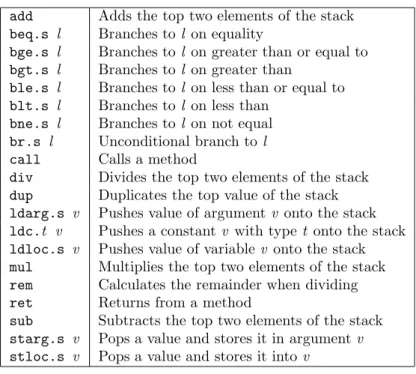
Before we describe some IL obfuscations, we give a brief overview of IL. We concentrate on a fragment of IL — the instructions of interest are shown in
add Adds the top two elements of the stack
beq.s l Branches tol on equality
bge.s l Branches tol on greater than or equal to
bgt.s l Branches tol on greater than
ble.s l Branches tol on less than or equal to
blt.s l Branches tol on less than
bne.s l Branches tol on not equal
br.s l Unconditional branch tol call Calls a method
div Divides the top two elements of the stack
dup Duplicates the top value of the stack
ldarg.s v Pushes value of argumentv onto the stack
ldc.t v Pushes a constantv with typet onto the stack
ldloc.s v Pushes value of variablev onto the stack
mul Multiplies the top two elements of the stack
rem Calculates the remainder when dividing
ret Returns from a method
sub Subtracts the top two elements of the stack
starg.s v Pops a value and stores it in argumentv stloc.s v Pops a value and stores it intov
Figure 2.1: Some common IL instructions
Figure2.1. As an example, consider the following C# method which computes the GCD of two integers:
public static intgcd(inta, int b) { intx =a; inty =b; while(x! =y) if(x <y)y =y−x; else x =x−y; returnx; }
After compiling and disassembling this method, we obtain the IL code shown in Figure2.2.
As IL is a typed stack language, each value handled by the stack must have a type associated with it. For example, int32is the type for 4-byte (32-bit) integers andfloat64for 8-byte real numbers — number types can also be signed or unsigned. Non numeric types include stringandbool.
At the start of a method, various properties of the method are stated. First, the signature of the method is given. In the GCD example, we can see that the method expects two integers and returns one integer as the result. Next, the maximum stack depth in the method is specified by using the .maxstack key-word. If we make any changes to the IL code then we should check whether the maximum stack depth has increased and so must change the value of.maxstack
accordingly. Finally the names and types of any local variables for this method are stated using the.localskeyword.
.method public static int32 gcd(int32 a, int32 b) {
.maxstack 2
.locals (int32 V_0, int32 V_1, int32 V_2) IL0000: ldarg.0 IL0001: stloc.0 IL0002: ldarg.1 IL0003: stloc.1 IL0004: br.s IL0014 IL0006: ldloc.0 IL0007: ldloc.1
IL0008: bge.s IL0010
IL000a: ldloc.1 IL000b: ldloc.0 IL000c: sub IL000d: stloc.1 IL000e: br.s IL0014 } IL0010: ldloc.0 IL0011: ldloc.1 IL0012: sub IL0013: stloc.0 IL0014: ldloc.0 IL0015: ldloc.1
IL0016: bne.un.s IL0006 IL0018: ldloc.0
IL0019: stloc.2
IL001a: br.s IL001c
IL001c: ldloc.2
IL001d: ret
Figure 2.2: IL for a GCD method
In the main body of an IL method, instructions can be preceded by a unique label — typically when using ILDASM (the disassembler distributed with .NET) each instruction has a label of the formIL****. Labels are needed for branch instructions.
A value from the stack can be stored in a local variable, V, by using the instructionstloc.s V and similarly, a value stored in a local variableV can be pushed on the stack using ldloc.s V. If the local variable that is being accessed is one of the first four variables that was declared in this method, then there is a shorter form of stloc and ldloc. Suppose the local variable
were.locals(int32 V, int32 W). Then we could write ldloc.0or stloc.1
instead of ldloc.s Vorstloc.s W, respectively. Values passed to the method are accessed usingldargandstarg. So in the GCD method,ldarg.0loads the value of “a” onto the stack. We use the commandldcto load constants (with the appropriate type) onto the stack. As with ldloc, there is another form of the instruction: we can write ldc.i4.4 instead of ldc.i4 4 for the integers 0..8 (note thati4means a 4-byte integer).
Arithmetic operations, such as addand sub, take values off the stack and then put the result back onto the stack. For instance, in the following sequence:
ldc.i4.7 ldc.i4.2 sub
subwill pop 7 and 2 off the stack and push 5 back.
Branches can either be unconditional (of the formbr) or conditional (such as bne— “jump if not equal to”), which compares values from the stack, and requires a target (corresponding to a label). For a conditional jump, if the condition is true, then the next instruction to be executed will be the one at
the target label, otherwise the next instruction following the branch will be executed.
In this example,
IL0001: ldloc.s V
IL0002: ldc.i4.1
IL0003: bge.s IL0020
IL0004: ...
. . .
IL0020: ...
ifV ≥1 thenIL0020 will be executed next — otherwise, IL0004will be exe-cuted.
When writing IL methods, we require that the code that we produce is verifiable — here are some conditions that must be met for verifiability:
• Stacks must have the same height and contain the same types when control flow paths meet.
• Operations must have the correct number of items on the stack (e.g. for a binary operation there must be at least two elements on the stack). • Operations must receive the type that they expect off the stack
If we have verified code then we can be sure that the code will run safely (e.g.the code will not access memory locations that it not permitted to) and so we must ensure that any obfuscations that we apply produce verifiable code.
2.2
IL obfuscations
Now, we will look at how to perform some obfuscations on IL by manually editing an IL file and assembling this file to make a PE. We look at some of the obfuscations given in [10] and we show how to write them in IL. The aim of performing obfuscations on IL is to make it hard for a decompiler to take a PE and produce C#. Ideally, we would like to stop the decompilation process altogether but at the very least, we should make the resulting code harder to understand.
2.2.1
Variable Transformation
For the first example of obfuscating IL, we show how to perform a simple variable transformation (as outlined in Section 1.3.3). The functions we will use to perform the transformations are:
f = λi.(2i−1)
g = λj.((j + 1)/2)
Assignment of a variable corresponds tostlocand use corresponds toldloc. Using the GCD example given in Figure 2.2, we aim to transform the local
variableV 0. So any occurrences of stloc.0will need to be replaced by: ldc.i4.2 mul ldc.i4.1 sub stloc.0
We replace the instructionldloc.0by:
ldloc.0 ldc.i4.1 add ldc.i4.2 div
Also, we need to change the value of .maxstack to 4 as there are more items to be stored on the stack. After assembling and decompiling, we obtain the following program:
private static intgcd(int a, int b) { intx =a∗2−1; inty =b; while((x+ 1)/2 ! = y) { if((x+ 1)/2<y) {y =y−(x + 1)/2;} else {x = ((x+ 1)/2−y)∗2−1;} } return(i+ 1)/2; }
For this trivial example, only a handful of changes need to be made in the IL. For a larger method which has more uses and definitions or for a complicated transformation, manually editing would be time-consuming. So it would be desirable to automate this process.
2.2.2
Jumping into while loops
C# contains a jump instruction goto which allows a program to jump to a statement marked by the appropriate label. Thegotostatement must be within the scope of the labelled statement. This means that we can jump out of a loop (or a conditional) but not into a loop (or conditional). This ensures that a loop has exactly one entry point (but the loop can have more than one exit by using
breakstatements). This restriction on the use of gotoensures that all the flow graphs are reducible [1, Section 10.4]. Thus, the following program fragment would be illegal in C#: if (P) gotoS1; ... while (G) { . . . S1:. . . . . . }
gcd(int a, int b) { int i; int j; i = a; j = b; if (i * i > 0) {goto IL001a;} else {goto IL0016;}
IL000c: if (i < j) {j -= i; continue;} IL0016: i -= j;
IL001a: if (i == j) {return i;} else {goto IL000c;} }
Figure 2.3: Output from Salamander
However in IL, we are allowed to use branches to jump into loops (while
loops do not, of course, occur in IL — they are achieved by using conditional branches). So, if we insert this kind of jump in IL, we will have a control flow graph which is irreducible and a naive decompiler could produce incorrect C# code. A smarter decompiler could change the while into anif statement that usesgotojumps. As we do not actually want this jump to happen, we use an opaque predicate that is always false.
Let us look at the GCD example in Section 2.1.1again. Suppose that we want to insert the jump:
if((x ∗x)<0) gotoL;
before the while loop whereL is a statement in the loop. So, we need to put instructions in the IL file to create this:
IL0100: ldloc.0 IL0101: ldloc.0 IL0102: mul IL0103: ldc.i4.0
IL0104: blt.s IL0010
The place that we jump to in the IL needs to be chosen carefully — a suitable place in the GCD example would be between the instructions IL0003
andIL0004. We must (obviously) ensure that it does actually jump to a place inside the whileloop. Also, we must ensure that we do not interfere with the depth of the stack (so that we can still verify the program). Figure2.3shows the result of decompiling the resulting executable using the Salamander decompiler [45]. We can see that the whilestatement has been removed and in its place is a more complicated arrangement of ifs andgotos.
This obfuscation as it stands is not very resilient. It is obvious that the conditional x ∗x <0 can never be true and so the jump into the loop never happens.
2.3
Transformation Toolkit
In the last section we saw writing obfuscations for IL involved finding appropri-ate instructions and replacing all occurrences of these instructions by a set of
new instructions. This replacement is an example of arewrite rule[32]:
L⇒R if c
which says that if the condition c is true then we replace each occurrence of
L with R. This form of rewrite rule can be automated and we summarise the transformation toolkit described in [22] to demonstrate one way of specifying obfuscations for IL. This toolkit consists of three main components:
• Arepresentation of IL, calledEIL, which makes specifying transformations easier.
• A newspecification language, calledPath Logic Programming, which al-lows us to specify program transformations on the control flow graph. • Astrategy language with which we can control how the transformations
are applied.
We briefly describe these components (more details can be found in [22]) before specifying some of the generalised obfuscations given in Section1.3.
2.3.1
Path Logic Programming
Path Logic Programming (PLP) is a new language developed for the specifica-tion of program transformaspecifica-tions. PLP extends Prolog [51] with new primitives to help express the side conditions of transformations. The Prolog program will be interpreted relative to the flow graph of the object program that is being transformed. One new primitive is
all Q (N,M)
which is true ifN andM are nodes in the flow graph, and all paths fromN to
M are of the form specified by the patternQ. Furthermore, there should be at least one path that satisfies the patternQ. This is to stop a situation where we do not have a path betweenN and M and so the predicateall Q (N,M) will be vacuously true. Similarly, the predicate
exists Q (N,M)
is true if there exists a path fromN toM which satisfies the patternQ. As an example ofall, consider:
all ({ }∗; {0set(X,A), local(X)}; {not(0def(X))}∗; {0use(X)} ) (entry,N)
This definition says that all paths from the program entry to node N should satisfy a particular pattern. A path is a sequence of edges in the flow graph. The pattern for a path is a regular expression and in the above example the regular expression consists of four components:
• Initially we have zero or more edges that we do not particularly care about which is indicated by{ }∗ — the interpretation of{ }is a predicate that is always true.
• Next, we require an edge whose target node is an expression of the form
X :=AwhereX is local variable.
• Then we want zero or more edges to nodes that do not re-defineX. • Finally we reach an edge pointing to nodeN which uses variableX. A pattern, which denotes an property on the control flow graph, is a regular expression whose alphabet is given by temporal goals — the operator ; represents sequential composition, + represents choice, ∗ is zero or more occurrences and
an empty path. A temporal goal is a list of temporal predicates, enclosed in curly brackets. A temporal predicate is either an ordinary predicate (like local in the example we just examined), or a ticked predicate (likeuse). Ticked predicates are properties involving edges and are denoted by the use of a tick mark (0) in front of the predicate. For example, def(X,E) is a predicate that takes two arguments: a variableX and an edgeE, and it holds true when the edge points at a node whereX is assigned. Similarly, use(X,E) is true when the target of E is a node that is labelled with a statement that makes use of
X. When we place a tick mark in front of a predicate inside a path pattern, the current edge is added as a final parameter when the predicate is called.
We can think of the path patterns in the usual way as automata, where the edges are labelled with temporal goals. In turn, a temporal goal is interpreted as a property of an edge in the flow graph. The pattern
{p0,p1, . . . ,pk−1}
holds at edge e if each of its constituents holds at edgee. To check whether a ticked predicate holds at e, we simply add e as a parameter to the given predicate and non-ticked predicates ignoree. A syntax for this language and a more detail discussion ofall andexists is given in [22].
2.3.2
Expression IL
Since IL is a stack based language, performing a simple variable transformation described in Section2.2.1leads to performing quite a complicated replacement. To make specifying transformation easier we work with a representation of IL which replaces stack-based computations with expressions — this representation is called Expression IL(EIL). To convert from IL to EIL, we introduce a new local variable for each stack location and replace each IL instruction with an assignment. As we use only verifiable IL, this translation is possible.
EIL is analogous to both the Jimple and Grimp languages from the SOOT framework [53,54] — the initial translation produces code similar to the three-address code of Jimple, and assignment merging leaves us with proper expres-sions like those of Grimp.
stmt::=nop|var :=exp|br target|brif cnd target exp::=var|const|monop(exp)|binop(exp,exp)
monop::=neg
binop::=add|sub|mul|div|rem
var::=local(name)|arg(name)|local(name)[exp] const::=ldc.type val
cnd::=and(cnd,cnd)|or(cnd,cnd)|not(cnd)|ceq(exp,exp)|cne(exp,exp) |clt(exp,exp)|cle(exp,exp)|cgt(exp,exp)|cge(exp,exp)
target::=string name::=string type::=i4|i8
instr::= [target:]stmt prog::=instr list
Figure 2.4: Syntax for a simple subset of EIL Thus, the following set of IL instructions:
ldc.i4.2 stloc x ldc.i4.3 ldloc x add stloc y
is converted to something like:
local(v1) := ldc.i4.2
local(x) := local(v1)
local(v2) := ldc.i4.3 local(v3) := local(x)
local(v4) := add(local(v2), local(v3))
local(y) := local(v4)
We can then perform standard compiler optimisations (such as constant prop-agation and dead code elimination) to simplify this set of instructions further. We concentrate on only a simple fragment of EIL and a concrete syntax for this fragment is given in Figure2.4.
This concrete syntax omits many significant details of EIL; for example, all expressions are typed and arithmetic operators have multiple versions with different overflow handling. This detail is reflected in the representation of these expressions as logic terms. For example, the integer 5 becomes the logic term
expr type(ldc(int(true,b32),5),int(true,b32))
The first parameter of expr type is the expression and the second is the type — this constructor reflects the fact that all expressions are typed. The type
int(true,b32) is a 32-bit signed integer (thetruewould becomefalseif we wanted an unsigned one). To construct a constant literal, the constructor ldc is used — it takes a type parameter, which is redundant but simplifies the processing of EIL in other parts of the transformation system, and the literal value.
For a slightly more complicated example, the expressionx+ 5 (wherex is a local variable) is represented by
expr type(applyatom(add(false,true),
expr type(localvar(sname(“x”)),
int(true,b32)),
expr type(ldc(int(true,b32),5),
int(true,b32))),
int(true,b32))
The term localvar(sname(“x”)) refers to the local variablex — the seemingly redundant constructor sname reflects the fact that it is also possible to use a different constructor to refer to local variables by their position in the method’s declaration list, although this facility is not used.
The constructor applyatom exists to simplify the relationship between IL and EIL — the termadd(false,true) directly corresponds to the IL instruction
add, which adds the top two items on the stack as signed values without over-flow. Thus, the meaning of applyatom can be summarised as: “apply the IL instruction in the first parameter to the rest of the parameters, as if they were on the stack”.
Finally, it remains to explain how EILinstructionsare defined. It is these that will be used to label the edges and nodes of flow graphs. An instruction is either an expression, a branch or a return statement, combined with a list of labels for that statement using the constructorinstr label. For example, the following defines a conditional branch to the label target:
instr label(“conditional” :nil,
branch(cond(. . .),“target”))
Note that we borrow the notation for lists from functional programming, writing
X :Xs instead of [X|Xs]. If the current instruction is an expression, thenexp
enclosing an expression would be used in place ofbranch, and similarlyreturn
is used in the case of a return statement.
2.3.3
Predicates for EIL
The nodes of the flow graph are labelled with the logic term corresponding to the EIL instruction at that node. In addition, each edge is labelled with the term of the EIL instruction at the node that the edge points to; it is these labels that are used to solve the existential and universal queries.
The logic language provides primitives to access the relevant label given a node or an edge — @elabel(E,I) holds if I is the instruction at edge E, and @vlabel(V,I) holds if I is the instruction at node V (where @ denotes a primitive).
We can define theset predicate used in Section2.3.1as follows:
set(X,A,E) :−
@elabel(E,instr label( ,exp(expr type(assign(X,A), )))).
Note that we denote unbound variables by using an underscore. It is straight-forward to definedef in terms ofset:
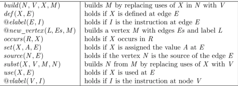
build(N,V,X,M) buildsM by replacing uses ofX inN withV def(X,E) holds ifX is defined at edgeE
@elabel(E,I) holds ifI is the instruction at edgeE
@new vertex(L,Es,M) builds a vertexM with edgesEs and labelL occurs(R,X) holds ifX occurs inR
set(X,A,E) holds ifX is assigned the valueA atE
source(N,E) holds if the vertexN is the source of the edge E subst(X,V,M,N) buildsN from M by replacing uses ofX withV use(X,E) holds ifX is used atE
@vlabel(V,I) holds ifI is the instruction at nodeV
Figure 2.5: Some common predicates
The definition of use is based on the predicate occurs(R,X), which checks whether X occurs in R (by the obvious recursive traversal). When defining
use(X,E), we want to distinguishuses ofX from definitions ofX, whilst still finding the uses of the variablex in expressions such asa[x] := 5 andx :=x+ 1:
use(X,E):−@elabel(E,S),occurs(S,X),
not(def(X,E)).
use(X,E):−set( ,R,E),occurs(R,X).
The common predicates that we will use are summarised in Figure2.5.
2.3.4
Modifying the graph
When creating new vertices the predicatebuild will often be used. The expres-sion build(N,V,X,M) creates a new vertexM, by copying the old vertexN, replacing uses ofX withV:
build(N,V,X,M) :−@vlabel(N,Old),
subst(V,X,Old,New),
listof(E,source(N,E),Es),
@new vertex(New,Es,M).
The predicate:
subst(V,X,Old,New)
constructs the termNew from Old, replacing uses ofV withX. As withuse, it is defined so as not to apply this todefinitions ofX — if we are replacingx
with 0 inx :=x+ 1 we want to end up withx := 0 + 1, not 0 := 0 + 1. New vertices are constructed by using @new vertex. This primitive takes a vertex label and a list of outgoing edges and binds the new vertex to its final parameter. For the definition of build we use the same list of edges as the old vertex, since all we wish to do is to replace the label.
The predicatesource(N,E) is true if the vertexN is the source of the edge
E, whilst thelistof predicate is the standard Prolog predicate which takes three parameters: a termT, a predicate involving the free variables ofT, and a third parameter which will be bound to a list of all instantiations ofT that solve the predicate. Thus the overall effect oflistof(E,source(N,E),Es) is to bindEsto the outgoing edges from nodeN, as required.
2.3.5
Applying transformations
Although the logic language we have described makes it convenient to define side conditions for program transformation, it would be rather difficult to use this language to apply these transformations, since that would require the pro-gram flow graph to be represented as a logic term. The approach that is taken is that a successful logic query should also bind its parameter to a list of symbolic “actions” which define a correct transformation on the flow graph. A high-level strategy language, which is similar to Stratego [55], is responsible for direct-ing in what order logic queries should be tried and for applydirect-ing the resultdirect-ing transformations.
An action is a term, which can be either of the formreplace vertex(V,W) ornew local(T,N). The former replaces the vertexV with the vertexW, while the latter introduces a new local variable namedN of typeT. We write a list of actions as the last parameter of predicate.
Suppose that we have a predicate P specified. If we want to apply this predicate once then we writeapply(P) in the strategy language. If we want to exhaustively apply this predicate (i.e. keep applying the predicate while it is true) then we writeexhaustively(apply(P)). An example of a strategy is given at the end of the next section.
2.3.6
Variable Transformation
For our first example, let us consider how to define a variable transformation (Section 1.3.3). The first part of the transformation involves finding a suitable variable and for simplicity, we require that the variable is local and has integer type. We also require that it is assigned somewhere (otherwise there would be no point in performing the transformation). Once we find a suitable variable (which we call OldVar), we generate a new name using @fresh name which takes a type as a parameter. We can write the search for a suitable variable as follows:
find local(OldVar,
NewVar,
new local(int(true,b32),NewVarName) :nil
) :−
exists({ }∗;
{0set(OldVar,V),
OldVar =expr type(localvar( ),int(true,b32))} ) (entry,OldVarVert),
@fresh name(int(true,b32),NewVarName),
NewVar=expr type(localvar(sname(NewVarName)),
int(true,b32)).
The next step of the transformation replaces uses and assignments ofOldVar
exhaustively. To do this, we need to define predicates which allow us to build expressions corresponding tof and g (the functions used for variable transfor-mation). The predicateuse fn(A,B) binds B to a representation ofg(A) and similarly,assign fn(C,D) bindsD tof(C). We can specify any variable trans-formation by changing these two predicates. As an example, let us suppose
that
f = λi.(2i)
g = λj.(j/2) Then we would define
use fn(A,
expr type(applyatom(cdiv(true),
A,
expr type(applyatom(ldc(int(true,b32),2)),
int(true,b32))),
int(true,b32))).
and we can defineassign fn similarly.
We define a predicatereplace varwhich replaces occurrences ofOldVarwith
NewVar with the appropriate transformation. We need to deal with assignment and uses separately. We can easily write a predicate to replace uses ofOldVar
as follows:
replace var(OldVar,
NewVar,
replace vertex(OldVert,NewVert) :nil
) :−
exists({ }∗;
{0use(OldVar)} ) (entry,OldVert),
use fn(NewVar,NewUse),
build(OldVert,NewUse,OldVar,NewVert).
To replace assignments toOldVar we cannot use thebuild and instead have to create a new vertex manually — the definition is shown in Figure 2.6. In this definition, we use the predicatesetto find a vertex where there is an assignment of the form OldVar:=OldVal. At this vertex, we find a list of edges from this vertex and the list of labels. We then create the expressionf(OldVal) and bind it toNewVal. Finally, we use the predicatebuild assign to create a new vertex that contains the instructionNewVar :=NewVal and which has the same labels and edges asOldVar.
To apply this transformation, we write the following two lines in the strategy language:
apply(find local(OldVar,NewVar));
exhaustively(apply(replace var(OldVar,NewVar)))
The first line applies the search to find a suitable variable and the second ex-haustively replaces all occurrences of the old variable with the new variable.
2.3.7
Array Splitting
For our second example, we consider splitting an array using the method stated in Section1.3.6. First, we briefly describe how to find a suitable array — more details can be found in [22].
replace var(OldVar,
NewVar,
replace vertex(OldVert,NewVert) :nil
) :−
exists({ }∗;
{0set(OldVar,OldVal)} ) (entry,OldVert),
listof(OldEdge,source(OldVert,OldEdge),OldEdges),
@vlabel(OldVert,instr label(Labels, )),
assign fn(OldVal,NewVal),
build assign(Labels,NewVar,NewVal,OldEdges,NewVert).
build assign(Labs,L,R,Edges,Vert) :−
@new vertex(instr label(Labs,exp(expr type(assign(L,R),
int(true,b32)))),
Edges,Vert).
Figure 2.6: Predicates for replacing assignments Finding a suitable array
We need to find a vertexInitVert which has an array initialisation of the form:
OldArray:=newarr(Type)[Size]
whereOldArray is a local variable of array type.
For this transformation to be applicable, we ensure that every path through our method goes through InitVert and that the array is always used with its index (except at the initialisation) — so for example, we cannot pass the whole array to another method. We can write this safety condition as follows:
safe to transform(InitVert,OldArray) :−
all({ }∗;
{ 0isnode(InitVert)};
{ not(0unindexed(OldArray))}∗ ) (entry,exit).
The predicate unindexed(OldArray,E) holds if OldArray is used without an index at the node pointed to by edge E. We define unindexed by pattern matching to EIL expressions. So, for example:
unindexed(A,A).
unindexed(exp(E),A) :− unindexed(E,A).
unindexed(expr type(E,T),A) :− unindexed(E,A).
unindexed(arrayindex(L,R),A) :− not(L=A), unindexed(L,A).
unindexed(arrayindex(L,R),A) :− unindexed(R,A).
After a suitable array has been found we need to create initialisations for our two new arrays with the correct sizes.
replace array(A,B1,B2,replace vertex(N,M) :nil) :−
exists({ } ∗; {0set(X,V),
X =expr type(arrayindex(A,I), )} ) (entry,N),
listof(E,source(N,E),Es),
@vlabel(N,instr label(L, )),
is even(I,C),
index(I,J),
@fresh label(ThenLab),
build assign(ThenLab:nil,
expr type(arrayindex(B1,J),int(true,b32)),
V,Es,ThenVert),
new edge(ThenVert,ThenEdge),
@fresh label(ElseLab),
build assign(ElseLab:nil,
expr type(arrayindex(B2,J),int(true,b32)),
V,Es,ElseVert),
new edge(ElseVert,ElseEdge),
@new vertex(instr label(L,branch(cond(C),ThenLab)),
ThenEdge:ElseEdge:nil,M).
Figure 2.7: Definition ofreplace array for assignments Replacing the array
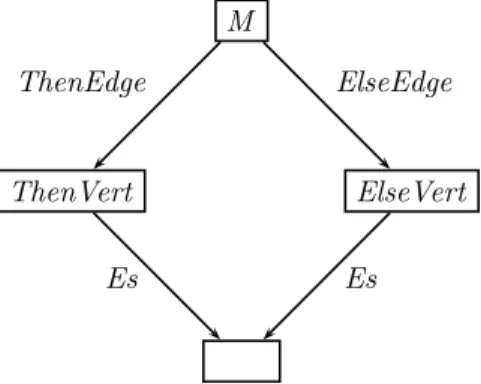
Once we have identified which array we want to split (and checked that it is safe to do so) then we need to replace exhaustively the original array with our two new ones. As with variable transformation, we have to treat uses and assignments of array values separately. But instead of a straightforward substitution, we have to insert a conditional expression at every occurrence of the original array.
Let us consider how we can replace an assignment of an array value. Suppose that we want to split an array A into two arrays B1 and B2 using the split
(Equation (1.4)) defined in Section 1.3.6. For an assignment of A, we look for a statement of the form:
A[I] =V
and, from Equation (1.5), we need to replace it with a statement of the form:
if((i%2) == 0) {B1[i/2] =V;} else {B2[i/2] =V;}
The predicate for this transformation is given in Figure2.7. The first step in the transformation is to find an assignment toAby using the predicateset. We want to match the left-hand side of an assignment to
expr type(arrayindex(A,I),T)
where I is the index of the array (andT is the type). Once we find the node,
N, of such an assignment, we need to find the list of outgoing edges fromN and the labelLforN.
M
ThenVert ElseVert
ThenEdge ElseEdge
Es Es
Figure 2.8: Flow graph to build a conditional expression
Next, we create a testC corresponding to i% 2 == 0 in the the predicate
is even(I,C) and we create an expressionJ for the indices of the new arrays, using the predicateindex(I,J) (we omit the details of these predicates).
Now, we need to create vertices corresponding to the branches of the con-ditional — the flow graph we want to create is shown in Figure 2.8. To create the “then” branch, we first obtain a fresh labelThenLab with which we create a new vertexThenVert. This vertex needs to contain an instructionB1[J] =V
and have the same outgoing edges asN. Then we create a new incoming edge,
ThenEdge, forThenVert. The construction of the “else” branch is similar (we build the instructionB2[J] =V instead).
Finally, we are ready to build a new vertexM which replacesN. This vertex contains an instruction for the conditional which has labelL. The outgoing edges for this vertex areThenEdge andElseEdge.
Replacing uses of the original array is slightly easier. Instead of manually buildingThenVert andElseVert we can use the predicatesubst to replaceA[I] withB1[J] orB2[J] as appropriate.
We can adapt this specification for other array splits. In Section1.3.6, we defined an array split in terms of three functions ch, f1 and f2. The predicate
is even corresponds to the function ch and index corresponds to f1 and f2
(which are equal for our example). So by defining a predicate that represents
ch and two predicates forf1 and f2, we can write a specification for any split
that creates two new arrays.
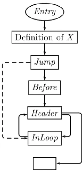
2.3.8
Creating an irreducible flow graph
In Section2.2.2, we saw how by placing anif statement before a loop we could create a method with an irreducible control flow graph. Could we specify this transformation in PLP? The control flow graph that we want to search for is shown in Figure 2.9 and we would like to place a jump from the node Jump
to the node InLoop. However, in EIL (and IL) we do not have an instruction corresponding towhile; instead we have to identify a loop from the flow graph. Figure 2.10 contains the logic program that performs this transformation. The code has two parts: the first finds a suitable loop and the second builds the jump.