On the Validity of Minimin and Minimax Methods for
Support Vector Regression with Interval Data
Andrea Wiencierz Department of Mathematics University of York [email protected] Marco E. G. V. Cattaneo Department of Mathematics University of Hull [email protected]
Abstract
In the recent years, generalizations of support vec-tor methods for analyzing interval-valued data have been suggested in both the regression and classifica-tion contexts. Standard Support Vector methods for precise data formalize these statistical problems as optimization problems that can be based on various loss functions. In the case of Support Vector Regres-sion (SVR), on which we focus here, the function that best describes the relationship between a response and some explanatory variables is derived as the solution of the minimization problem associated with the ex-pectation of some function of the residual, which is called the risk functional. The key idea of SVR is that even when considering an infinite-dimensional space of arbitrary regression functions, given a finite-dimensional data set, the function minimizing the risk can be represented as the finite weighted sum of kernel functions. This allows to practically determine the SVR estimate by solving a much simpler optimization problem, even in the case of nonlinear regression. In case that only interval-valued observations of the vari-ables of interest are available, it has been suggested to minimize the minimal or maximal risk values that are compatible with the imprecise data, yielding precise SVR estimates on the basis of interval data. In this pa-per, we show that also in the case of an interval-valued response the optimal function can be represented as the finite weighted sum of kernel functions. Thus, the minimin and minimax SVR estimates can be obtained by minimizing the corresponding simplified expressions of the empirical lower and upper risks, respectively. Keywords. Support Vector Regression, interval data, Representer Theorem.
1 Introduction
In this paper, we deal with the generalization of Sup-port Vector Regression (SVR) to interval data. By SVR we denote a class of kernel-based methods for
the statistical problem of regression analysis. These methods originated in the field of Machine Learning (Vapnik, 1998, 1995) and recently also gained attention in the field of Statistics (see, e.g., Hable, 2012; Christ-mann et al., 2009; HofChrist-mann et al., 2008; Steinwart and Christmann, 2008). The typical goal of a regres-sion analysis is to describe the relationship between a response variableY ∈ Y ⊆Rand a numberd∈N of explanatory variables X ∈ X ⊆Rd by a function f : X → R. The sought-after function f is usually assumed to be a member of a particular space F of
considered regression functions, for example, the space of all (affine) linear functions.
To identify which functions in F best describe the
relationship between the random variables in (X, Y) = V, the considered regression functions are assessed by a loss function. Most common loss functions are characteristics of the distribution of (some function of) the residualRf, which we here define by
Rf =|Y −f(X)|
for eachf ∈ F. In the SVR methodology, the
expecta-tion of some usually convex error funcexpecta-tion is considered as loss function, which is called risk functional. If the probability distributionPV of the random vectorV is known, the distribution ofRf can be derived from it and the best regression functions can be identified by minimizing the chosen loss function. Yet, usually the true distribution of the investigated variables is un-known, but it is assumed thatPV lies in some specific set of probability measuresPV. Thus, the evaluation of each regression function also varies over possible distributions of V.
Given the realization of an independent sample of ran-dom variables V1 = (x1, y1), . . . , Vn = (xn, yn), with
n∈N, where Vi ∼PV for alli∈ {1, . . . , n}, we can
learn something about the distribution of the variables of interest. In SVR, the empirical distribution ˆPV of the observations is used as a point estimate ofPV and the (regularized) risk under this particular
distribu-tion is minimized to obtain the regression estimate. The SVR estimate is in general unique. Moreover, the so-called Representer Theorem states that the func-tion minimizing the risk given the observafunc-tions can be represented as the finite weighted sum of kernel functions. This is a key result for SVR, as it allows to practically determine the SVR estimate by solving a relatively simple optimization problem, even in the case of nonlinear regression. Further details of the SVR methodology are presented in the next section. If the variables of interest are not observed as pre-cise numbers but only upper and lower bounds to the values are available, the empirical distribution ˆPV is not revealed by the observable data. We denote the random sets describing the observables byV∗
1, . . . , Vn∗ and their probability distribution byPV∗. If the
ob-served intervals are assumed to cover the unknown precise values with probability one, bounds for the empirical risk can be derived from the empirical dis-tribution ˆPV∗ of the imprecise data. How can we use
this information to obtain an SVR estimate in this situation? Starting from the simplified representation of the optimal function in standard SVR, Utkin and Coolen (2011) proposed to follow a minimin or a mini-max approach and to minimize either the lower or the upper (regularized) risk in order to obtain a precise regression estimate.
In this paper, we investigate the validity of their start-ing from the simplified representation in the general-ized data situation. At first, we introduce the formal framework of the SVR methodology in detail and for-mally discuss Utkin and Coolen (2011)’s SVR general-ization. Then, we consider the Representer Theorem in the more general data situation. We find that also in this case the optimal function can be represented as the finite weighted sum of kernel functions. Finally, after applying the discussed SVR methods to an in-teresting problem in the area of winemaking, a short outlook concludes the paper.
2 Methodological Framework of SVR
In this section, the formal framework of SVR with precise data is presented. In the SVR methodology, the setPV is assumed to contain all probability measures onV=X × Y. In this paper, we additionally assumethatYis a bounded subset ofR. Furthermore, in SVR, the loss assigned to a possible regression function f and a distributionPV is the riskEPV(f). Presupposing measurability, the risk functional EPV on F can be defined for eachPV ∈ PV as
EPV : f 7→ EPV(f) =EPV(ψ(Rf)), (1)
where ψ is a convex mapping fromR≥0 toR≥0
sat-isfying ψ(0) = 0 and EPV denotes the expectation with respect toPV. For example, if ψis defined by ψ(r) =r2for allr∈R≥0, the loss associated with a
pair (f, PV) is given byEPV(f) =EPV(R2f). Thus, we obtain the loss function corresponding to Least Squares regression. Another famous example is the function defined by ψ(r) = max{0, r−ν}, for allr∈R≥0 and
some ν ≥0, which was introduced by Vapnik (1995,
Section 6.1) and represents the so-called ν-insensitive loss.
The convexity of the mappingψimplies convexity of the risk functional EPV, that is, the risk functional satisfies for eachρ∈[0,1]
EPV (ρ f+ (1−ρ)f
′)≤ρE
PV(f) + (1−ρ)EPV(f
′),
for allf, f′ ∈ F (see also Steinwart and Christmann,
2008, Lemma 2.13). As explained later, this property is crucial to the existence of a unique optimal regression function.
In the SVR framework, the space F of considered
regression functions from X to R is supposed to be a Reproducing Kernel Hilbert Space (RKHS) with associated scalar product ⟨·,·⟩F : F → R.
An RKHS is uniquely associated with its repro-ducing kernel function. A kernel function κ is a positive semi-definite function on X × X, that is,
Pn i=1
Pn
j=1αiαjκ(xi, xj)≥0, for allα1, . . . , αn∈R, x1, . . . , xn ∈ X, and n ∈N. Here, we only consider kernel functions that are moreover measurable and bounded. If κ is the reproducing kernel function of the RKHSF, for eachx∈ X we have κ(·, x)∈ F and
f(x) =⟨f, κ(·, x)⟩F,
for allf ∈ F. From this property called reproducing
property follows thatκ(x, x′) =⟨κ(·, x), κ(·, x′)⟩ F, for
all x, x′ ∈ X. A simple example for an RKHS and
its reproducing kernel is the function space associated with the linear kernel defined byκ(x, x′) =⟨x, x′⟩+ 1,
for all x, x′ ∈ X, which is the Hilbert space of all
(affine) linear functions fromXtoR. Another common kernel function is the so-called Gaussian kernel, which is defined for allx, x′ ∈ X by
κ(x, x′) = exp −1
σ2∥x−x′∥
2,
with σ > 0. The associated RKHS is a very large function space that is dense in the space of all continu-ous (real-valued) functions onX. For more details on kernels and RKHSs, see, for example, Steinwart and Christmann (2008, Chapter 4).
To avoid obtaining too wiggly functions as descriptions of the relationship of interest when the regression analysis is based on a finite sample of observations,
the risk is further supplemented by an additive penalty for the complexity of the functionsf ∈ F. Hence, in the SVR methodology, instead ofEPV the regularized risk functionalEPV,λ is minimized, which is defined for allf ∈ F by
EPV,λ(f) =EPV(f) +λ∥f∥ 2
F,
where λ >0 is a fixed parameter regulating the penal-ization and∥ · ∥F is the norm induced by the scalar
product inF. The regularization can be interpreted
as minimizingEPV under the restriction∥f∥2F≤c, for some c ∈R≥0, but instead of choosing the bound c
explicitly, we fix the value of the corresponding La-grange multiplier λin the constrained optimization problem.
As the functional f 7→ λ∥f∥2F is strictly convex by
general properties of norms andEPV is convex because ofψ, we have thatEPV,λis also a strictly convex func-tional onF. Exploiting the strict convexity ofEPV,λ, it can be shown that an optimal function always exists and is unique, provided that some regularity condi-tions are fulfilled (see, e.g., Steinwart and Christmann, 2008, Lemma 5.1 and Theorem 5.2).
Given observations (x1, y1), . . . ,(xn, yn) of an
inde-pendent and identically distributed random sample V1, . . . , Vn, the SVR methodology consists in estimat-ingPV by the corresponding empirical distribution ˆPV, before identifying the regression estimatefPˆV,λ∈ Fby the minimization ofEPˆV,λ, for someλ >0. Like in the general case, there always exists a unique minimizer of the regularized risk for ˆPV. Moreover, the so-called Representer Theorem states that this unique function fPˆV,λcan be represented as the linear combination of the corresponding functionsκ(·, x1), . . . , κ(·, xn), that
is, there exist weightsα1, . . . , αn∈Rsuch that fPˆV,λ(x) =
n X j=1
αjκ(x, xj), (2) for all x∈ X (see, e.g., Steinwart and Christmann, 2008, Theorem 5.5). This expression is sometimes called support vector expansion offPˆV,λand the op-timal functionfPˆV,λ is often referred to as a Support Vector Machine (SVM). This term can be explained historically, because Vapnik (1998, 1995) proposed to use functions forψthat have the property that some of the resultingα1, . . . , αn are zero. The vectorsxjfor
whichαj̸= 0 are called support vectors, whence the notion SVM. One example for such a representing func-tionψis the function associated with theν-insensitive loss mentioned before. Nevertheless, in general, SVMs are not sparse in this sense (see, e.g., Steinwart and Christmann, 2008, Section 11.1).
The result of the Representer Theorem expressed in (2) is extremely useful for the practical computation
of SVR estimates as it simplifies the associated op-timization problems and allows to solve them even when large RKHSs of arbitrary smooth regression functions are considered, like, for example, the RKHS associated with the Gaussian kernel. Given a data set (x1, y1), . . . ,(xn, yn) with empirical distribution
ˆ
PV and a fixedλ >0, Equation (2) tells us thatfPˆV,λ is an element of the setFn⊂ F, with
Fn = Xn j=1 αjκ(·, xj) : α1, . . . , αn∈R .
Furthermore, for all functions fα=Pnj=1αjκ(·, xj), with α = (α1, . . . , αn)T ∈ Rn, the squared norm is
given by ∥fα∥2F =Pni=1Pnj=1αiαjκ(xi, xj). Hence, the regularized risk associated with ˆPV can be written for eachfα∈ Fn as EPˆV,λ(fα) = 1 n n X i=1 ψ yi−Pnj=1αjκ(xi, xj) +λ n X i=1 n X j=1 αiαjκ(xi, xj).
AsEPˆV,λis convex, the SVMfPˆV,λcan be obtained by solving a convex optimization problem over α∈Rn, for which there are numerous efficient algorithms (see, e.g., Boyd and Vandenberghe, 2004). For the selection of an appropriate regularization parameterλ >0 and of other hyper-parameters like the parameter σof the Gaussian kernel, different strategies can be applied, for instance, cross-validation (see, e.g., Steinwart and Christmann, 2008, Section 11.3). Since we are mainly interested in the generalization of a key theoretical result about SVR to the situation with interval data, we neglect the latter issues in this paper and always consider these parameters fixed.
3 SVR with Interval Data
In this section, we investigate whether the SVR methodology can be used for regression analysis when the variables of interest cannot be observed as precise numbers but only (bounded) intervals covering the val-ues of interest are available. Utkin and Coolen (2011) proposed a generalization of the SVR methodology to this situation. As we will see later, the suggested methods of Utkin and Coolen (2011) work well for interval-valued observations of the response variable Y, but cannot directly be extended to interval-valued observations of the variables inX. Therefore, we also consider here only the situation where instead of V the random setV∗∈ V∗⊆2V is observed, whose
pos-sible realizations are of the form {X} ×[Y , Y], with
3.1 Utkin and Coolen (2011)’s SVR Generalization
Now, we discuss the generalization of SVR proposed by Utkin and Coolen (2011) in detail. Since in the considered data situation the precise variables are not observable, it is impossible to evaluate the considered regression functions f ∈ F by EPˆV(f), i.e., by the risk associated with the empirical distribution of the precise data. However, the probability distribution of the imprecise dataPV∗ can be estimated on the basis
of the observations.
When the probability distribution PV∗ of the
observ-able data is known, as we assume that the interval [Y , Y] covers the precise unobservableY with proba-bility one, we know that the unknown probaproba-bility dis-tribution of the precise data lies in the set [PV∗]⊆ PV containing all distributions of the precise data, PV, that satisfy for all measurable events A⊆ V the in-equalities
PV(V ∈A)≥PV∗(V∗⊆A) and
PV(V ∈A)≤PV∗(V∗∩A̸=∅).
(3)
By consequence, for all f ∈ F, the unknown risk
EPV(f) lies in the interval [EPV∗(f),EPV∗(f)], where
EPV∗(f) = min P′ V∈[PV∗] EP′ V(f) and EPV∗(f) = max P′ V∈[PV∗]EP ′ V(f).
Hence, in the regression problem with interval-valued response, the set [EPV∗(f),EPV∗(f)] of all possible risk values constitutes the loss evaluation for each f ∈ F. Of course, it is in general impossible to directly
determine an optimal function with respect to this imprecise criterion. The central idea of the regression methodology proposed by Utkin and Coolen (2011) is to use the minimin or the minimax rule to solve this problem, that is, to minimize either the lower risk
EPV∗ or the upper risk EPV∗ in order to identify a
single optimal regression function.
To derive expressions of the lower and upper risks, Utkin and Coolen (2011) describe, for each regression functionf ∈ F, the set of compatible probability dis-tributions of the residualRf given PV∗ by a so-called
p-box and apply results from Utkin and Destercke (2009). Introduced by Ferson et al. (2003, Section 2), the notion p-box designates a convex set of probabil-ity measures for a univariate random quantprobabil-ity that is bounded by a lower and an upper cumulative distribu-tion funcdistribu-tion. In the situadistribu-tion considered here, given PV∗, also the marginal distribution of the
interval-valued residual [Rf, Rf], where Rf = min
(x,y)∈V∗|y−f(x)| and
Rf = max
(x,y)∈V∗|y−f(x)|,
is known for each f ∈ F. According to (3), the marginal distribution of the imprecise residual im-plies lower and upper bounds to the probabilities of all measurable events associated with the marginal distribution of the precise residual Rf. If we consider these lower and upper bounds for all events of the form (−∞, r], with r∈ R≥0, we obtain a lower and
an upper cumulative distribution function that con-stitute a p-box. As the p-box covers all probability distributions of Rf that comply with the bounds at least for the intervals (−∞, r], withr∈R≥0, some of
the probability measures included in the p-box may not satisfy (3) for all measurable events, and thus, may be incompatible with the marginal distribution of the imprecise residual. However, the p-box obtained in the described way from the random set [Rf, Rf], withf ∈ F, is the tightest outer approximation by a p-box of the set of probability distributions of Rf implied by this random set (see, e.g., Destercke et al., 2008). In fact, in the present situation, for eachf ∈ F, the upper bound of the associated p-box corresponds to the cumulative distribution function of the lower endpoint of the interval-valued residual [Rf, Rf], while the lower bound of the p-box corresponds to the cu-mulative distribution function of the upper endpoint. This can be seen by considering the corresponding bounds to the probabilities of the events (−∞, r], with
r∈R≥0, used to derive the p-box for allf ∈ F, that
is,
PV(Rf ≤r)≥PV∗([Rf, Rf]⊆(−∞, r]) and
PV(Rf ≤r)≤PV∗([Rf, Rf]∩(−∞, r]̸=∅)
It can easily be checked that the probability distribu-tions corresponding to the bounds of the p-box comply with (3) for arbitrary measurable events, and thus, are elements of [PV∗]. Since, according to its definition
in (1), the risk functional EPV is the expectation of a convex function in Rf with minimum at zero, it is straightforward to conclude that EPV∗ and EPV∗
coincide with the expected errors associated with the marginal distributions of the lower and of the upper residual, that is, of Rf and ofRf, respectively (see also Utkin and Destercke, 2009, Proposition 3). Now consider that the realization of an independent sample of random sets V1∗=A1, . . . , Vn∗ =An is ob-served, whereVi∗ ∼PV∗ for alli∈ {1, . . . , n}. Then, by analogy with standard SVR, PV∗ is estimated by
and furthermore, the complexity of the estimated func-tions is restricted by an additive penalty term. Hence, the optimization criteria considered in the minimin and minimax generalizations of SVR are the regular-ized lower and upper risk, respectively. For a fixed penalization parameter λ >0, the regularized lower and upper risks associated with the empirical distribu-tion ˆPV∗ can, for eachf ∈ F, be expressed as follows:
EPˆV∗,λ(f) = 1 n n X i=1 min (xi,yi)∈Ai ψ(|yi−f(xi)|) +λ∥f∥2F, EPˆV∗,λ(f) = 1 n n X i=1 max (xi,yi)∈Ai ψ(|yi−f(xi)|) +λ∥f∥2F, (4) where ψ is again the convex mapping from R≥0 to
R≥0 representing the chosen loss.
Utkin and Coolen (2011) deduce from these expres-sions of the regularized empirical lower and upper risks solvable formulations of the optimization problems cor-responding to both suggested strategies in the special case of linear regression for different choices of the loss function. We do not restrict the approach to this special case here and continue to consider more general RKHSs of regression functions. Moreover, Utkin and Coolen (2011) start from the support vector expan-sion (2) of the solution of the optimization problem corresponding to standard SVR. However, it first has to be verified that the Representer Theorem applies to or that its statements can be transferred to the set-ting with interval data. Only in this case, the simple expression (2) can be used for the optimal regression function in (4), providing the favorable starting point for solving the corresponding optimization problems. 3.2 The Representer Theorem for SVR with
Interval-Valued Response
As mentioned in the previous subsection, the Repre-senter Theorem implies that if an SVR analysis of a precise data setV1= (x1, y1), . . . , Vn = (xn, yn) with
empirical distribution ˆPV is based on a convex repre-senting functionψ, then, for allλ >0, there exists a unique function minimizingEPˆV,λ, which can be rep-resented as (2) (see, e.g., Steinwart and Christmann, 2008, Theorem 5.5). In the proof of this theorem as it is presented in Steinwart and Christmann (2008, The-orem 5.5), the first steps are to show strict convexity and continuity ofEPˆV,λ, which provide existence and uniqueness of the minimizing functionfPˆV,λ∈ F, by the corresponding arguments of the proofs of Theo-rem 5.2 and Lemma 5.1 of Steinwart and Christmann (2008), respectively. Then, the representation offPˆV,λ as the kernel expansion of (2) is derived by exploiting properties of the function spacesFnandFin addition
to the existence and the uniqueness of the function fPˆV,λ.
The generalized SVR methods discussed in this sec-tion differ from the standard SVR methods only in the expressions of their risks. Hence, we have to derive the crucial properties of convexity and continuity for the lower and upper risks to be able to transfer the arguments proving the simplified expression of fPˆV,λ to the situation with interval-valued response. In the following lemma, we derive for the general case that the regularized lower and upper risks have unique min-imizers, before we prove Theorem 1, stating that the functions minimizing the regularized empirical lower and upper risks can be expressed as in Equation (2). Lemma 1. The regularized lower and upper risk func-tionals
EPV∗,λ:f 7→ EPV∗(f) +λ∥f∥2F and
EPV∗,λ:f 7→ EPV∗(f) +λ∥f∥2F
have unique minimizersfPminiminV∗,λ andfPminimaxV∗,λ inF, respectively.
Proof. Sinceκis bounded, convergence in the norm
∥ · ∥F implies convergence in the norm∥ · ∥∞, because
using the Cauchy–Schwarz inequality,
∥f∥∞= sup x∈X∥f(x)∥= supx∈X∥⟨f, κ(·, x)⟩F∥ ≤sup x∈X∥ f∥F p ⟨κ(·, x), κ(·, x)⟩F =∥f∥F sup x∈X p κ(x, x)
for all f ∈ F. Therefore, the functionalsEPV∗,λand
EPV∗,λare continuous onF(with respect to the norm
∥ · ∥F), because they are the sum of the continuous
functionalλ∥ · ∥2Fwith the lower and upper previsions ofψ(Rf), respectively, and ψis uniformly continuous on the relevant domain (since it is convex, and Y is
bounded).
Moreover,EPV∗,λandEPV∗,λare strictly convex func-tionals onF, since λ∥ · ∥2F is strictly convex, and the
unregularized lower and upper risk functionalsEPV∗
and EPV∗ can be shown to be convex. The proof
for the upper risk functional is simple, since EPV∗
is the maximum of the convex functionals EP′
V with P′
V ∈[PV∗]. By contrast, the proof for the lower risk functional is more involved. We start by noting that for each possible realization A={x} ×[y, y]∈ V∗ of
the random setV∗, the function
rA:z7→ min y≤y≤y|y−z|= y−z ifz < y, 0 ify≤z≤y, z−y ify < z,
on R is convex, and therefore ψ◦rA is convex too, sinceψis convex and nondecreasing. This implies that
min P′ V∈[PV∗] EP′ V|V∗(ψ(Rf)|V ∗=A) = (ψ◦rA) (f(x))
is a convex functional off, and so is
EPV∗(f) = min P′ V∈[PV∗]EP ′ V (ψ(Rf)) =EPV∗ min P′ V∈[PV∗] EP′ V|V∗(ψ(Rf)|V ∗) .
So far we have proven that EPV∗,λ and EPV∗,λ are continuous and strictly convex functionals onF. The
desired result is implied by Theorem A.6.9 of Steinwart and Christmann (2008), since the sets
f ∈ F :EPV∗(f) +λ∥f∥ 2 F≤ EPV∗(0) and f ∈ F :EPV∗(f) +λ∥f∥2F≤ EPV∗(0)
are nonempty and bounded (with respect to the norm
∥ · ∥F).
Theorem 1. There existα1minimin, . . . , αnminimin∈R andα1minimax, . . . , αnminimax ∈Rsuch that
fPˆminimin V∗,λ :x7→
n X i=1
αiminiminκ(x, xi) and
fPˆminimax V∗,λ :x7→ n X i=1 αiminimaxκ(x, xi)
are the unique minimizers ofEPˆV∗,λ andEPˆV∗,λ inF, respectively.
Proof. Let f′ denote the orthogonal projection of a
functionf ∈ F on the subspace Fn spanned by the functionsκ(·, xi) withi∈ {1, . . . , n}. Then∥f′∥
F ≤
∥f∥F, and f′ is of the form Pn
i=1αiκ(·, xi) with α1, . . . , αn∈R. Moreover, for eachi∈ {1, . . . , n}, the
orthogonality off′−f andκ(·, xi) impliesf′(xi) =
f(xi), because
f′(xi)−f(xi) =⟨f′−f, κ(·, xi)⟩F = 0.
Therefore, EPˆV∗,λ(f′)≤ EPˆV∗,λ(f) andEPˆV∗,λ(f′)≤
EPˆV∗,λ(f), and the desired result is implied by Lem-ma 1.
Hence,f(xi) can indeed be replaced by a support vec-tor expansion in the expressions ofEPˆV∗,λandEPˆV∗,λ given in (4), and the derivation of solvable formula-tions of the corresponding optimization problems can be based on the thereby simplified expressions of the risks.
However, the above results cannot directly be general-ized to accounting also for interval-valued observations
8
9
10
11
12
13
14
15
0
2
4
6
8
10
X
Y
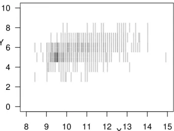
Figure 1: Histogram plot of the red wine data set with n= 1 599 observations. The darker a line segment the more observations overlap this line segment.
of the explanatory variables. This is because, whenV∗
is of the form [X(1), X(1)]×. . .×[X(d), X(d)]
×[Y , Y],
in generalEPˆV∗,λ is no longer convex, and moreover, Theorem 1 does not apply toEPˆV∗,λanymore.
4 SVR Analysis of Wine Quality
In this section, we analyze a data set collected to study the quality of Vinho Verde wines from Portugal. The data were obtained from wine samples that were tested by the official certification entity of the system of protected designation of origin of the Vinho Verde wines between May 2004 and February 2007. For each of the included 1 599 red and 4 898 white wines, 11 physicochemical characteristics and an evaluation of the sensory quality are available. The data set was initially analyzed by Cortez et al. (2009) and is freely available from the UC Irvine Machine Learning Repository (Lichman, 2013). Here, we focus on the subsample of red Vinho Verde wines and study the relationship between taste and alcohol content. In the data set, the sensory quality of the wine is mea-sured on a discrete scale ranging from 0 – very bad to 10 –excellent. These discrete quality measurements should, in fact, be considered as coarse observations of an underlying continuous variable taking values in [0,10]. Therefore, instead of analyzing the discrete values as if they were precise measurements of the wine quality, we consider them to be interval data and replace the discrete values 0,1, . . . ,9,10 by the in-tervals [0,0.5],[0.5,1.5], . . . ,[8.5,9.5],[9.5,10], respec-tively. The alcohol content of the wines is available as volume percent of alcohol, which we here assume to be measured with sufficient precision.8
9
10
11
12
13
14
15
0
2
4
6
8
10
X
Y
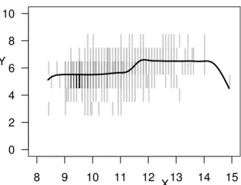
Figure 2: Minimax function of the generalized SVR analysis with linear kernel,ψ(r) =r2for allr∈R≥0,
andλ= 0.0001.
Hence, we analyze the relationship between the pre-cisely observed alcohol content and the imprepre-cisely observed sensory quality of the red Vinho Verde wine. Thus, as we consider only one explanatory variable here, the imprecise data are line segments. The ana-lyzed data set is displayed in Figure 1, whereX is the alcohol level in percent by volume andY corresponds to the sensory quality. All graphs and computations are realized in the statistical software environment R (R Core Team, 2014), resorting amongst others to func-tions provided by the packageskernlab(Karatzoglou et al., 2004) andquadprog(Turlach and Weingessel, 2013).
A red wine lover would probably hypothesize that the higher the alcohol content of a red wine, the stronger and possibly better the taste of the wine. As also the data suggest a positive linear relationship, in the first instance, we choose the linear kernel function for the SVR analysis, although SVR is not limited to linear re-gression. Furthermore, we consider the Least Squares loss, i.e., we setψ(r) =r2for allr∈R≥0. This
config-uration of SVR corresponds to what is also known as Ridge regression. As the minimax approach appears to be more cautious, we consider the corresponding generalized SVR method of Utkin and Coolen (2011) here. Finally, for the estimation, the regularization parameterλis set to 0.0001. The estimated regression line confirms the surmise of a positive relationship between alcohol content and sensory quality of the Vinho Verde red wines and is displayed in Figure 2. As the assumption of a linear relationship is very strict, we alternatively consider the minimax SVR method based on the Gaussian kernel with parameter σequal to 1. Furthermore, we consider the absolute
8
9
10
11
12
13
14
15
0
2
4
6
8
10
X
Y
Figure 3: Minimax function of the generalized SVR analysis with Gaussian kernel,ψ(r) =rfor allr∈R≥0,
andλ= 0.000001.
loss here represented by ψ defined as ψ(r) = r for all r ∈ R≥0 and set λ = 0.000001. The estimated
regression function is depicted in Figure 3 and shows an increasing tendency in those areas of the observation spaceV = [8,15]×[0,10] where most observations are.
Hence, also the more general SVR analysis provides evidence for a positive relationship between alcohol content and sensory quality of red Vinho Verde wines.
5 Conclusion and Outlook
In this paper, we investigated the generalized SVR methods for regression with interval data that were initially proposed by Utkin and Coolen (2011). These methods consist in minimizing either the minimal or the maximal regularized risk compatible with the em-pirical distribution of the imprecise data. In this paper, we proved that the corresponding optimal functions can be represented as the weighted sum of kernel functions and thereby provide the so far lacking justi-fication for the regression methods derived in Utkin and Coolen (2011). Hence, the minimin and minimax SVR methods constitute sensible adaptations of the SVR methodology to interval data and yield interest-ing results when applied to real data as in the previous section.
We here focused on the data situation where only for the response variable there are interval-valued obser-vations, while the explanatory variables are precisely observed. Unfortunately, our findings cannot simply be generalized to account also for interval-valued obser-vations of the explanatory variables, because then the regularized lower risk is no longer necessarily convex and the Representer Theorem cannot be transferred to the regularized upper risk anymore. This means that
for the minimin SVR method there is not necessarily a unique optimal function and that the optimal mini-max function cannot be expanded as in Equation (2). This indeed limits the applicability of the minimin and minimax SVR methods to the more restrictive setting considered in this paper. Moreover, the meaning of the estimated regression functions is less clear than in the precise data case.
Furthermore, it can be argued that, in the context of the statistical analysis of imprecise data, methods yielding precise results are in general problematic, be-cause a reasonable statistical method should reflect the imprecision of the data in its result. In addition, a responsible statistical analysis should always take the involved statistical uncertainty into account. A regression methodology for imprecise data allowing to express these two types of uncertainty at the same time constitutes the so-called Likelihood-based Imprecise Regression (LIR) methodology introduced by Catta-neo and Wiencierz (2012). In the LIR methodology, each possible regression function is evaluated by the whole set of loss values that are plausible in the light of the data and then the set of all undominated re-gression functions is considered as the imprecise result of the regression analysis, which can furthermore be interpreted as a confidence set. As it can be shown that, for eachf ∈ F, the interval [EPˆV∗(f),EPˆV∗(f)] is the Maximum Likelihood estimate ofEPV(f) in the situation considered in Section 3, Utkin and Coolen (2011)’s SVR methods can be further generalized by
embedding them in the LIR framework.
References
Boyd, S., and Vandenberghe, L. (2004).Convex Opti-mization. Cambridge University Press.
Cattaneo, M., and Wiencierz, A. (2012). Likelihood-based Imprecise Regression. International Journal of Approximate Reasoning53, 1137–1154.
Christmann, A., Van Messem, A., and Steinwart, I. (2009). On consistency and robustness properties of
Support Vector Machines for heavy-tailed distribu-tions. Statistics and Its Interface 2, 311–327. Cortez, P., Cerdeira, A., Almeida, F., Matos, T., and
Reis, J. (2009). Modeling wine preferences by data mining from physicochemical properties. Decision Support Systems47, 547–553.
Destercke, S., Dubois, D., and Chojnacki, E. (2008). Unifying practical uncertainty representations: I. Generalized p-boxes. International Journal of Ap-proximate Reasoning49, 649–663.
Ferson, S., Kreinovich, V., Ginzburg, L., Myers, D., and Sentz, K. (2003).Constructing Probability Boxes and Dempster-Shafer Structures. Technical Report SAND2002-4015, Sandia National Laboratories. Hable, R. (2012). Asymptotic normality of support
vector machine variants and other regularized kernel methods. Journal of Multivariate Analysis106, 92– 117.
Hofmann, T., Schölkopf, B., and Smola, A. (2008). Kernel methods in machine learning. The Annals of Statistics36, 1171–1220.
Karatzoglou, A., Smola, A., Hornik, K., and Zeileis, A. (2004). kernlab – An S4 package for kernel methods
in R. Journal of Statistical Software 11, 1–20. Lichman, M. (2013). UCI Machine Learning
Reposi-tory.
R Core Team (2014). R: A Language and Environ-ment for Statistical Computing. R Foundation for Statistical Computing. Used R version 2.15.2. Steinwart, I., and Christmann, A. (2008). Support
Vector Machines. Springer.
Turlach, B., and Weingessel, A. (2013). quadprog: Functions to solve Quadratic Programming Prob-lems. R package version 1.5-5.
Utkin, L., and Coolen, F. (2011). Interval-valued re-gression and classification models in the framework of machine learning. In ISIPTA ’11, Proceedings of the Seventh International Symposium on Impre-cise Probability: Theories and Applications, eds. F. Coolen, G. de Cooman, T. Fetz, and M. Ober-guggenberger. SIPTA, 371–380.
Utkin, L., and Destercke, S. (2009). Computing expec-tations with continuous p-boxes: Univariate case. International Journal of Approximate Reasoning50, 778–798.
Vapnik, V. (1995).The Nature of Statistical Learning Theory. Springer.