VARIABLE SELECTION FOR ULTRA HIGH DIMENSIONAL DATA
A Dissertation by QIFAN SONG
Submitted to the Office of Graduate and Professional Studies of Texas A&M University
in partial fulfillment of the requirements for the degree of DOCTOR OF PHILOSOPHY
Chair of Committee, Faming Liang Committee Members, Raymond Carroll
Valen Johnson Soumendra Lahiri Jianxin Zhou Head of Department, Simon Sheather
August 2014
Major Subject: Statistics
ABSTRACT
Variable selection plays an important role for the high dimensional data analysis. In this work, we first propose a Bayesian variable selection approach for ultra-high dimensional linear regression based on the strategy of split-and-merge. The proposed approach consists of two stages: (i) split the ultra-high dimensional data set into a number of lower dimensional subsets and select relevant variables from each of the subsets, and (ii) aggregate the variables selected from each subset and then select relevant variables from the aggregated data set. Since the proposed approach has an embarrassingly parallel structure, it can be easily implemented in a parallel architecture and applied to big data problems with millions or more of explanatory variables. Under mild conditions, we show that the proposed approach is consistent. That is, asymptotically, the true explanatory variables will be correctly identified by the proposed approach as the sample size becomes large. Extensive comparisons of the proposed approach have been made with the penalized likelihood approaches, such as Lasso, elastic net, SIS and ISIS. The numerical results show that the proposed approach generally outperforms the penalized likelihood approaches. The models selected by the proposed approach tend to be more sparse and closer to the true model.
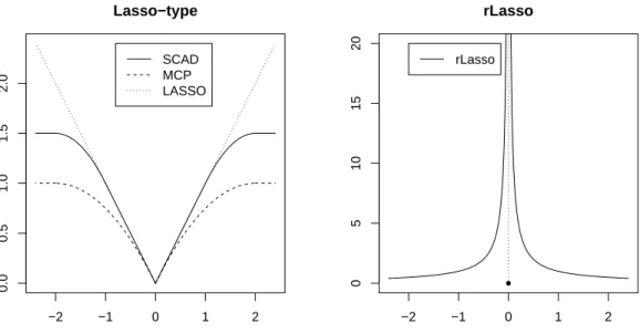
In the frequentist realm, penalized likelihood methods have been widely used in variable selection problems, where the penalty functions are typically symmetric about 0, continuous and nondecreasing in (0,∞). The second contribution of this work is that, we propose a new penalized likelihood method, reciprocal Lasso (or in short, rLasso), based on a new class of penalty functions which are decreasing in (0,∞), discontinuous at 0, and converge to infinity when the coefficients approach
zero. The new penalty functions give nearly zero coefficients infinity penalties; in contrast, the conventional penalty functions give nearly zero coefficients nearly zero penalties (e.g., Lasso and SCAD) or constant penalties (e.g.,L0 penalty). This
distin-guishing feature makes rLasso very attractive for variable selection: It can effectively avoid selecting overly dense models. We establish the consistency of the rLasso for variable selection and coefficient estimation under both the low and high dimensional settings. Since the rLasso penalty functions induce an objective function with mul-tiple local minima, we also propose an efficient Monte Carlo optimization algorithm to solve the minimization problem. Our simulation results show that the rLasso out-performs other popular penalized likelihood methods, such as Lasso, SCAD, MCP, SIS, ISIS and EBIC. It can produce sparser and more accurate coefficient estimates, and have a higher probability to catch true models.
ACKNOWLEDGEMENTS
I would have never been able to finish my dissertation without the guidance of my committee members, help from friends, and support from my family.
Foremost, I would like to express my sincere gratitude to my Ph.D. advisor Prof. Faming Liang for his constant encouragement and support of my Ph.D study and research, for his patience, motivation and passion. His guidance and caring helped me in all the time of my research and writing of this dissertation. I could not have imagined having a better advisor and mentor.
Besides, I would like to thank the rest of my thesis committee: Prof Raymond Carroll, Prof. Valen Johnson, Prof. Soumendra Lahiri and Prof. Jianxin Zhou, for their insightful comments and suggestions. And my special thank goes to Dr. Ellen Toby, for offering my the opportunities to work for her as a teaching assistant.
I would also like to thank many of my fellow postgraduate students in our de-partment: Dr. Yichen Cheng, Dr. Rubin Wei, Dr. Kun Xu, Ranye Sun, Jinsu Kim, Abhra Sarkar, Karl Gregory, Xiaoqing Wu, Nan Zhang, Dr. Yanqing Wang, for their kindness and friendship.
The Department of Statistics and Institute of Applied Mathematics and Compu-tational Science have provided the support and equipment I have needed to produce and complete my thesis.
Last but not the least, I thank my parents and my wife for their unconditional love and support.
TABLE OF CONTENTS
Page
ABSTRACT . . . ii
ACKNOWLEDGEMENTS . . . iv
TABLE OF CONTENTS . . . v
LIST OF FIGURES . . . vii
LIST OF TABLES . . . viii
1. INTRODUCTION: VARIABLE SELECTION AND HIGH DIMENSION-ALITY . . . 1
1.1 History of High Dimensional Variable Selection . . . 1
1.2 Two Proposed Approaches . . . 6
2. BAYESIAN APPROACH: SPLIT AND MERGE STRATEGY AND BIG DATA ANALYSIS . . . 10
2.1 Variable Selection Consistency of the SaM Approach . . . 10
2.1.1 Posterior Consistency for Correctly Specified Models . . . 11
2.1.2 Variable Screening and Selection for Correctly Specified Models 18 2.1.3 Variable Screening for Misspecified Models . . . 26
2.2 SaM Approach and Its Implementation . . . 31
2.2.1 SaM Approach . . . 31
2.2.2 Simulation and Hyperparameter Setting . . . 32
2.3 Simulated Examples . . . 33
2.3.1 Toy Examples . . . 33
2.3.2 Massive Data Example . . . 38
2.4 Real Data Examples . . . 41
2.4.1 mQTL Example . . . 41
2.4.2 PCR Example . . . 44
3. FREQUENTIST APPROACH: RECIPROCAL LASSO PENALTY . . . . 46
3.1 Low Dimensional Regression . . . 46
3.3 Computational Strategy for rLasso . . . 59
3.3.1 Monte Carlo Optimization . . . 59
3.3.2 Tuning Parameter λ . . . 62
3.4 Numerical Studies and Real Data Applications . . . 62
3.4.1 Study I: Independent Predictors . . . 64
3.4.2 Study II: Dependent Predictors . . . 67
3.4.3 Real Data Analysis . . . 71
4. CONCLUSIONS AND DISCUSSIONS . . . 74
REFERENCES . . . 78
APPENDIX A. PROOF OF THEOREMS IN SECTION 2 . . . 87
A.1 Proofs of Theorem 2.1.1 and Theorem 2.1.2 . . . 87
A.2 Proofs of Theorem 2.1.3 and Theorem 2.1.4 . . . 93
A.3 Proof of Theorem 2.1.5 . . . 99
APPENDIX B. PROOF OF THEOREMS IN SECTION 3 . . . 103
B.1 Proof of Theorem 3.1.1 . . . 103
B.2 Proof of Theorem 3.2.1 . . . 105
APPENDIX C. MISCELLANEOUS MATERIAL . . . 114
C.1 Computation Issue of Bayesian Variable Selection . . . 114
LIST OF FIGURES
FIGURE Page
1.1 Distribution of spurious correlation due to dimensionality . . . 2 2.1 Simulation results for marginal inclusion probabilities . . . 35 2.2 Simulation results for MAP model . . . 36 2.3 Simulation results for marginal inclusion probabilities under extremely
high multicollinearity . . . 37 2.4 Results comparison for real mQTL data set . . . 42 2.5 Results comparison for real PCR data set . . . 45 3.1 Discontinuous thresholding functions for three variable selection criteria 48 3.2 Comparison of shapes of different penalty functions. . . 51 3.3 Regularization paths of SCAD, LASSO and rLasso for a simulated
example. . . 53 3.4 Zoomed regularization paths of SCAD, LASSO and rLasso for a
sim-ulated example . . . 54 3.5 Results comparison under independent scenario between rLasso, MCP,
EBIC, Lasso and SIS-SCAD for the datasets simulated in study I . . 65 3.6 Illustration of SAA performance . . . 68 3.7 Results comparison under dependent scenario between rLasso, MCP,
EBIC, Lasso and SIS-SCAD for the datasets simulated in study II . . 69 C.1 Failure of Bayesian shrinkage prior for high dimensional data . . . 116
LIST OF TABLES
TABLE Page
2.1 Simulation results of SaM algorithm for the second toy example . . . 38
2.2 Simulation results for half-million-predictor data sets . . . 39
3.1 Severeness of multicollinearity of the simulated dependent data sets . 70 3.2 Results comparsion for real PCR data set . . . 73
C.1 Failure of Bayesian shrinkage prior for high dimensional data . . . 115
C.2 Full simulation result for rlasso under independent scenario . . . 119
1. INTRODUCTION: VARIABLE SELECTION AND HIGH DIMENSIONALITY
1.1 History of High Dimensional Variable Selection
Variable selection is fundamental to statistical modeling of high dimensional prob-lems which nowadays appear in many areas of scientific discoveries. Consider the linear regression model:
y=Xβ+, (1.1)
where y = (y1, . . . , yn)T ∈ Rn is the response variable, β = (β1, . . . , βp)T ∈ Rp is
the vector of regression coefficients, X = (x1, . . . ,xp)∈ Rn×p is the design matrix,
xi ∈ Rn is the ith predictor, = (1, . . . , n)T ∈ Rn, and i’s are independently
identically distributed (i.i.d.) random variables with mean 0 and varianceσ2. Under
the high dimensional setting, one often assumes that p n and p can increase with n, whilst the true model is sparse, i.e. there are only few predictors whose regression coefficients are nonzero. Such a sparsity assumption is introduced by either a mathematical requirement in order to derive a solution or an expert’s opinion that only few key predictors can causally influence the outcome. Identification of the causal predictors (also known as true predictors) is of particular interest, as which can avoid overfitting in model estimation and yield interpretable systems for future studies.
When analyzing data in the high dimensional spaces, a phenomenon, that we always encounter, is so called the curse of dimensionality. In the problem of model selection, the total number of candidate models is 2p, which increases exponentially
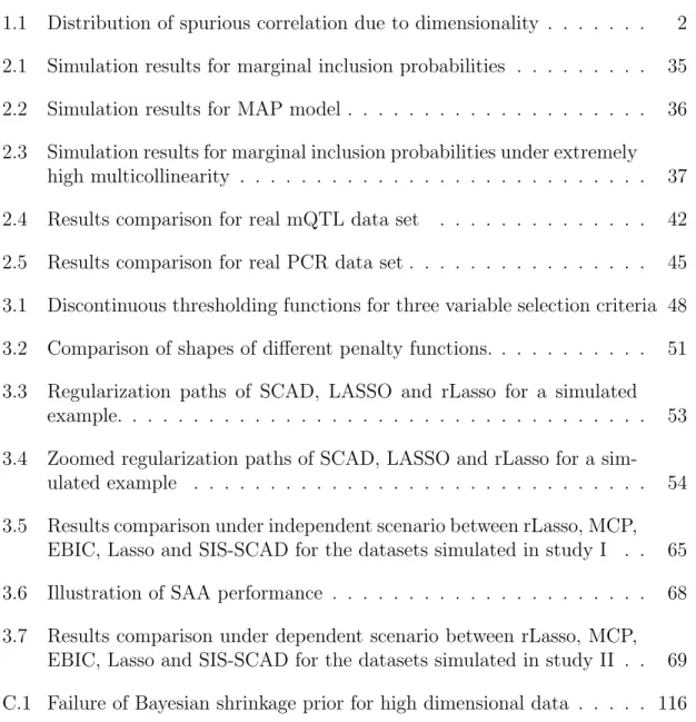
is the noise accumulation. If we have to estimate all p parameters, the accumulated noise by the parameter estimations leads to poor prediction. The second is the spuri-ous correlation. As pointed out by [21], even independent variables will demonstrate very high sample correlation under the high dimensional situation. Figure 1.1 gives the estimated distributions of maximum absolute sample correlation and distribu-tion of the maximum absolute sample correladistribu-tion provided that the variables are generated by independent normal distribution, with n = 50 and p= 1000 or 10000. As a result, any variable, especially the true important one, can be approximated by other spurious variables, and it may lead to a total wrong conclusion.
0.3 0.4 0.5 0.6 0.7
0
5
10
15
Maximum absolute sample correlation
Density p=1000 p=10000 0.70 0.75 0.80 0.85 0.90 0.95 1.00 0 5 10 15 20 25 30 35
Maximum absolute multiple correlation
Density
p=1000 p=10000
Figure 1.1: Distribution of spurious correlation due to dimensionality. Left: distri-bution of maximum absolute sample correlation with n=50; Right: distridistri-bution of the maximum absolute multiple correlation, with n = 50.
In the literature, the problem of variable selection is often treated with penalized likelihood methods. For linear regression, as the dispersion parameter σ can be estimated separately from β, the variable selection can be done by minimizing the
penalized residual sum of squares ˆ β= arg min β {ky−Xβk 2+P λ(β)}, (1.2)
where Pλ(·) is the so-called penalty function and λ is a tuning parameter which
can be determined via cross-validation. The penalty function serves to control the complexity of the model, and its choice determines the behavior of the method. [65] proposed the Lasso method which employs a L1-penalty of the form
Pλ(β) =λ p
X
i=1
|βj|.
Since Lasso gives small penalties to small coefficients , the resulting model tends to be dense, which may include many spurious predictors with very small coefficients. As shown in [71] and [72], Lasso might not be consistent for variable selection unless a strong representable condition holds. To remedy this flaw, various methods have been proposed, such as adaptive Lasso [72], SCAD [18], and MCP [69]. Adaptive Lasso assigns different weights for penalizing different coefficients in theL1 penalty. SCAD
and MCP employ some penalty functions that are concave on (0,∞) and converge to constants as |β|becomes large, and thus reduce the estimation bias when the true coefficients are large. Although these methods have shown some improvements over Lasso, they still tend to produce dense models especially when the ratio log(p)/n is large. This is because, as illustrated in Section 3, these methods share the same feature with the Lasso that nearly zero coefficients are given nearly zero penalties.
[11] showed that subject to theL1 penalty, the estimator ofβ can only achieve a
mean squared error up to a logarithmic factor log(p). Motivated by this result, [19] and [20] proposed the sure independence screening (SIS) method and its iterative
version, iterative SIS (ISIS). The SIS is to first reduce the dimension pby screening out the predictors whose marginal utility is low, and then apply a penalized likelihood method, such as Lasso or SCAD, to select appropriate predictors. The marginal utility measures the usefulness of a single predictor for predicting the response, and it can be chosen as the marginal likelihood or simply the marginal correlation for linear regression. ISIS iteratively selects predictors from remaining unselected predictors and thus reduces the risk of missing true predictors. Since many false predictors can be removed in the screening stage, SIS and ISIS can generally improve the performance of Lasso and SCAD in variable selection.
Back to 1970’s, [1, 2] proposed the AIC which is to select predictors by minimizing the Kullback-Leibler divergence between the fitted and true models. Later, [60] proposed the Bayesian information criterion (BIC). Both AIC and BIC employ the L0 penalty, which is given by
Pλ(β) = p
X
i=1
λI(βi 6= 0).
Recently, BIC has been extended to high dimensional problems by [12, 13], which establish the consistency of the extended BIC (EBIC) method for variable selection under the conditionsp=O(nκ) andλ= log(n)/2 +γlog(p), whereγ >1−1/2κis a
user-specified parameter. TheL0-regularization method has a natural interpretation
of best subset selection, where each coefficient is penalized by a constant factor. It is easy to figure out that this constant factor is of order O(log(p)). Compared to the Lasso-type penalties, such as those used in Lasso, adaptive Lasso, SCAD and MCP, the L0-penalty overcomes the drawback of small coefficients small penalties.
However, for the problems for which the ratio log(p)/n is large, a penalty of order O(log(p)) seems too big. It is known that the models produced by EBIC under
this scenario tend to be overly sparse. Other major concern with EBIC is the lack of an efficient optimization algorithm to search over the model space. Because the model space is discrete, some computationally intensive algorithms, such as Markov chain Monte Carlo (MCMC), have to be used. We note that the SCAD and MCP penalties can also be viewed as an approximation to theL0 penalty, as they converge
to constants when the coefficients become large.
Parallel to the penalized likelihood approaches, various Bayesian approaches have also been developed to tackle this problem. These approaches advance either in a sophisticated model search algorithm, such as evolutionary stochastic search [8], or in a prior specification that is particularly suitable for high dimensional problems, such as the Lasso prior [56], Ising prior [47], proportion of variance explanation (PVE) prior [29], and nonlocal prior ([37], [36]). Although various numerical examples have demonstrated the successes of Bayesian approaches on this problem, there still lacks a rigorous theory to show that the Bayesian approaches can lead to a consistent selection of true predictors when p is greater than n. On the other hand, the high computational demand of Bayesian approaches for sampling from the posterior dis-tribution also hinders their popularity. Since the volume of the model space increases geometrically with the dimension p, the CPU time for a Bayesian approach should increase accordingly or even faster.
It is interesting to point out that many Bayesian variable selection methods are closely related to the L0 penalty, see e.g., g-prior ([68], [51]), evolutionary stochastic
search [8], and Bayesian subset selection (BSR) [52]. In these methods, a hierarchical prior is assumed for the model size and the regression coefficients associated with the model. For example, a commonly used prior for the model size is
whereξ denotes the selected model with size|ξ|, and µdenotes the prior probability that each predictor can be included in the model. The hyperparameter µ can be either determined using the empirical Bayes method [25] or treated as a beta random variable in a fully Bayesian method. It follows from [61] that both choices of µwill result in a prior of model size that is approximately equivalent to the L0 penalty.
Under the high dimensional setting,µcan also be chosen as a decreasing function ofp as suggested by [52]. Like the empirical and fully Bayesian methods, this choice ofµ also induces an automatic multiplicity adjustment for variable selection. It is worth pointing out that under the prior specification of [52], the maximum a posteriori (MAP) model is reduced to the EBIC model.
1.2 Two Proposed Approaches
In this work, two new approaches are proposed to solve the high dimensional vari-able selection problems in both Bayesian and Frequentist frameworks. The proposed Bayesian variable selection approach based on the strategy of split-and-merge. The proposed approach consists of two stages:
(i) Split the high dimensional data into a number of lower dimensional subsets and perform Bayesian variable selection for each subset.
(ii) Aggregate the variables selected from each subset and perform Bayesian vari-able selection for the aggregated data set.
Under mild conditions, we show that the proposed approach is consistent. That is, the true model will be identified in probability 1 as the sample size becomes large. Henceforth, we will call the proposed approach the split-and-merge (SaM) approach for the purpose of description simplicity.
Our contribution in this Bayesian variable selection method is two-fold. First, we propose a computationally feasible Bayesian approach for ultra-high dimensional
regression. Since SaM has an embarrassingly parallel structure, it can be easily implemented in a parallel architecture and applied to the big data problems with millions or more of predictors. This has been beyond the ability of conventional Bayesian approaches, as they directly work on the full data set. Second, under mild conditions we show that the Bayesian approach can share the same asymptotics, such as sure screening and the model selection consistency, as the SIS approach. In spirit, SaM is similar to SIS. The first stage serves the purpose of dimension re-duction, which screens out uncorrelated predictors; and the second stage refines the selection of predictors. However, compared to SIS and ISIS, SaM can often lead to more accurate selection of true predictors. This is because SaM screens uncorrelated predictors based on the marginal inclusion probability, which has incorporated the joint information of all predictors contained in a subset. While, as previously men-tioned, SIS makes use of only the marginal information of each predictor. ISIS tries to incorporate information from other predictors, but in an indirect way.
Finally, we note that the strategy of split-and-merge, or otherwise known as divide-and-conquer, has been often used in big data analysis, see e.g., [55], [41], [54] and [67]. Our use of this strategy is different from others. In SaM, the data split is done in the dimension of predictors, while this is done in the dimension of observations in other work. This difference necessitates the development of new theory for variable selection under the situation that the model is misspecified due to the missing of some true predictors.
In the second approach, we propose a new class of penalty functions for penalized likelihood variable selection, which are decreasing in (0,∞), discontinuous at 0, and converge to infinity when the coefficients approach zero. The new penalty function
has a typical form of Pλ(β) = p X i=1 λ |βi| I(βi 6= 0),
which gives nearly zero coefficients infinity penalties. In contrast, the conventional penalty functions give nearly zero coefficients nearly zero penalties (e.g., the Lasso-type penalties) or constant penalties (e.g., the L0 penalty). Although unusual, the
new penalty function possesses a very intuitive and appealing interpretation: The smaller coefficient a predictor has, the more likely the predictor is a false predictor and thus the higher penalty it should have. If a predictor has a nearly zero coefficient, then the effect of the predictor on model estimation and future prediction should be very limited and, hence, it had better be excluded from the model for the sake of model simplicity. Our numerical results show that the new penalty can outperform both the Lasso-type penalties and the L0 penalty in identifying true models.
The contribution of this frequentist method is three-fold:
(i) We propose a novel penalty function for variable selection, which overcomes some drawbacks of the existing penalty functions. Compared to the Lasso-type penalties, it gives small coefficients large penalties and thus avoids to select overly dense models. Compared to the L0-penalty, it is coefficient dependent
and thus adaptive for different coefficients; in addition, as discussed at the end of Section 3, it allows the tuning parameter λ to take values at a lower order of log(p) and thus avoids to select overly sparse models.
(ii) We establish the consistency of the new method for variable selection and parameter estimation. Under the low dimensional setting, where p is fixed as n increases, we show that the new method possesses the oracle property. That is, the true model can be consistently selected and the coefficient estimator is as efficient as the ordinary least square (OLS) estimator. Under the high
dimensional setting, where p n and p increases with n, we show that the true model can also be consistently selected, and that the coefficient estimator can converge inL2 and is thus consistent.
(iii) We propose an efficient Monte Carlo optimization algorithm based on the co-ordinate descent ([9], [24]), stochastic approximation Monte Carlo [50] and stochastic approximation annealing [49] algorithms to solve the optimization (1.2) with the proposed penalty function. The proposed optimization algorithm can deal with problems with multiple local minima and is thus also applicable for other L0-regularization methods.
The remaining part of this dissertation is organized as follows. We describe the Bayesian variable selection approach in Section 2. Section 2.1 establishes consis-tency of the SaM approach for variable selection. Section 2.2 summarizes the SaM approach and discusses some implementation issues. Section 2.3 illustrates the per-formance of the SaM approach using two simulated examples along with comparisons with penalized likelihood approaches. Section 2.4 compares the SaM approach with penalized likelihood approaches on two real data examples. In Section 3, we describe our penalized likelihood methods with the new proposed penalty function. In Sec-tion 3.1, we establish the consistency of the new method for variable selecSec-tion and parameter estimation under the low dimensional setting. In Section 3.2, we extend the low dimensional results to the high dimensional case. In Section 3.3, we describe the Monte Carlo optimization algorithm. In Section 3.4, we present some numerical results to illustrate the performance of the new method. In Section 4, we conclude the SaM algorithm and rLasso method with a brief discussion, We present related proofs of the theorems in Section 2 and Section 3 in the Appendix A and Appendix B respectively, and provide some related miscellaneous material in Appendix C.
2. BAYESIAN APPROACH: SPLIT AND MERGE STRATEGY AND BIG DATA ANALYSIS
In this section, we address the proposed Split and Merge method for high dimen-sional regression analysis, especially when dealing with massive data set. Before de-scribe the detailed algorithm, we first lay the theoretical background of the Bayesian variable selection consistency in Section 2.1.
2.1 Variable Selection Consistency of the SaM Approach
This section is organized as follows. In Section 2.1.1, we establish the posterior consistency for correctly specified models; that is, if the model is correctly specified with all true predictors included in the set of candidate predictors, the true density of the model (1.1) can be estimated consistently by the density of the models sampled from the posterior as the sample size becomes large. In Section 2.1.2, we establish the sure screening property for the correctly specified models based on the marginal inclusion probability; that is, the marginal inclusion probability of the true predictors will converge to 1 in probability as the sample size becomes large. In this section, we also establish the consistency of the maximuma posteriori(MAP) model; that is, the MAP model is a consistent estimator of the true model. In Section 2.1.3, we show that for the misspecified models for which some true predictors are missed in the set of candidate predictors, the sure screening property based on the marginal inclusion probability still holds. Combining the theoretical results established in Sections 2.1.1 to Section 2.1.3 leads to the variable selection consistency of the SaM approach.
2.1.1 Posterior Consistency for Correctly Specified Models
LetDn={y;x1, . . . ,xpn}denote a data set ofn observations drawn from model (1.1). Let x= (x1, . . . , xpn)
T denote a generic observation of the p
n predictors, and
let y denote a generic observation of the response variable corresponding to x. Let νx denote the probability measure of x. Then the true probability density of (y, x)
is given by f∗(y, x)dxdy= √ 1 2πσ∗ exp −(y−x Tβ∗ )2 2σ∗2
νx(dx)dy=φ(y;xTβ∗, σ∗)νx(dx)dy,
(2.1) where φ(·;µ, σ) denotes a Gaussian density function with mean µand standard de-viation σ.
As in conventional studies of high dimensional variable selection, we consider the asymptotics of the SaM approach under the assumption that pn increases as n
increases. To be specific, we assume that pn nθ for some θ > 0, where bn an
means limn→∞an/bn= 0. In addition, we assume that the true model is sparse. Two
sparseness conditions are considered in this work. One states that most components of β∗ are very small in magnitude such that
lim n→∞ pn X j=1 |βj∗|<∞, (2.2)
where βj∗ denotes the jth entry of β∗. The other one is stronger but more usual, which requires that most components of β∗ are zero such that
lim n→∞ pn X j=1 1{βj∗ 6= 0}<∞. (2.3)
selected predictors. Let |ξ| denote the number of predictors included in ξ. Thus, the strict sparsity condition (2.3) implies that the true model t = {i : βi∗ 6= 0,1 ≤ i ≤ pn} has a finite model size. For a model ξ = {i1, i2, . . . , i|ξ|}, we let Xξ =
(xi1,xi2, . . . ,xi|ξ|) denote the design matrix, and let βξ = (βi1, . . . , βi|ξ|)
T denote the
regression coefficient vector. Let L(Dn|ξ,βξ, σ2) denote the likelihood function, and
letπ(ξ, dβξ, dσ2) denote the joint prior distribution imposed onξand the parameters σ2 and βξ. Then the posterior distribution is given by
π(ξ, dβξ, dσ2|Dn) = L(Dn|ξ,βξ, σ2)π(ξ, dβξ, dσ2) P ξ R βξ,σ2L(Dn|ξ,βξ, σ 2)π(ξ, dβ ξ, dσ2) . (2.4) 2.1.1.1 Prior Specification
For the modelξ, we assume that each predictor has a prior probabilityλn =rn/pn,
independent of other predictors, to be included in the model ξ. Further, we impose a constraint on the model size such that|ξ| ≤¯rn, where the model size upper bound
¯
rn is pre-specified. Then we have
π(ξ)∝λ|ξ|n (1−λn)pn−|ξ|I[|ξ| ≤r¯n]. (2.5)
The constraint on |ξ| is not crucial to the data analysis. Since the true model is sparse, there is not much loss as long as the size of the true model is less than ¯
rn. From the perspective of computation, such a constraint facilitates the posterior
simulation, as the computational complexity of the likelihood evaluation is O(|ξ|3),
which involves inverting a covariance matrix of size |ξ| by |ξ|.
We let the variance σ2 be subject to an Inverse-Gamma prior distribution with the hyper-parameters a0 and b0; i.e., σ2 ∼ IG(a0, b0). Conditioned on the model ξ
and σ2, we let β
ξ be subject to a Gaussian prior,
βξ|ξ, σ2 ∼N
|ξ|(0, σ2Vξ),
where Vξ is a positive definite matrix depending onξ.
To facilitate computation, we integrate out βξ and σ2 from the posterior
distri-bution (2.4). The resulting posterior of ξ is given by
π(ξ|Dn)∝(rn/pn)|ξ|(1−rn/pn)pn−|ξ| q det(Vξ−1) q det(XTξXξ+Vξ−1) × 2b0+yT(I−Xξ(XTξXξ+Vξ−1) −1 XTξ)y −n/2−a0I[|ξ| ≤r¯n]. (2.6)
For a fully Bayesian variable selection approach, λn is usually subject to a Beta
prior. As pointed out by [61], placing such a prior on λn will induce an automatic
multiplicity adjustment for variable selection: The penalty for adding an extra vari-able increases aspnincreases. The multiplicity control is crucial for variable selection
when pn is greater than n. Otherwise, the resulting model tends to be liberal. For
example, the BIC criterion places a flat prior for the model ξ, and the resulting models are overly liberal for high dimensional regression [10]. In this work, we as-sume λn → 0 as pn → ∞, which corresponds to condition (2.12) in Theorem 2.1.1.
This condition provides an automatic mechanism of multiplicity control for the SaM approach.
The posterior (2.6) is also closely related to the EBIC criterion [12], which is to choose a model ξ by minimizing the penalized likelihood function
EBIC(ξ) =−ˆl(ξ) + |ξ|
where ˆl(ξ) is the loglikelihood function of ξ evaluated at the maximum likelihood estimates of βξ and σ2. If we set V−1
ξ =X T ξXξ/n, a0 =b0 ≈0, andrn =p1−γn for a constantγ ∈(0,1), thenXTξXξ+Vξ−1 ≈X T ξXξ and log(rn/pn)|ξ|(1−rn/pn)pn−|ξ|≈
−γ|ξ|logpn+p1−γn . Therefore, logπ(ξ|Dn) ≈ −EBIC(ξ) +C for some constant C
independent of ξ. A similar approximation between the posterior and EBIC can be found in [52] for generalized linear models.
2.1.1.2 Posterior Consistency
In what follows, we study the asymptotics of the posterior distribution with respect to the Hellinger distance under appropriate conditions of rn, ¯rn and Vξ. For
two density functions f1(x, y) and f2(x, y), the Hellinger distance is defined as
d(f1, f2) =
s
Z Z
(f11/2(x, y)−f21/2(x, y))2dxdy.
For a matrix Σ, we let chi(Σ) denote the ith largest eigenvalue, and let ch0i(Σ)
denote the ith smallest eigenvalue. Define B(rn) = supξ:|ξ|=rnch1(V
−1
ξ ), ¯B(rn) =
supξ:|ξ|=rnch1(Vξ), ˜Bn= supξ:|ξ|≤¯rnch1(Vξ), and ∆(p) = infξ:|ξ|=p
P
i /∈ξ|β ∗ i|.
Theorem 2.1.1 follows from [35]. Here we consider one of the simplest situations that all predictors have been standardized and uniformly bounded, and the sparsity condition (2.2) holds.
Theorem 2.1.1 (Posterior Consistency). Assume that the data setDnis drawn from
that n2
n1, and the following conditions hold:
∆(rn)≺n, (2.7) ¯ rnln(1/2n)≺n 2 n, (2.8) ¯ rnln(pn)≺n2n, (2.9) ¯ rnln(n2nB˜n)≺n2n, (2.10) 1≤rn≤r¯n< pn, (2.11) rn≺pn, (2.12) B(rn)≺n2n, (2.13)
then the posterior consistency holds, i.e., there exists a constant c1 >0 such that
P∗{π[d(f, f∗)> n|Dn]> e−c1n
2
n}< e−c1n2n, (2.14)
for sufficiently large n, where the Hellinger distance is
d2(f, f∗) =
Z Z
|φ1/2(y;xTβ∗
, σ∗)−φ1/2(y;xTβ, σ)|2ν
x(dx)dy,
where f∗ is as defined in (2.1), f is the density function for a model simulated from the posterior, and P∗ denotes the probability measure of data generation.
The proof of Theorem 2.1.1 can be found in the Appendix. The validity of this theorem depends on the choice of the prior covariance matrix Vξ, or more precisely,
the largest eigenvalues of Vξ and Vξ−1. For most choices of Vξ, B(rn) ≤ Brvn and
˜
Bn ≤ Brvn hold for some positive constants B and v. For example, if Vξ = cI|ξ|,
where Ip is an identity matrix of order p, then both B(rn) and ˜Bn are constants.
replaced by its sample empirical estimator. If all xi’s are standardized with zero
mean and equal variance, then B(rn) ≤ rn. Furthermore, if xi has some specific
covariance structure, then ˜Bn can be shown to be bounded. For example, if all
pairwise covariance cov(xi, xj) = ρ ∈ (0,1), then ˜Bn = 1 −ρ; if xi is generated
from a finite order autoregressive (AR) or moving average (MA) model without root for the characteristic polynomial on the unit circle, then ˜Bn is also bounded by
some constant [7]. In general, for standardizedxi’s, we can choose a “ridge prior” as
suggested by [31]: LetVξ−1 =E(xTξxξ) +cnI|ξ|, thenB(rn)≤rn+cnand ˜B(n)≤c−1n ,
where cn is proportional to 1/n, i.e., cn ∝n−1.
Theorem 2.1.1 assumes that all the predictors are uniformly bounded. However, this condition might not be satisfied for continuous predictors. In what follows, we relax this condition:
(A1) There exist some constants M >0 andδ >0 such that for any subvector of x,
(xj1, ..., xjr) T with 1≤j 1 <· · ·< jr ≤pn, r ≤r¯n, and |ai| ≤δ for i= 1, . . . , r, we have Eexp r X i=1 aixji/r !2 ≤exp(M),
where the expectation is taken with respect to the distribution of the random vari-ables xji’s.
The condition (A1) controls the tail distribution of x such that the marginal
dis-tribution of y does not change dramatically in the sense of d1 divergence (defined in
the Appendix) with respect to the change of β. If x has a heavy tail distribution, the prior information around f∗ will be too weak to induce good posterior asymp-totics. If all the variables are bounded by some constant m, as assumed in Theorem 2.1.1, then Eexpn(Pr
i=1aixji/r)
2o
≤ exp(δ2m) and thus (A1) holds. If x follows a
Gaussian process with zero mean and Var(xi) = 1, then (Pri=1aixji)
2 follows thesχ2 1
distribution, where the scales ≤δ2r2. Therefore, by the moment generating function of χ2 1 distribution, Eexp n (Pr i=1aixji) 2 /r2o≤(1−2δ2)−1/2, condition (A 1) holds.
Under the condition (A1), we have the following theorem whose proof can be
found in the Appendix.
Theorem 2.1.2. Assume that the data set Dn is generated from model (1.1) and all
the predictors satisfy condition (A1). Given a sequence {n}, n→0, and n2n → ∞.
If the conditions (2.8) to (2.13) of Theorem 2.1.1 hold, the model is strictly sparse, i.e. condition (2.3) holds, and rn1, then the posterior consistency still holds, i.e.,
there exists a constant c1 >0 such that for sufficiently large n,
P∗{π[d(f, f∗)> n|Dn]> e−c1n
2
n}< e−c1n2n.
Note that condition (2.7) of Theorem 2.1.1 is redundant here, as for large n, rn >|t|and ∆(rn) = 0 hold under the sparseness condition (2.3). The next corollary
concerns the convergence rate of the posterior distribution.
Corollary 2.1.1. Consider a strict sparse model, i.e. condition (2.3) holds. Suppose
that pn < eCn
α
for some α ∈ (0,1), and the prior specification in section 2.1.1.1 is used such that B(rn) ≤ Brnv and B˜n ≤ Bnv for some positive constants B and v.
Take
rn <¯rn ≺logk(n), or rn<r¯n≺nq,
for some k > 0 or some 0 < q < min{1−α,1/v}. Then the convergence rate in Theorem 2.1.2 can be taken as
n=O(n−(1−α)/2logk/2n), or n =O(n−(min{1−α−q,1−vq})/2).
The conditionA1 imposes a stringent requirement for the distribution of the
pre-dictors, although in real world, one may treat any predictor as bounded in practice. If any of the predictor is not heavy tailed distributed, condition A1 fails. A much
weaker condition is proposed in below:
(A2) There exist some constants M >0 andδ >0 such that for any subvector of x,
(xj1, ..., xjr) T with 1≤j 1 <· · ·< jr ≤pn, r ≤r¯n, and |ai| ≤δ for i= 1, . . . , r, we have E r X i=1 aixji/r !2 ≤M.
(A2) only imposes condition on the second moment structure of the predictors, and
if all predictors have uniformly bounded second moment, condition (A2) holds. It
can be showed (in the Appendix), if condition (A2) holds instead of (A1), a slightly
weaker result of theorem 2.1.2 can be still obtained as below,
lim n→∞P ∗{π[d(f, f∗ )> n|Dn]> e−c1n 2 n}= 0. (2.15)
In the appendix, it is showed that under condition (A1),π[d(f, f∗)> n|Dn] converges
in L1 exponentially, while (2.15) only impliesconvergence in probability.
2.1.2 Variable Screening and Selection for Correctly Specified Models
To serve the purpose of variable selection for the case that the true model t exists, i.e. condition (2.3) holds, we need a consistent variable selection procedure. In this section, we consider two procedures, which are based on the marginal inclusion probability and maximum a posteriori(MAP) model, respectively.
2.1.2.1 Marginal Inclusion Probability
Variable selection by marginal inclusion probability has been used in high dimen-sional Bayesian analysis, see e.g., [5] and [52]. In this section, we study the property of marginal inclusion probability based on the posterior convergence result (2.14) or (2.15), which implies that π[d(f, f∗)> n|Dn]
p
→0. Since our objective is to recover all the true predictors, we need to explore the relationship between the distance in distributions and the difference in models. Let qj denote the marginal inclusion
probability of the predictor xj, which is given by
qj =π(j ∈ξ|Dn) =
X
ξ∈{ξ:j∈˜ ξ}˜
π(ξ|Dn).
Intuitively, we expect that a true predictor xt (t ∈ t) will have a high marginal
inclusion probability. However, under high dimensional scenario, spurious multi-collinearity is quite common phenomenon. [66] studied the relationship between low-rankness of design matrix and consistency of the pairwise model Bayes factors and global posterior probabilities given null model is true. If a true predictor can be well-approximated or even replaced by a couple of spurious predictors, hence inclusion probabilities of spurious predictors are inflated. Therefore, in order to consistently select the true variables, it is necessary to control the severeness of mul-ticollinearity. To study the asymptotics of the marginal inclusion probability, we introduce the following identifiability condition:
(B1) A predictor xk is said to be identifiable among all other predictors, if, for any
1≤j1, . . . , j¯rn ≤pn (ji 6=k for all i) and bi ∈R,
Eexp ( −(xk+ ¯ rn X i=1 bixji) 2 ) ≤1−δn, and δn 2n,
where xl denotes a generic observation of the predictor xl.
This condition states that if a predictor xk is identifiable, then there does not exist
a linear combination of other predictors in X which can mimic it. The severeness of collinearity among predictors is controlled by sequence n, and xk can be
distin-guished from other predictors in X.
If all the predictors have mean 0 and are bounded with |xi| ≤1, then
Eexp ( −(xk+ ¯ rn X i=1 bixji) 2 ) ≤E 1− 1−exp{−(1 + P i|bi|) 2} (1 +P i|bi|)2 (xk+ X i bixji) 2 ! ≤1−(1−e−1)Var(xk+ P ibixji) (1 +P|b i|)2 ≤1− 1−e −1 (¯rn+ 1) ch01(Var(˜x)), where ˜x = (xk, xj1, . . . , xjrn¯ ) T, and ch0
1(Var(˜x)) is the smallest eigenvalue of the
covariance matrix of ˜x. Hence, if ch01(Var(˜x)) r¯n2n for any choice of ˜x, xt is
iden-tifiable. Furthermore, if ch01(Var(x)) ¯rn2n, then all the predictors are identifiable,
here x= (x1, . . . , xpn)
T denotes a generic observation of all predictors.
If all the predictors follow the standard normal distribution, by the moment generating function of the chi-square distribution, we have
Eexp{−(xk+ X bixji) 2}= (1 + 2Var(x k+ X i bixji)) −1/2 <max{0.5,1−Var(xk+ X i bixji))/8}. Thus, if Var(xk+ P ibixji) 2
n, then the identifiability condition is satisfied. Since
Var(xk+ X i bixji)≥Var(xk|˜x\xk)≥ch 0 1(Var(˜x))≥ch 0 1(Var(x)),
by the same arguments, all predictors are identifiable ifch01(Var(x))2
n. Further, it
can be shown (in the proof of Theorem 2.1.3) that if a true predictorxtis identifiable,
then d(f∗, f)≥n for any density f that does not select xt. Therefore, we have the
following sure screening property.
Theorem 2.1.3 (Sure Screening). Assume that all the conditions of Theorem 2.1.2
hold. If a true predictor xt (t ∈ t) is identifiable, then P∗{π[t ∈ ξ|Dn] < 1 −
e−c1n2n}< e−c1n2n, where ξ denotes a model sampled from the posterior distribution. Furthermore if condition (A2) holds instead of (A1), then weaker convergence holds:
limnP∗{π[t ∈ξ|Dn]<1−e−c1n
2
n}= 0.
The proof of Theorem 2.1.3 can be found in the Appendix. Letξq ={i: 1≤i≤
pn, qi > q} denote a model including all the predictors with the marginal inclusion
probability greater than a threshold value ofq∈(0,1). Then it follows from Theorem 2.1.3 that π(t ⊂ ξq)
p
→ 1 if all true predictors are identifiable. To determine the threshold value q, we adopt the multiple hypothesis testing procedure proposed in [52], where the procedure is used for selecting variables for a logistic regression model. The procedure can be briefly described as follows.
Let zi = Φ−1(qi) denote the marginal inclusion score (MIS) of the predictor xi,
where Φ(·) is the CDF of the standard normal distribution. To select predictors with large MISs, we model the MISs by a two-component mixture exponential power distribution by
where ϑ = (ω, µ1, µ2, σ1, σ2, α1, α2)T is the vector of parameters of the distribution, and ϕ(z|µi, σi, αi) = αi 2σiΓ(1/αi) exp{ −(|z−µi|/σi)αi}, − ∞< µ1 < µ2 <∞, σi >0, αi >1, (2.17)
where µi, σi, αi are the location parameter, dispersion parameter and decay rate of
the distribution, respectively. If α = 2, then the exponential power distribution is reduced to a normal distribution.
The parameters of (2.16) can be estimated as in [53] by minimizing KL(ϑ) us-ing the stochastic approximation algorithm, where KL(ϑ) is the Kullback-Leibler divergence between g(z|ϑ) and the unknown true distribution g(z):
KL(ϑ) =−
Z
log(g(z|ϑ)/g(z))g(z)dz.
For a given selection rule Λ = {Zi > z0}, the false discovery rate (FDR) of true
predictors can be estimated by
F DR(Λ) = pnω[1−F(z0|µˆ1,σˆ1,αˆ1)] #{zi :zi > z0}
,
whereF(·) denote the CDF of the distribution (2.17), and #{·}denotes the number of elements in a set. Similar to [64], we define the q-value as
Q(z) = inf
{λ:z∈Λ}F DR(Λ). (2.18)
Then a cutoff value of z0, which corresponds to the marginal inclusion probability
α= 0.01 and 0.05. That is, all the predictors belonging to the set{xi :Q(Φ−1(qi))≤
α} will be selected as “true” predictors.
Compared to other FDR control procedures, one advantage of this procedure is that it is applicable under general dependence between marginal inclusion proba-bilities. Refer to [53] for the details of the procedure and its generalization to the m-component case.
2.1.2.2 MAP model
Many Bayesian studies suggest that the MAP model is potentially a good es-timator of the true model, see e.g., [23] and [30]. In what follows, we establish the consistency of the MAP model with two different choices of Vξ: Vξ−1 = I and
Vξ−1 =XTξXξ/n.
Theorem 2.1.4. (Consistency of the MAP model) Let Dn be a data set generated
from model (1.1) with a sparse true model t. Assume condition (2.11) and the following eigen-structure conditions hold: For any model ζ with size |ζ|= min{|t|+ ¯
rn, n}, there exist a non-increasing sequence{ln} and a non-decreasing sequence{ln0}
such that nln< ch01(X T ζXζ)≤ch1(XζTXζ)< nl0n, (2.19) ¯ rnlogpn≺nln. (2.20)
If, further, one of the following two condition holds:
1. nlnlogl0n, log √
nln
rn √
logpn, and we set Vξ−1 =I for any ξ; or
2. nlnln0, log √
n rn
√
logpn, and we set Vξ−1 =X T
then, for any model k, the posterior probability (2.6) satisfies: max k6=t π(k|Dn) π(t|Dn) p →0. (2.21)
This theorem implies that the true model t can be identified asymptotically by just finding out the MAP model under (2.6). Regarding the eigen structure condition (2.19) and the choice of Vξ, we have the following remarks:
• It is worth noting that the eigenvalue condition (2.19) is hardly satisfied, al-though similar conditions have been used in the literature, see e.g., [37]. A feasible condition can be as follows: There exist two sequences {ln} and {ln0}
and a constant C such that for any model |ζ|= ¯rn+|t|,
P rnln> ch01(X T
ζXζ) or ch1(XTζXζ)> nl0n < e −nC
. (2.22)
Since the condition ¯rnlnpn≺n holds, (2.22) implies that, for sufficiently large
n,
P r∃ |ζ|= ¯rn+|t|, nl > ch01(X T
ζXζ) or ch1(XζTXζ)> nl0 < e−nC/2.
Hence, if (2.19) is replaced by (2.22), Theorem 2.1.4 still holds. The condition (2.22) does not require the eigenvalues of the sample covariance matrix to be bounded, but restricts the tail distribution of eigenvalues. Hence, it is more reasonable and acceptable.
• The condition (2.22) is similar to but somewhat weaker than the concentra-tion condiconcentra-tion used in [19]. The concentraconcentra-tion condiconcentra-tion constrains the eigen-structure of anyn×p˜sub-datamatrix for any ˜p > cnfor some constantc, while
the condition (2.22) only constrains the eigen-structure of n×(¯rn+|t|)
sub-datamatrix. In particular, condition (2.22) holds when x follows a Gaussian process, and the eigenvalues of Var(x) are bounded byln and l0n (see Appendix
A.7 of [19]). For a further study of the limit behavior of the spectral structure, see e.g. [63], [4], and [46].
• Choosing Vξ−1 as a function of the sample covariance matrix makes use of the data information in the prior, and as a result, a slightly weaker condition is required for the consistency of variable selection. It follows from the theory of least square regression, a natural choice of Vξ−1 isVξ−1 =XTξXξ/n. However,
for binary data, even if n > |ξ|, one may still encounter the problem of singu-larity of XTξXξ. To address this issue, we set Vξ−1 = (X
T
ξXξ+τ I)/n for some
small τ in our simulations. It can be shown that this choice leads to the same consistency result as with the sample covariance matrix (see Lemma A.2 of the Appendix). This choice also automatically meets the eigenvalue condition of Vξ in Corollary 2.1.1 for a standardized dataset.
Corollary 2.1.2. Consider a linear regression with a sparse true model t. Assume
that pn< nκlogn for some κ ∈(0,1/4), and the prior in Section 2.1.1.1 is used with
Vξ−1 =XTξXξ/n or Vξ−1 =XTξXξ/n+τ I/n. Let ¯ rn ≺logk1(n), or r¯n≺nq, for some k1 >0 or q≤1/2− √ κ, and l0n=l−1n =√n/logk2(n),
Theorem 2.1.3 and Theorem 2.1.4 provide two strategies for variable selection, either by marginal inclusion probability or by the MAP model. Theorem 2.1.4 states that the MAP model is consistent, while Theorem 2.1.3 states only the sure screening property (sensitivity is asymptotically 1, but specificity is not controlled). In this work, we suggest to use marginal inclusion probability as the criterion of variable selection. Under this criterion, one may select more predictors, which are worthy of further investigation through a possibly different and expensive experiment. Since the sample sizen can be small for a real problem, the MAP model might not capture all true predictors although it is consistent in theory.
2.1.3 Variable Screening for Misspecified Models
LetDns={y,Xs}denote a fixed subset of observations, wheres⊂ {1,2, . . . , pn}
and Xs contains only s = |s| < pn predictors with the indices belonging to s.
Assume thatXsdoes not include all of the true predictors of model (1.1). Therefore, the model
y=Xsβs+ε
is misspecified. Under the Bayesian framework, some work for misspecified models have been done by [6], [62], [40], [15], among others. Let Ps denote a set of
parame-terized densities for all possible models formed withXs. It is obvious thatf∗ ∈ P/ s.
Let f0 denote the minimization point of the Kullback-Leibler divergence in Ps, i.e.
f0 = arg min f∈Ps
Z
ln(f∗/f)f∗. (2.23)
With a slight abuse of notation, we use, as in previous sections, ξ to denote a model selected among the predictors in Xs. Further, the same prior distributions
are specified for the parameters σ2 and β
ξ; that is,
π(σ2)∼IG(a0, b0), π(βξ|ξ, σ2)∼N(0, σ2Vξ).
Under these priors, we show in Theorem 2.1.5 that the densityf0 can be consistently
estimated by the models sampled from the posterior π(ξ|Dsn) as n→ ∞. Note that to prove Theorem 2.1.5, π(ξ) does not need to be specified, which is only required to be positive for all possible models, i.e., π(ξ)>0 for all ξ.
Parallel to condition (A1), we introduce the following condition regarding the
range of xi’s.
(A01) There exists a constant δ > 0 such that for any a = (a1, . . . , as)T ∈ Rs, with
|ai| ≤δ fori= 1, . . . , s, we have
E[(aTxs)2]<∞,
where xs denote a generic observation of the predictors included in Xs.
Theorem 2.1.5. (Posterior consistency for misspecified models) Assume the
condi-tion A01 holds for a given subset s. Under the prior setting as described above, for any >0,
π({f ∈ Ps:d(f0, f)> }|Dns)→0, a.s. (2.24)
asn → ∞, wheref0 is as defined in (2.23), andf is a parameterized density proposed
from posterior.
where ν(xs) denotes the probability measure ofxs, andβ0 is given by
β0 = arg min βs E(β
T
sxs−β∗Tx)2,
i.e., βT0xs is the projection of β∗Tx. Let ˜s denote the subset of s corresponding to nonzero entries of β0. Following the proof of Theorem 2.1.3, we have the following corollary:
Corollary 2.1.3. Assume the conditions of Theorem 2.1.5 hold. Ifxs does not have
exact multicollinearity between variables, i.e., there does not exist a nonzero vector a ∈ Rs such that P(aTx
s = 0) = 1, then for the posterior probability of model ξ, conditioned on the subset Dsn, we have
π(˜s⊂ξ|Dns)→p 1.
Corollary 2.1.3 implies that the marginal inclusion probability criterion, described in Section 2.1.2.1, is still applicable for selection of predictors in Xs. For any true predictor xt with t ∈ t∩s, it will be asymptotically selected under this criterion if
and only if β0,t 6= 0, where β0,t is the entry of β0 corresponding to xt. Let y denote
a generic observation of the response variable, let xt denote a generic observation of the true predictors, and let β∗t denote the regression coefficient vector of the true predictors. Since
β0 = Σ−1s Σs,tβ∗t = Σ−1s Cov(xs, y), (2.25) where Σs = Var(xs) and Σs,t = Cov(xs, xt), ˜s is determined by the correlation structure of xs, xt and the value of true regression coefficients. When t * s, it is unclear whether β0,t is exactly zero or not. However, from equation (2.25), if
ac-cording to the marginal inclusion probability criterion. This motivates us to propose an iterative variable selection method for the subset data, provided the following condition holds:
(D1) |Cov(xt, y)|>0 for any true predictor xt.
The iterative variable selection method can be described as follows: First select predictors from Xs based on the marginal inclusion probability estimated from the posterior π(ξ|Dns); denote the set of unselected predictors by Xs0, and then select
predictors again from Xs0 based on the marginal inclusion probability estimated
from the posterior π(ξ|y,Xs0); and keep running the iterative procedure until no
predictors can be selected. Denote all the selected predictors by Xs˜. Under the
assumption (D1), this procedure ensures that all true predictors contained in Xs
will be selected.
There are a few remarks on this iterative procedure:
• Other than true predictors, how many other predictors will be selected? Gen-erally speaking, all the predictors that are correlated with Xtwill be selected, because they are correlated with y, where Xt denotes the set of all true
pre-dictors inDn. This means if all predictors are linearly correlated, it is futile to
apply this iterative procedure, as all predictors will be selected. The rational underlying the split-and-merge strategy lies on the belief that for a big data set with millions or more of predictors, there are only a small proportion of predictors linearly correlated withXt. It is easy show that, if there arepn
pre-dictors correlated with the true predictor Xt, pn ≺ pn, then it can be shown
that there are at mostcpn predictors to be selected into Xs˜ for some constant
• To ensure all true predictors in Xs to be selected, a liberal way, as what we proposed, is to iteratively repeat the selection until no predictors can be selected. In practice, it is rare to have the case thatβ0,t is 0 exactly. Hence, the
iterative procedure is not always necessary, and one may set an upper bound for the iteration number.
• Theorem 2.1.5 requires the prior probability π(ξ) > 0 for all possible models. Hence, the independent prior π(ξ) = λ|ξ|s(1−λs)|s|−|ξ| for some λs ∈ (0,1) is still applicable here. When |s| is large, we suggest to impose an upper bound for the model size to avoid expansive computation caused by inverting high order matrices. Then the posterior should asymptotically concentrate on the models with the density function minimizing the K-L divergence under the restriction of model size. In this case, although Corollary 2.1.3 does not hold any more, the marginal inclusion probabilities for correlated and uncorrelated predictors are distinct and the sure screening property of the marginal inclusion probability criterion should still hold.
• For data splitting, one extreme choice iss= 1. In this case, the SaM approach will perform like the SIS algorithm [19] with only the marginal utility being used in variable screening. The SaM approach generally does not perform well under this setting. The authors’ numerical experience suggests to set s around 500 or larger. On one hand, this allows the joint information of predictors to be used in variable screening. On the other hand, a relatively large value of s improves the accuracy of the marginal inclusion probability-based variable screening procedure, which, as described in Section 2.1.2.1, is multiple hypothesis test-based.
2.2 SaM Approach and Its Implementation 2.2.1 SaM Approach
Based on the priors given in Section 2.1, the SaM approach can be summarized as follows:
1. Split the pn predictors into Kn groups, s1, . . . ,sKn, with maxi=1,...,Kn|si| ≤ s for a pre-specified value of s.
2. Stage I: Apply the iterative procedure, proposed in Section 2.1.3, to select
predictors from each of the sub-datasets Dsin ={y,Xsi}, i = 1, . . . , Kn, at a
FDR level of α1. At each iteration, the Bayesian variable selection is subject
to the prior setting: π(σ)∼IG(a0, b0), π(ξ) =λ |ξ|
s(1−λs)|s|−|ξ|I(|ξ| ≤s), and¯ π(βξ|ξ, σ)∼N(0,σ2(XT
ξXξ+τ I)/n), where ¯sdenotes the upper bound of the
size of the models considered for each subset data. Let ˜s1, . . . ,s˜Kn denote the sets of indices of the selected predictors from the Kn subsets, respectively.
3. Stage II: Merge the sets ˜s1, . . . ,s˜Kn into a single set ˜S =∪
Kn
i=1s˜i, and define
pn = |S|.˜ Perform Bayesian variable selection on the subset data D ˜
S
n =
{y,XS˜}at a FDR level ofα2. The Bayesian variable selection is subject to the
prior setting: π(σ) ∼ IG(a0, b0), π(ξ) = (rn/pn)|ξ|(1−rn/pn)pn−|ξ|I(|ξ| ≤ r¯n),
and π(βξ|ξ, σ)∼ N(0,σ2(XT
ξXξ+τ I)/n).
Clearly, it follows from the theory developed in Section 2.1 that the SaM approach will lead to a consistent selection of true predictors. In Step 3, the predictors can also be selected according to the MAP model.
2.2.2 Simulation and Hyperparameter Setting
Since different predictors can be highly correlated, the posterior (2.6) can have a rugged energy landscape for some problems. Conventional MCMC algorithms, such as the Metropolis-Hasting algorithm, tend to get trapped into a local mode in simulations. To avoid this problem, the stochastic approximation Monte Carlo (SAMC) algorithm [50] was used in the following numerical studies. SAMC belongs to the class of adaptive MCMC algorithms. However, unlike conventional adaptive MCMC algorithms, e.g., the adaptive Metropolis algorithm [32], which adapt the proposal distribution, SAMC adapts the invariant distribution at each iteration. As explained in [50], the self-adjusting mechanism of the invariant distribution enables SAMC to be immune to local trap problems. As shown in [48], SAMC is essentially a dynamic importance sampling algorithm, and quantities of interest can be estimated by weighted averaging its importance samples. Refer to the supplementary material of [52] for the implementation of the SAMC algorithm for regression.
Another issue related to the implementation of SaM is how to set hyperparame-ters. The prior distribution of SaM contains an important hyperparameter, namely, rn. According to Theorem 2.1.2 and Theorem 2.1.4, rn can be slowly growing with
pn for a good convergence rate of the posterior and the MAP model. In Section
2.1.1.1, we establish the connection between the posterior (2.6) and EBIC by choos-ing rn =p1−γn . [12] showed that a choice of γ >0.5 is preferred for high dimensional
regression. In [52], for a similar hyperparameter, the authors suggest the following rule: γ = inf ˜ γ : arg max |ξ| π(|ξ||Dn,γ) =˜ |ξM AP,˜γ| , (2.26)
that is, choosing the minimum value of γ such that the mode of π(|ξ||Dn) coincides
equal to 1, truncate it to a value less than 1, say 0.99. We can also apply this rule to determine the value of γ and set rn =p1−γn . In practice, one may try a sequence of
γ values, and then choose the smallest one for which the mode of posterior of model size coincides with the size of the MAP model. Our experience shows that whenn is not too small and logpn/n is not too large, the choice of γ doesn’t affect the result
very much. In this work, we set γ = 0.75 and rn = p1−γn unless otherwise stated.
To make the prior for the subset data regression compatible with the prior for the whole data set regression, we set λs = |s|−γ. For other hyperparameters, we set a0 =b0 = 1 andτ = 0.01.
2.3 Simulated Examples 2.3.1 Toy Examples
2.3.1.0.1 Example 1 This example confirms the theoretical results established in Theorem 2.1.3 and Theorem 2.1.4. For this purpose, the predictors are directly selected without data splitting.
This example consists of multiple data sets with different values of n ranging from 20 to 120. For each value of n, we set pn = n1.5 and simulated 100 data
sets independently. For each data set, the design matrix X was generated from a multivariate normal distribution. The variance of each column of X was set to be 1, and the correlation coefficient between different columns of X was set to be 0.25, which represents a strong correlation for real gene expression data (see e.g., [37]). For each data set, we set σ∗ = 1 and chose the first 5 columns of X as the true predictors with the regression coefficients being 0.7, 0.9, 1.1, 1.3, 1.5, respectively.
For each data set, SAMC was run for 270×pn iterations, where the first 20×pn
were for the burn-in process. In the simulations, we set the prior hyperparameters rn =
√
n and ¯rn = 2
√
10×pn:
ak =
k0
max{k0, k}
, (2.27)
where k indexes the number of iterations of SAMC.
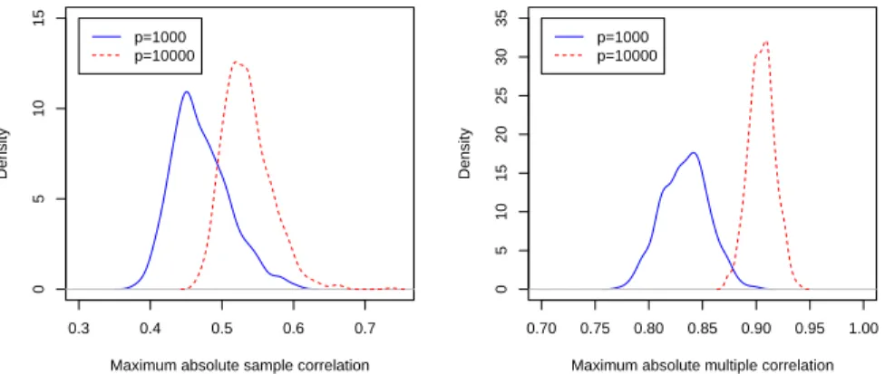
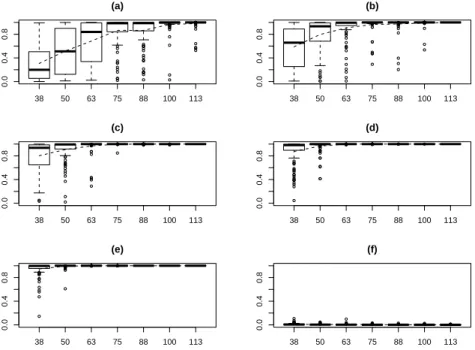
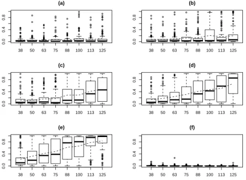
Figure 2.1 shows the distributions of marginal inclusion probabilities for the five true predictors and one false predictor. It is easy to see that as n increases, the marginal inclusion probabilities of the true predictors converge toward 1, while the marginal inclusion probability of the false predictor stays close to 0. This confirms the sure screening property of the marginal inclusion probability as established in Theorem 2.1.3. Figure 2.2 shows that the probability of the MAP model catching the true model increases with n. This confirms Theorem 2.1.4 that the MAP model is consistent. A comparison of Figure 2.1 and Figure 2.2 show that from the perspective of variable selection, the marginal inclusion probability may work better than the MAP model, as the former seems to converge faster than the latter.
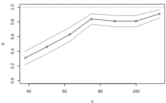
A further simulation study is conducted here to study the stability of our approach when the multicollinearity is extremely strong. Instead of 0.25, we let the pairwise correlation to be 0.9, and let n increase from 30 to 125, whilst keep the other settings unchanged. Under such extremely high multicollinearity, the MAP model almost never catch the true model. However, as showed in figure 2.3, the trend of increasing marginal inclusion probabilities for the true predictor is still clear.
2.3.1.0.2 Example 2 This example illustrates the SaM approach. It consists of 100 simulated data sets, each consisting of n = 150 observations and pn = 1000
predictors. For each data set, the design matrixX was generated from a multivariate normal distribution. The first 100 columns of X are mutually correlated with an equal correlation coefficient of 0.25, and independent of the rest 900 columns. The rest 900 columns are mutually independent. The first three columns were chose as
● ● ● ● ● ● ● ● ● ● ● ● ● ● ● ● ● ● ● ● ● ● ● ● ● ● ● ● ● ● ● ● ● ● ● ● ● ● ● ● ● ● ● ● ● ● ● ● ● ● ● ● ● ● ● ● ● ● ● ● ● 38 50 63 75 88 100 113 0.0 0.4 0.8 (a) ● ● ● ● ● ● ● ● ● ● ● ● ● ● ● ● ● ● ● ● ● ● ● ● ● ● ● ● ● ● ● ● ● ● ● ● ● ● ● ● ● ● ● ● ● ● ● ● ● ● ● ● ● ● ● ● ● ● ● ● ● ● ● ● ● ● ● ● ● ● ● ● ● ● ● ● ● ● ● ● 38 50 63 75 88 100 113 0.0 0.4 0.8 (b) ● ● ● ● ● ● ● ● ● ● ● ● ● ● ● ● ● ● ● ● ● ● ● ● ● ● ● ● ● ● ● ● ● ● ● ● ●●●● ● ● ● ● ● ● ● ● ● ● ● ● ● ● ● ●●●●●●●●●●●●●●●●●●●●●●●● ●●●● 38 50 63 75 88 100 113 0.0 0.4 0.8 (c) ● ● ● ● ● ● ● ● ● ● ● ● ● ● ● ● ● ● ● ● ● ● ● ● ● ● ● ● ● ● ● ● ● ● ● ●●●●●●●●●●●●●●●●●●● ●●●●●●●●●●●●●●●●●●●●●● ●●● ● 38 50 63 75 88 100 113 0.0 0.4 0.8 (d) ● ● ● ● ● ● ● ● ● ● ● ● ● ● ● ● ● ● ● ● ● ● ● ● ● ● ● ● ● ● ● ● ● ● ● ● ●●●●●●●●●●●●●●●●●●● ●●●●●● 38 50 63 75 88 100 113 0.0 0.4 0.8 (e) ● ● ● ● ● ● ● ● ● ● ●●●●●●●● ● ● ● ● ● ● ● ● ●●●●●●●● ●●●●●●● ●●●●●● ●●●●● 38 50 63 75 88 100 113 0.0 0.4 0.8 (f)
Figure 2.1: Simulation results for marginal inclusion probabilities. The six plots showed in this figure, (a)-(f), present the distributions of marginal inclusion prob-abilities of six predictors with the true regression coefficients 0.7, 0.9, 1.1, 1.3, 1.5 and 0, respectively. In each plot, the seven boxplots are for the sample size n = 38,50,63,75,88,100,113, respectively. Each boxplot shows the distribution of the marginal inclusion probabilities of one predictor calculated from 100 simulated data sets. The dashed line in each plot shows the mean value of the marginal inclu-sion probabilities.
● ● ● ● ● ● ● 40 60 80 100 0.0 0.2 0.4 0.6 0.8 1.0 n p
Figure 2.2: Simulation results for MAP model. The plot give the estimated proba-bility that the MAP model coincides with the true model. For each value of n, the probability was estimated from 100 simulated data sets. The dashed lines show the 95% confidence interval of the probability.
the true predictors with the regression coefficients being 1.5, 3.0 and 4.5, respectively. We randomly split each data set into 50 subsets with s = 20. In stage I, the predictors are iteratively selected twice for each subset. Each run of SAMC consists of 270× |s|iterations, where the first 20× |s|iterations were for the burn-in process, and s can be a subset directly split from the full data set or a remainder of a subset containing only unselected predictors. The gain factor sequence was set as ak = 10|s|/max{10|s|, k}, where k indexes the number of iterations of SAMC. The
prior hyperparameter ¯s was set to 20. The FDR level was set toα1 = 0.15, which is
relatively large such that the variable selection is liberal and thus reducing the risk of losing important true predictors. In stage II, SAMC was run for the aggregated data set with 270×pn iterations, where the first 20×pniterations were for the
burn-in process. The gaburn-in factor sequence was set as ak = 10pn/max{10pn, k}, where k
indexes the number of iterations of SAMC. The prior hyperparameter ¯rn was set to
● ● ● ● ● ● ● ● ● ● ● ● ● ● ● ● ● ● ● ● ● ● ● ● ● ● ● ● ● ● ● ● ● ● ● ● ● ● ● ● ● ● ● ● ● ● ● ● ● ● ● ● ● ● ● ● ● ● ● ● ● ● ● ● ● ● ● ● ● ● ● ● ● ● ● ● ● ● ● ● ● ● ● ● ● ● ● ● ● ● ● ● ● ● ● ● 38 50 63 75 88 100 113 125 0.0 0.4 0.8 (a) ● ● ● ● ● ● ● ● ● ● ● ● ● ● ● ● ● ● ● ● ● ● ● ● ● ● ● ● ● ● ● ● ● ● ● ● ● ● ● ● ● ● ● ● ● ● ● ● ● ● ● ● ● ● ● ● ● ● ● ● ● ● ● ● ● ● ● ● ● ● ● ● ● ● ● ● ● ● ● ● ● ● ● ● ● ● ● ● ● ● ● ● ● ● ● ● ● ● ● ● ● ● ● 38 50 63 75 88 100 113 125 0.0 0.4 0.8 (b) ● ● ● ● ● ● ● ● ● ● ● ● ● ● ● ● ● ● ● ● ● ● ● ● ● ● ● ● ● ● ● ● ● ● ● ● ● ● ● ● ● ● ● ● ● 38 50 63 75 88 100 113 125 0.0 0.4 0.8 (c) ● ● ● ● ● ● ● ● ● ● ● ● ● ● ● ● ● ● ● ● 38 50 63 75 88 100 113 125 0.0 0.4 0.8 (d) ● ● ● ● ● ● ● ● ● ● ● ● ● ● ● ● ● ● ● ● ● ● ● ● ● ● ● ● ● ● ● ● ● ● 38 50 63 75 88 100 113 125 0.0 0.4 0.8 (e) ● ● ● ● ● ● ● ●●●●●● ● ● ● ● ● ● ● ● ● ● ● ● ● ● ● ●●●●●●●● ●●●●●●●●● ●●●●●●● ●●●●●●●●●● ●● ● ● ● ● ● ● ● ● 38 50 63 75 88 100 113 125 0.0 0.4 0.8 (f)
Figure 2.3: Simulation results for marginal inclusion probabilities under extremely high multicollinearity. The six plots showed in this figure, (a)-(f), present the distri-butions of marginal inclusion probabilities of six predictors with the true regression coefficients 0.7, 0.9, 1.1, 1.3, 1.5 and 0, respectively. In each plot, the seven boxplots are for the sample size n = 38,50,63,75,88,100,113 and 125, respectively. Each boxplot shows the distribution of the marginal inclusion probabilities of one predic-tor calculated from 100 simulated data sets. The dashed line in each plot shows the mean value of the marginal inclusion probabilities.