POUR L'OBTENTION DU GRADE DE DOCTEUR ÈS SCIENCES
acceptée sur proposition du jury: Prof. C. N. Jones, président du jury Prof. H. Bourlard, Dr B. Caputo, directeurs de thèse
Prof. V. Murino, rapporteur Prof. D. Skocaj, rapporteur Prof. J.-Ph. Thiran, rapporteur
SALIENCY-BASED REPRESENTATIONS AND
MULTI-COMPONENT CLASSIFIERS FOR VISUAL SCENE
RECOGNITION
THÈSE N
O6424 (2014)
ÉCOLE POLYTECHNIQUE FÉDÉRALE DE LAUSANNE
PRÉSENTÉE LE 24 NOVEMBRE 2014À LA FACULTÉ DES SCIENCES ET TECHNIQUES DE L'INGÉNIEUR LABORATOIRE DE L'IDIAP
PROGRAMME DOCTORAL EN GÉNIE ÉLECTRIQUE
Suisse PAR
The journey of a thousand miles begins with one step. — Tao Te Ching
Acknowledgements
Few things are as enjoyable as writing an acknowledgment section, as this is a moment in which one has the opportunity to express gratitude to all those who generously contributed to the successful completion of a big piece of work.
First of all, I am very grateful to my supervisor Prof. Barbara Caputo for giving me the opportu-nity to carry out my doctoral studies at Idiap and EPFL. Barbara, I am thankful for your steady support throughout my doctoral journey and for the scientific freedom and trust that you have always granted me. Your pragmatic and open-minded attitude and guidance were and are a source of inspiration for my personal and professional growth. A big thank goes also to Prof. Francesco Orabona, for his support and guidance with his admirable technical mastery during several stages of my scientific journey. Thank you Francesco.
I would like to take this occasion to thank my thesis director Prof. Hervé Bourlard, as well as Prof. Jean Philippe Thiran, Prof. Vittorio Murino, Prof. Danijel Sko˘caj and Prof. Colin Jones for accepting to be part of my examination jury and for kindly taking the time to read my thesis in their busy schedule. I am also grateful to the Idiap system group and the Idiap and EPFL secretariats for their indispensable help in infinitely many occasions.
Amongst the most-rewarding non-scientific privileges of a Ph.D. student at Idiap and EPFL is the opportunity to meet talented people from all over the world, driven here by a thirst for knowledge, a pronounced curiosity and a sharp analytical mind ; each of them carrying his background, homeland culture, colors and tastes. I would thus like to thank the many people I have met here and who have greatly enriched my days : thanks to Laurent for the many great moments in the wilds, the many dinners and the many musical sessions ; thanks to Deepu for all the nice moments together, for introducing and hosting me into his family and for showing me the magic of his homeland, Kerala ; thanks to Leo for just being the funny and generous mate he naturally is ; thanks to Jagan for all the inspiring discussions about life, God and philosophy ; thanks to Thomas and Vincent for introducing me to climbing and slacklining ; thanks to Anindya for the many stimulating discussions about almost everything ; thanks to Ilja for the many stimulating discussions about almost only machine learning, for his company in Chicago and, together with Novi, for proof-reading part of this thesis ; thanks to Arjan for his support and his friendship ; thanks to Nesli, Ufuk, Rémi, Gwénolé, Marc, Vicky, Kai, Manuel, Roy, Harsha, Paul, Alexandros, Alex, Samira, Mohammad, Majid, David, Raphael, Ramya, Lakshmi, Sriram, Kenneth, Gülcan, Rui, PE, Cijo, Pranay, Dayra, Petr, Cosmin,
Charles, Nikos, Nik, Nicolae, Hugo, Paco, Tatiana, Serena, Gigi, Roger, Dinesh, Phil and Hari for organizing and participating to many funny social events, filling Martigny with their cheerful spirit. Thanks also to Michel for struggling to teach us some French and for sharing with us some bits of the special Valaisan life style.
A very special thanks goes to Ivana. I really do not exaggerate if I say that without her I would not be writing these words now. Her presence, trust and support in the most difficult moments provided me the drive and lift to continue and succeed. As I used to say, I should have written an entire acknowledgement section just for her.
Finally, it is needless to say I am infinitely grateful to my parents and to my full family for everything they did for me.
Abstract
Visual scene recognition deals with the problem of automatically recognizing the high-level semantic concept describing a given image as a whole, such as the environment in which the scene is occurring (e.g. a mountain), or the event that is taking place (e.g. a rock climbing event). Scene categories, especially those related to man-made places and events, present high degrees of intra-class variability and inter-class similarity, which in turn require robust and discriminative recognition systems. An additional requirement for potential applications, such as vision-based spatial reasoning for mobile robots, is efficiency of the classification procedure. The objective of this thesis is to address these challenges, by proposing suitable image representations and classification algorithms.
The first part of the thesis focuses on the representation task. We propose a bottom-up image descriptor capturing perceptually coherent structures independently of their position. In particular, our method separately pools features extracted from two perceptually different image regions : the most salient region and the remaining non-salient one. By complementing thisSaliency-driven Perceptual Pooling(SPP) with an ad-hoc spatial pooling operation, we obtain compact and robust image representations, particularly suited for indoor and sports scenes.
The second part of the thesis is concerned with the classification step. We propose an efficient multi-component classification algorithm, namedMulticlass Latent Locally Linear SVM(ML3), able to automatically learn a set of sub-categorical linear models for each class, in a principled latent SVM framework. By linearly combining the sub-categorical models with sample and class specific weights, ML3 is able to efficiently learn smooth non-linear decision boundaries, competitive with those obtained by Gaussian kernel SVMs. ML3 also shows very competitive trade-offs between training time and performance, while ensuring high efficiency of the prediction phase.
In the last part of the thesis, we use the ML3 algorithm to improve the efficiency and per-formance of a recently proposed image classification algorithm, namedNBNN, designed to cope with classes with a large diversity. Specifically, we show how with a modification of the NBNN scoring function it is possible to use ML3 to learn a discriminative and compact set of prototypical local features for each class, and thus avoid the extensive Nearest Neighbor search used by NBNN. The resulting algorithm, namedNBNL, greatly reduces the memory requirements and testing complexity of NBNN, while significantly improving its performance. The approaches proposed in this thesis effectively exploit the spatial, salient and task-driven structures present in the images, producing compact representations and relatively efficient
classification procedures.The SPP representations provide competitive scene recognition performances when coupled with non-linear kernels, while the ML3 algorithm can be used to partially fill the gap between linear and non-linear kernels. Although the performance of NBNN-based methods on scene recognition tasks is still below the one obtained by traditional SVM-based approaches, the proposed NBNL algorithm reduces the performance gap, while significantly speeding up the testing phase. Experiments on three publicly available scene recognition datasets (MIT-Indoor-67, 15-Scenes and UIUC-Sports) show the value of the proposed approaches.
Key words : visual scene recognition, saliency maps, feature pooling, multi-component classifi-cation, multi-class classificlassifi-cation, locally linear SVM, latent SVM, naive Bayes nearest neighbor
Résumé
La reconnaissance visuelle des scènes consiste à déterminer le concept sémantique de haut niveau qui décrit une image dans son ensemble, comme l’environnement dans lequel la scène se dresse (e.g. une montagne), ou l’événement qui s’y déroule (e.g. une activité d’escalade). Les différentes catégories de scènes, en particulier celles liées aux endroits et événements créés par l’homme, présentent une variabilité intra-classe et une similarité inter-classe très impor-tante, ce qui nécessite des systèmes de reconnaissance robustes et discriminatifs. Un besoin supplémentaire pour de possibles applications, comme le raisonnement spatial en utilisant l’information visuelle pour des robots mobiles, est l’efficacité de la procédure de classification. L’objectif de cette thèse est de résoudre ces problèmes, en proposant des représentations d’images et des algorithmes de classification adaptés.
La première partie de cette thèse porte principalement sur l’étape de représentation. Nous proposons un descripteur d’image de bas en haut, qui capture les structures cohérentes sur le plan perceptif indépendamment de leur position dans l’image. En particulier, notre méthode met en commun les caractéristiques extraites de deux régions différentes sur le plan perceptif séparément : la région la plus saillante et l’autre région non saillante. En complétant cette mise en commun perceptive guidée par la saillance (SPP) avec une opération de mise en commun spatiale ad hoc, nous obtenons des représentations d’images compactes et robustes, particulièrement adaptées aux scènes d’intérieur et de sport.
La deuxième partie de cette thèse concerne l’étape de classification. Nous proposons un algorithme efficace de classification à plusieurs composants, dénommé SVM multi-classe latent localement linéaire (ML3), capable d’apprendre automatiquement un ensemble de modèles linéaires sous-catégoriques pour chaque classe, dans un cadre reposant sur un SVM latent. En combinant linéairement les modèles sous-catégoriques avec des pondérations liées aux échantillons et aux classes, ML3 est en mesure d’apprendre efficacement des frontières de décision lisses et non-linéaires, qui rivalisent avec celle obtenues par des SVMs à noyau gaussien. ML3 montre également un équilibre très intéressant entre durée d’apprentissage et performance, tout en assurant une bonne efficacité lors de l’étape de prédiction.
Dans la dernière partie de cette thèse, nous utilisons l’algorithme ML3 pour améliorer l’ef-ficacité et la performance d’un algorithme de classification d’images récemment proposé, NBNN, qui a été conçu de façon à s’adapter à des classes avec une très grande variabilité. Plus particulièrement, nous montrons comment il s’avère possible, en modifiant la fonction de score du NBNN, d’utiliser ML3 pour apprendre un ensemble discriminatif et compact de caractéristiques locales prototypique pour chaque classe, et, ainsi, d’éviter de recourir à
la vaste recherche des plus proches voisins utilisée par NBNN. L’algorithme qui en résulte, dénommé NBNL, réduit grandement les besoins en mémoire et la complexité de l’évaluation par rapport au NBNN, tout en améliorant significativement les performances.
Les approches proposés dans cette thèse exploitent efficacement les structures spatiales, sail-lantes ainsi que celles destinées à des tâches spécifiques, présentes dans les images, générant ainsi des représentations compactes et des procédures de classification relativement efficaces. Les représentations SPP fournissent des performances compétitives en reconnaissance de scènes lorsqu’elles sont associées avec des noyaux non-linéaires, tandis que l’algorithme ML3 peut être utilisée pour combler partiellement l’écart entre noyaux linéaires et non-linéaires. Bien que les performances en reconnaissance de scènes des méthodes reposant sur NBNN soient encore en dessous de celles obtenues avec les approches classiques à base de SVM, l’algorithme NBNL proposé réduit cet écart de performance, tout en accélérant significa-tivement l’étape de classification. Des expériences conduites sur trois bases de données de reconnaissance de scènes accessibles au public (MIT-Indoor-67, 15-Scenes et UIUC-Sports) révèlent l’utilité des méthodes proposées.
Mots clefs : reconnaissance visuelle des scènes, cartes de saillance, mise en commun de carac-téristiques, classification à plusieurs composants, classification multi-classe, SVM localement linéaire, SVM latent, classification naïve bayésienne par plus proches voisins
Contents
Acknowledgements v
Abstract (English) vii
Résumé (Français) ix
List of figures xviii
List of tables xix
Glossary xx
Notation xxi
1 Introduction 1
1.1 Motivation . . . 1
1.2 Statement of the problem and challenges . . . 2
1.3 Objectives and approach . . . 4
1.4 Contributions and structure . . . 6
1.5 References . . . 8 2 Related Works 9 2.1 Datasets . . . 11 2.2 Descriptor Extraction . . . 15 2.2.1 Low-level descriptors . . . 15 2.2.2 Mid-level descriptors . . . 17 2.2.3 High-level descriptors . . . 20 2.3 Image signature . . . 22 2.3.1 Spatial analysis . . . 23 2.3.2 Saliency analysis . . . 25 2.3.3 Pooling . . . 26 2.4 Classification . . . 27 2.4.1 Monolithic Classifiers . . . 27 2.4.2 Multi-component Classifiers . . . 29 2.4.3 Sub-categories and multiple components in object and scene recognition 33
3 Spatial and Saliency-driven Representations of Visual Scenes 35
3.1 Introduction . . . 35
3.2 Related works . . . 37
3.3 The proposed approach . . . 39
3.3.1 Saliency-driven Perceptual Pooling (SPP) . . . 40
3.3.2 Task-driven Spatial Pooling (TSP) . . . 43
3.3.3 Integrating Saliency-driven and Task-driven pooling . . . 44
3.4 Experiments . . . 44
3.4.1 Experimental setup . . . 44
3.4.2 Empirical analysis of the method . . . 45
3.4.3 Experimental results . . . 51
3.5 Discussion . . . 57
4 ML3 - A Multiclass Latent Locally Linear SVM algorithm 59 4.1 Introduction . . . 60
4.2 Related works . . . 62
4.3 Preliminaries . . . 63
4.3.1 Latent SVM . . . 63
4.3.2 The Constrained Concave Convex (CCCP) procedure. . . 65
4.3.3 Locally Linear SVMs . . . 65
4.4 The proposed approach . . . 66
4.4.1 Locally Linear Coding (L2C) . . . 66
4.4.2 Multiclass Latent Locally Linear SVM (ML3) . . . 71
4.5 Explicit feature maps and visualizations . . . 77
4.6 Hyper-parameters setting . . . 80 4.7 Experiments . . . 82 4.7.1 Benchmark datasets. . . 84 4.7.2 Character recognition. . . 87 4.7.3 Scene Recognition . . . 93 4.8 Discussion . . . 97
5 Patch-based classification of Visual Scenes 99 5.1 Introduction . . . 99
5.2 Related works . . . 100
5.3 The NBNL approach . . . 102
5.3.1 The NBNN algorithm . . . 102
5.3.2 The NBNL decision rule . . . 103
5.3.3 Learning the NBNL prototypes . . . 105
5.4 Experiments . . . 106
5.4.1 Single-scale experiments . . . 107
5.4.2 Multi-scale experiments . . . 109
5.4.3 Experiments with Horizontal and Saliency-driven Perceptual Pooling . . 112
Contents
6 Conclusion 115
6.1 Achievements . . . 115 6.2 Discussion, limitations and future work . . . 117
A Mathematical proofs 119
B Visualizations 125
Bibliography 126
List of Figures
1.1 Examples of scene categories exhibiting intra-class variability. Top: structural variability in images from the scene category “bocce”. Bottom: view-point variability in images from the scene category “coast”. . . 2 1.2 Examples of scenes exhibiting high degrees of inter-class similarity. Images
annotated with “living” belong to the scene category “living room”, while scenes annotated with “dining” belong to the scene category “dining room”. . . 3 1.3 Challenges of the scene recognition problem. . . 4 2.1 The general scene recognition pipeline considered in this thesis. . . 10 2.2 Example images from the 67 classes of the MIT-Indoor-67 dataset, organized by
scene group. (Adapted from Quattoni and Torralba [2009]) . . . 12 2.3 Example of images from the classes of the 15-Scenes dataset. . . 13 2.4 Example of images from the classes of the UIUC-Sports dataset. . . 14 2.5 Visualization of the Spatial Pyramid Matching approach. (Adapted from
Lazeb-nik et al. [2006]) . . . 23 3.1 Saliency-driven segmentation of images from office and kindergarden
cate-gories (MIT-Indoor-67 dataset [Quattoni and Torralba, 2009]). For each image, a saliency map [Itti et al., 1998] was computed and then then segmented in two regions: the most and least salient 50%. Dark areas correspond to low saliency regions. . . 36 3.2 Saliency-driven segmentation of images from badminton and snowboarding
cat-egories (UIUC-Sports dataset [Li and Fei-Fei, 2007]). For each image, a saliency map [Itti et al., 1998] was computed and then then segmented in two regions: the most and least salient 50%. Dark areas correspond to low saliency regions. . 37 3.3 The scene recognition pipeline proposed in this Chapter. The component of the
pipeline related to the main contribution of this Chapter is highlighted by a thick border. . . 38 3.4 Top: visualization of the 128 SIFT Independent Components, summed over the
8 orientations; white pixels correspond to high ICA (rectified) weights for the gradients in the corresponding area of the SIFT patches. Bottom: Computation of a SIFT saliency map and resulting segmentation usingl =2 regions and
3.5 Histograms obtained (withl=2 regions andλ1=λ2=12) using different pooling
techniques and number of non-zero visual words in each of the two halves of the histograms: non-salient (NS) and salient (S), left (L) and right (R), up (U) and down (D). . . 43 3.6 Left: average number of non-zero visual words in each part of the representation,
as obtained with different pooling techniques withl=2. For Horizontal pooling Part 1 is the top part of the image, for Vertical pooling Part 1 is the left part of the image, while for SPP Part 1 is the non-salient region. Right: average overlap (in % of the number of pixels) between salient regions and horizontal/vertical patches, compared to the average overlap of the salient regions obtained with the Itti’s and the SIFT SPP representations. The plots are obtained withλ1=12on the
MIT-Indoor-67 dataset (top), the 15-Scenes dataset (center) and the UIUC-Sports dataset (bottom). . . 46 3.7 Performance obtained by the saliency-driven pooling approaches when varying
the percentage of the image descriptors that are assigned to the non-salient region. The results are provided for single and multiresolution, Itti’s and SIFT SPP representations, on the MIT-Indoor-67 (left), the 15-Scenes (center) and the UIUC-Sports (right) datasets. For visualization purposes we also plot the average performance of the four SPP descriptors. . . 47 3.8 Performance obtained by separately using the single-resolution features pooled
over the salient and non-salient region, and when concatenating the two rep-resentations. The mass coefficientλ1is varied from 0.1 to 0.9 and results are
reported for the MIT-Indoor-67 (top), the 15-Scenes (middle) and the UIUC-Sports (bottom) datasets. . . 49 3.9 Relative performance of different pooling strategies w.r.t. the Horizontal baseline
(withl=2), using single-resolution descriptors on the MIT-Indoor-67 (left), the 15-Scenes (center) and the UIUC-Sports (right) datasets. “Horizontal3” stands for the horizontal bands pooling withl=3 andλ1=λ2=λ3=13. . . 50
3.10 Performances of the different pooling strategies on the MIT-Indoor-67 dataset. 52 3.11 Example of images from some of the classes in each scene group of the
MIT-Indoor-67 dataset. . . 52 3.12 Accuracy obtained when using single-resolution descriptors to classify the
im-ages from MIT-Indoor-67 with respect to which of the five scene groups (Store, Home, Public place, Leisure, or Working place) they belong to. . . 53 3.13 Analysis of the performance of the spatial and saliency-driven pooling approaches
on the five scene groups of the MIT-Indoor-67 dataset. . . 54 3.14 Performances on the 15-Scenes dataset. . . 55 3.15 Performances on the UIUC-Sports dataset. . . 56 4.1 The scene recognition pipeline proposed in this Chapter. The component of the
pipeline related to the main contribution of this Chapter is highlighted by a thick border. . . 62
List of Figures
4.2 Training sequence on a synthetic XOR dataset, using two components andp=1. For each experiment we color encode the sample-to-component assignments (first row of the first column), with the RGB values set according to the first three components ofβWyiˆ (xi). We also plot a 2D projection ofψ
³
xi,βWyiˆ (xi)
´
with the ground-truth label color encoded in red and cyan (second row of the first column of each experiment). In the third row of the first column we plot the resulting decision boundary in the original input space, with the ground-truth label color encoded again in red and cyan. Finally, on the second column of each experiment we plot the normalized Gramian matrices computed using the original data (first row), usingψ³xi,βWyiˆ (xi)
´
(second row) and difference between the latter and the former (third row). In the Gramian matrices the samples are ordered according to their ground-truth labels. . . 78 4.3 Training sequence on the Banana dataset, using three components andp=1.
For each experiment we color encode the sample-to-component assignments (first row of the first column), with the RGB values set according to the first three components ofβWyiˆ (xi). We also plot a 2D projection ofψ
³
xi,βWyiˆ (xi)
´
with the ground-truth label color encoded in red and cyan (second row of the first column of each experiment). In the third row of the first column we plot the resulting decision boundary in the original input space, with the ground-truth label color encoded again in red and cyan. Finally, on the second column of each experiment we plot the normalized Gramian matrices computed using the original data (first row), usingψ³xi,βWyiˆ (xi)
´
(second row) and difference between the latter and the former (third row). In the Gramian matrices the samples are ordered according to their ground-truth labels. . . 79 4.4 Effect of varying the parameterpin the set {1, 2, 1000}, usingm=5 on Banana
dataset. As in Figures 4.2 and 4.3, for each experiment we color encode the sample-to-component assignments, we plot a 2D projection ofψ(xi,βWyiˆ(xi)),
the resulting decision boundary and the normalized Gramian matrices com-puted using the original data, usingψ(xi,βWyiˆ (xi)) and difference between the
latter and the former. . . 81 4.5 Performance on USPS, when varying bothpand the number of componentsm. 82 4.6 Performance of the L2C coding on the UCI benchmark datasets. Left: average
test error rate and ranking, varyingpbetween 1 and 2. Right: average ranking, varyingpbetween 1 and 2. . . 86 4.7 Results varying the number of iterations on the USPS, LETTER, MNIST and
COVTYPE datasets. Top: error rates on usingm=100. The curves related to OCC for LETTER and COVTYPE are obtained withm=16 andm=54, due to the limitations of the encoding. Bottom: value of the objective function of ML3 with m=100. . . 90 4.8 Error rates varying the number of componentsmon the USPS, LETTER, MNIST
4.9 Error rates varying the parameterpof the ML3 algorithm on the USPS, LETTER, MNIST and COVTYPE datasets. . . 91 4.10 Error rate versus training time on the USPS, LETTER, MNIST and COVTYPE
datasets. . . 92 4.11 Average test error rate on the ISR dataset, varying the number of componentsm. 94 4.12 Average accuracy on MIT-Indoor-67 (left), 15-Scenes (center) and UIUC-Sports
(right), withm=8 components. . . 95 5.1 The scene recognition pipeline proposed in this Chapter. The component of the
pipeline related to the main contribution of this Chapter is highlighted by a thick border. . . 101 5.2 Left: performance of the NBNL algorithm varying the number of prototypes,
w.r.t. the NBLL baseline (using a One-Vs-All linear SVM). Right: performances of our method and several other baselines with an asymmetric sampling strategy (sub-sampling the patches only from the training images). All the results are obtained using single-scale SIFT features. Results on the top are obtained on the 15-Scenes dataset. Results on the bottom are obtained on the UIUC-Sports dataset. . . 108 5.3 Visualization of the classification results on images of the UIUC-Sports (top) and
the 15-Scenes (bottom) datasets. Each image is titled with its ground-truth label, while in green, blue and red are visualized the top-scoring SIFT patches for the three top-scoring classes (from lowest to highest) of each image. . . 110 5.4 Scene recognition performance obtained by applying the SPP approach
de-scribed in Chapter 3 to the NBNL algorithm. Results marked with the keyword multiare obtained using a multi-scale setup. The other results are obtained using the single scale setup. . . 113 B.1 Visualizations of the segmentation masks obtained using Itti Saliency on images
List of Tables
2.1 List of scene recognition publications and datasets used. From the list we exclude
the publications in which a new dataset was proposed. . . 11
3.1 Performance comparison with previous approaches using a single image descrip-tor. For each approach we also report the dimensionality of the representation used. . . 57
4.1 Average test error rate and ranking on the UCI benchmark datasets. . . 84
4.2 Average training times (in seconds) on the UCI benchmark datasets. . . 85
4.3 Average testing times (in seconds) on the UCI benchmark datasets. . . 85
4.4 Error rate and associated training and testing time (in seconds) of different algorithms. The results taken from other papers are reported with the citation. The results for multi-component approaches (LLSVM, OCC, L2C, AMM, ML3, ML3+I) are obtained by training the algorithms for 30 epochs (or CCCP iterations) withp=1.5 andm=80 for USPS,m=16 for LETTER,m=90 for MNIST,m=54 for COVTYPE. . . 87
4.5 Training times, testing times and size of the model for Linear SVM, ML3 and Gaussian kernel SVM, as measured using multiresolution Horizontal + SPP image signatures. . . 96
4.6 Performance comparison with previous studies applying multi-component ap-proaches to scene recognition problems. For each approach we also report the number of componentsmand the number of times the multi-component model has to be evaluated to produce the final image classification. . . 97
5.1 Results of NBNL using multi-scale SIFT features, compared to NBNN baselines on the same feature set, NBNN results reported in the literature (with citation) and two SLC-BoW algorithms on the same feature set (top). . . 111
5.2 Comparison of the results of NBNL + Horizontal + SPP to other NBNN ap-proaches using spatial information. . . 113
BoW Bag of visual Words
CCCP Constrained Concave Convex Procedure
ICA Independent Component Analysis
LHS Left-Hand Side
LLSVM Locally Linear SVM
MAP Maximum A-Posteriori
ML3 Multiclass Latent Locally Linear SVM
NN Nearest Neighbor
NBNL Naive Bayes Non-linear Learning
NBNN Naive Bayes Nearest Neighbor
PCA Principal Component Analysis
RHS Right-Hand Side
SGD Stochastic Gradient Descent
SIFT Scale Invariant Feature Transform
SPM Spatial Pyramid Matching
SPP Saliency-driven Perceptual Pooling
Notation
Ati j a matrix (indexed for some purpose) ai j a vector (indexed for some purpose)
¡
ai j¢
k thek-th entry of the vectorai j
a a scalar
R a set
f(·) a real-valued, vector-valued, or matrix-valued function A> the transpose of the matrixA
Tr (A) the trace of the matrixA
A·B the Frobenius inner product between the matricesAandB
kAkF the Frobenius norm of the matrixA
kakp thep-norm of the vectora
a+ the elementwise maximum between the vectoraand 0 a≥b a vector inequality which holds i.i.f.ai≥bi,∀i
a≥b a vector inequality which holds i.i.f.ai≥b,∀i
|a| the absolute value ofa
|a|+ the maximum betweenaand 0
1¡
p¢
the indicator function of the predicate p (an equation, or an inequality)
Except when explicit from the context, we also make use of the following naming conventions: X ⊆Rd the input space
Y the output space
(x,y) an (input,output) sample
d the dimensionality of the input space
n the number of training samples
c the number of classes in a given classification problem
m the number of components in a given model
r the number of local descriptors in a given image k the number of visual words in a BoW model
1
Introduction
1.1 Motivation
With the advent and widespread commercialization of inexpensive digital cameras, large amounts of digital images are being generated every day. Computers have become the main mean of storage and fruition of images, and the necessity to efficiently group, categorize and search this vast quantity of digital images has become a critical matter. Hence, efforts in developing various low and high-levelcomputer visiontechniques, which may help in this direction come with no surprise. Techniques such as color analysis and face detection or recognition have already been deployed in digital photo organizers and digital cameras. Still, there is a growing need for methods able to reliably and efficiently provide additional high-level information about the captured images. One basic type of high-level information that can be used to facilitate the management of large databases of images is the one regarding the global environment in which each image is captured. For example, one may be interested in retrieving all the images in which a given person is appearing in a mountain scenario, or in an office environment. In order to provide such high-level annotations of the images, it is thus necessary to design computer vision algorithms able to efficiently recognize these concepts. Parallel to the ubiquitous diffusion of digital cameras, recent years have also seen the break-through of mobile robotics into the consumer market. Domestic robots have become in-creasingly common and are now extensively used to perform simple tasks, such as vacuum cleaning, or cutting the grass in the garden. Major automobile manufacturers and technology companies have already announced short-term plans to commercialize vehicles making use of cameras, radar and other sensors to assist the driver, or even autonomously conduct the passengers. In order to simplify the communications between humans and these artificial agents, and to enable a high-level reasoning using abstract spatial concepts, the human repre-sentation of space should also be understood and reproduced by artificial agents. For example, a domestic robot may be asked to “clean the bathroom”, while a car may be asked to “stop at the gas station”, or at “the parking area”. Consequently, a robot’s definition of “bathroom”, or “parking area” should point to the same set of places that a human would recognize as such.
Figure 1.1 – Examples of scene categories exhibiting intra-class variability. Top: structural variability in images from the scene category “bocce”. Bottom: view-point variability in images from the scene category “coast”.
1.2 Statement of the problem and challenges
In computer vision, the task of automatically annotating a single image with the categorical label that best describes the scene as a whole is known asscene recognition. As opposed to objects, scenes are mainly characterized as places in which humans can move [Oliva and Torralba, 2001]. This definition can be extended to include events, such as sports activities [Li and Fei-Fei, 2007] (e.g. a “sailing” scene, or a “croquet” scene).
The most important challenges in scene recognition come from the complexity of the concepts to be recognized and the variability of the conditions in which the images are captured. Scenes from the same category may often look different, while scenes from different categories may look similar. We refer to the variability in the appearance of images within a single scene category asintra-class variability, while the similarity of images belonging to different categories is referred to asinter-class similarity. Besides intra-class variability and inter-class similarity, an additional challenge for scene recognition, coming from the application domain, is due toefficiency requirements.
Intra-class variability is mainly due to two factors:
1. Structural complexity and variability.Scenes are complex high-level concepts, in turn composed of several complex parts, whose number, types and configurations cannot be fixeda priori. Take for example the category “office”. An office would likely contain desks and chairs, but their number and spatial arrangement may vary from instance to instance. Moreover, additional parts, such as computers, printers, telephones, lamps, shelves, books, white-boards, plants and windows may or may not be present.
2. View-point variability.Scenes can look very different from different points of view. This is especially true for indoor scenes, where the distance between the subject of the picture
1.2. Statement of the problem and challenges
dining living dining living
Figure 1.2 – Examples of scenes exhibiting high degrees of inter-class similarity. Images anno-tated with “living” belong to the scene category “living room”, while scenes annoanno-tated with “dining” belong to the scene category “dining room”.
and the observer is often very low. For example, a bedroom may be captured from a viewpoint in which the full bed is visible, or from the opposite viewpoint, in which only other objects such as a television, wardrobes, mirrors and desks are fully visible. Due to the high levels of visual variability, images belonging to a certain scene category may cluster into so called visualsub-categories. A visual sub-category consists of images from the same scene category having a common perceptual appearance.
It is to be noted that the structural variability of scene categories is higher than for object categories [Ehinger, 2013]. Take, for example, object categories such as car, dog, washing machine, or mobile phone. Although there might be sub-categories (e.g. “smart-phone” vs “old-generation mobile phone”) and the final appearance may be very different, it is not difficult to think of a prototypical set of parts with a prototypical spatial configuration for each object category, or sub-category (e.g. two wheels in front, two wheels on the back, a body above the wheels and several windows above the body, for the category “car”). The same reasoning cannot be easily reproduced for many scene categories, as the “office” category described above, other indoor categories, or even for sport scenes. A match of “bocce”, for example, can be played indoor, as well as outdoor, on a proper framed field, on the grass, or even on the beach. Moreover, the exact number of players, bowls and their relative positions may vary continuously from image to image (see Figure 1.1).
In Figure 1.1 we report some examples of images from the scene categories “bocce” and “coast”, illustrating the effects of structural and view-point variability, respectively. As it can be seen, images from the category “bocce” do present a considerable degree of structural variability. It is indeed difficult to predict which parts may be expected in the images and in which number. Coastal scenes present a much lower degree of structural variability (parts such as water, sky and land are always present, approximatively in a fixed number). On the other hand they still present a noticeable degree of intra-class variability, due to the variable view-point of the observer.
In addition to high levels of intra-class variability, scene categories are also characterized by high degrees of inter-class similarity. As an example, consider the categories: “sea coast”,
High inter-class similarity
Challenges
Computational efficiency High intra-class variability
View-point
variability Structuralvariability
Figure 1.3 – Challenges of the scene recognition problem.
“living room”, “dining room” and “lake shore”. While it may be relatively easy to distinguish a sea coast from a living room, or a lake shore from a dining room, it may be more difficult to discriminate between a living room and a dining room. These scene categories, indeed, present very similar visual appearances, sharing also a similar distribution of parts (e.g. chairs, sideboards, televisions and sofas). Similarly, a sea coast may not be easily discriminated from a lake-shore. In Figure 1.2 we illustrate this problem for the “dining room” and “living room” categories. As it can be seen there is an evident overlap in the parts (e.g. objects) appearing in images from the two classes. This results in a discrimination problem that may be challenging even for humans.
Finally, for a scene recognition algorithm to have any practical utility it has to be computa-tionally efficient. Indeed, in order to process and annotate large amounts of pictures - as in the digital photo management scenario described above - efficiency of the recognition phase becomes crucial. Computational efficiency becomes even more crucial if we consider the mobile robot scenario. Indeed, mobile robots need to be able to process images at a rate fast enough to ensure smoothness of movement and responsiveness. Furthermore, as opposed to standard computers, mobile robots may also be constrained by reduced computational resources.
The combination of high intra-class variability, high inter-class similarity and computational efficiency requirements makes scene recognition a very challenging problem. A compact visualization of these three combined challenges is provided in Figure 1.3.
1.3 Objectives and approach
The problem of recognizing the environment in which a given scene is taking place can be viewed as an image classification task: given a set of possible scene labels (e.g. sea coast, living room, dining room and lake shore), the image has to be assigned to the one that best represents it. A modern approach to tackle such problems is to make use ofmachine learning, a branch of computer science and artificial intelligence studying systems able to learn from data. Given a dataset of images annotated with the desired (groundtruth) label, the recognition
1.3. Objectives and approach
system passes through atrainingstage and anevaluation, ortestingstage. During the training stage, the system makes use of a portion of the dataset, namedtraining set, to learn a mapping from the images to the labels. We refer to the learned mapping as themodel. In the testing stage, the performance of the learned model is evaluated on the remaining portion of the dataset, namedtesting set, ortest set.
A typical image classification pipeline can be decomposed into two main blocks:
1. Image representation.The purpose of this component is to pre-process the images and output image signatures preserving information that may be important for the classification task, while filtering out the rest.
2. Classification algorithm.The purpose of this component is to provide a model able to correctly classify the signatures computed from the images in the training set, while performing similarly well on other unseen images, as the ones contained in the test set. An image is said to be correctly classified if it is assigned the same label as the groundtruth.
The main goal of this thesis is to develop image representations and classification algorithms able to efficiently recognize scene categories. As previously discussed, scene categories are characterized by high levels of complexity, intra-class variability (due to both view-point and structural variability) and inter-class similarity. A scene recognition algorithm should thus be able to produce models complex and invariant enough to cope with such levels of variability. The categorical models should also be discriminative enough to allow a fine discrimination between very similar scene categories. Finally, in order to have any practical utility, the models should also be efficient to train and, even more importantly, efficient to evaluate. Consequently, the research questions that we are aiming to answer in this thesis are the following:
1. Is it possible to design compact and discriminative image representations able to effectively describe images presenting very high levels of structural and view-point variability? 2. Is it possible to design efficient and discriminative classification algorithms able to cope
with the high level of complexity and variability of scene categories?
In the attempt to positively answer these questions, throughout this thesis we adopt the following design choices:
1. Low-to-mid level image representations. As discussed above, scene categories are structured and complex entities. It would thus be highly desirable to employ representa-tions making use of high-level concepts, such as the statistics of object occurrences in the scenes. As shown by Vogel and Schiele [2004], using such information alone would be sufficient to solve small scene recognition problems. Unfortunately, as pointed out by Torresani et al. [2010], state of the art object detectors are still unreliable, essentially be-having as texture and shape recognizers. Moreover, although major advances have been achieved in recent years [Dubout and Fleuret, 2012], object detectors are still relatively expensive to evaluate. This is especially true if the detection process has to be repeated for a large number of objects, in the order of hundreds, or thousands, as required by current state of the art high-level representations [Torresani et al., 2010; Li et al., 2010].
For these reasons, we opt to directly make use of more efficient and well-understood low and mid-level representations, strictly related to the visual appearance of the images. We thus leave the task of modeling higher-level structures to the scene classification algorithm.
2. Multi-component categorical models.Given the high structural complexity and vari-ability of scene categories, and considering also the relative simplicity of low and mid-level representations, it becomes necessary to make use of complex categorical models, able to recognize samples belonging to a high number of visual sub-categories. For example, it would be necessary to learn different models for the different views of the coast scene category. This can be naturally accomplished by using models in which each category is described by a set ofcomponents, each one specialized to a set of samples sharing similar perceptual properties. Multi-component models [Dollár et al., 2008; Felzenszwalb et al., 2010; Gu et al., 2012] naturally allow to represent complex categories by means of a set of simple and specialized sub-categorical components.
3. Supervised discriminative learning.As discussed before, besides the high levels of structural complexity and variability, another major problem of scene categorization is that of high inter-class similarity. In order to cope with this problem we chose to make use of discriminative learning algorithms, directly trained to minimize the number of miss-classification errors. Moreover, since sub-categorical annotations of the images are not available (e.g. annotation of the view-points, or of the structural type of the scene), we decide to adopt a weakly supervised approach, in which the component(s) associated to each image have to be automatically inferred.
In the following Section we provide a brief description of the contributions made in this thesis, instantiating them within the structure of the thesis itself.
1.4 Contributions and structure
As motivated and discussed in the previous Sections, this thesis aims at designing and evaluat-ing compact image representations and efficient classification algorithms suitable for scene recognition problems. A brief description of each Chapter and the related contribution is as follows:
• Chapter 2: Related works.In this Chapter we introduce and discuss a prototypical scene recognition pipeline, providing a review of the works related to each of its constituent blocks.
• Chapter 3: Spatial and saliency-driven image representations.In this part of the thesis we aim at designing image representations able to cope with the high intra-class variability and computational efficiency requirements of scene recognition problems. In contrast with traditional spatial representations [Lazebnik et al., 2006], we aim at designing representa-tions able to capture perceptually coherent structures, independently from their posirepresenta-tions in the image. To this end, we propose to separately pool image features extracted from two
1.4. Contributions and structure
perceptually different regions of the image: the most salient (and usually more complex) region and the remaining non-salient one. By complementing this saliency-driven pooling, namedSaliency-driven Perceptual Pooling(SPP), with a simple spatial pooling operation we obtain compact and robust image representations. The proposed representations are shown to be particularly suited for indoor and sports scenes, outperforming more complex spatial representations on several scene recognition tasks. From a computational point of view, the main limitation of the scene recognition pipeline proposed in this Chapter is the usage of exponentialχ2kernel classifiers [Fowlkes et al., 2004], which are expensive to train and to evaluate.
• Chapter 4: The ML3 classification algorithm.In this Chapter we aim at addressing the high intra-class variabilities, the high inter-class similarity and the computational efficiency requirements of scene recognition problems, by designing a new classification algorithm. In order to make the classification algorithm efficient to train and to evaluate, we opt to avoid the use of kernels. Instead, we propose a multi-component algorithm, named Multi-class Latent Locally Linear SVM(ML3), able to automatically learn a set of sub-categorical linear models for each class, in a principledlatent SVMframework [Yu and Joachims, 2009]. By linearly combining the components of the model with sample and class specific weights, ML3 proves to be able to efficiently learn smooth non-linear decision boundaries, com-petitive with those obtained by Gaussian kernel classifiers [Shawe-Taylor and Cristianini, 2004]. Compared to other state of the art multi-component algorithms, the proposed al-gorithm is also shown to provide very competitive trade-offs between training time and performance. We apply ML3 to the SPP image representations proposed in Chapter 3. The scene recognition performance obtained in this way is still lower than the one obtained by the exponentialχ2kernel classifiers used in Chapter 3. Nonetheless, it is close to the performance obtained by a Gaussian kernel classifier, and it is achieved at a fraction of the computational resources required by the latter (in terms of training time, testing time and memory footprint).
• Chapter 5: The NBNL classification algorithm.In the approach discussed in Chapter 4, the components of the ML3 model are learned and evaluated on the full images. In this Chapter we abandon this approach in favor of a patch-based approach, in which different parts of an image can be assigned to different components. We follow theNaive Bayes Nearest Neighbor (NBNN) framework [Boiman et al., 2008], a recently proposed image classification algorithm designed to cope with classes with a very large diversity. Within this framework, we show how with a modification of the NBNN scoring function it is possible to use ML3 to learn a discriminative and very compact set of prototypical local features for each class, thus avoiding the extensive Nearest Neighbor search used by NBNN. The resulting algorithm, namedNBNL, preserves the robustness of NBNN, while greatly reducing its memory requirements and testing complexity, and significantly improving its performance. On small scene recognition problems, the NBNL algorithm combined with a SPP pooling approach is shown to provide recognition performances on par with the most competitive kernel classifiers considered in Chapter 3.
• Chapter 6: Conclusions.This Chapter summarizes the achievements of this thesis, draws the conclusions and outlines some potential direction for further research.
1.5 References
The contributions discussed in Chapter 3, Chapter 4 and Chapter 5 of this thesis are based on the preliminary works presented in the following peer-reviewed publications:
Marco Fornoni and Barbara Caputo. Indoor scene recognition using task and saliency-driven feature pooling. In Proc. of British Machine Vision Conference, BMVC, pages 1–12, 2012
Marco Fornoni, Barbara Caputo, and Francesco Orabona. Multiclass latent locally linear support vector machines. In Cheng Soon Ong and Tu-Bao Ho, editors, JMLR W&CP, Volume 29: ACML, pages 229–244, 2013
Marco Fornoni and Barbara Caputo. Scene recognition with naive bayes non-linear learning. In Proc. of the 22nd International Conference on Pattern Recognition (ICPR). IEEE, August 2014
2
Related Works
Visual scene recognition is a topic that has been extensively studied from different points of view. From a biological perspective Wolfe [1998] proposed a model of the human visual memory based on the concept of gist. With a series of thought experiments and links with relevant literature, he proposed that what humans capture about a scene is composed by two main components: 1) information about basic image features, the existence of surfaces, shapes and their spatial configuration; 2) a list of recognized objects (and their spatial configuration), selected through an attention mechanism. From a computational point of view, a model for scene recognition is usually built upon a set ofvisual primitives, such as image patches, or regions, which constitute the basic building blocks for constructing more complex representa-tions of the scene. Each of these visual primitives can consider information at several spatial resolutions, ranging from a single pixel to the full scene, and the set of visual primitives used by a scene recognition algorithm determines the spatial resolution of the visual information accessible to the algorithm. Each primitive can be described by three types ofdescriptors:
1. Low-level, the descriptor of a visual primitive is constructed by directly using the level features extracted from the considered area; this approach assumes that the low-level features are describing aspects of an image that could be directly linked to its semantics.
2. Mid-level, after the low-level feature extraction, an intermediate encoding is computed to represent each feature with respect to a learned set of prototypical low-level features. 3. High-level, the low-level features are used to evaluate computational models of human-understandable concepts (e.g. models of objects, or scenes subparts) and produce a descriptor endowed with semantics.
Note that the proposed descriptors taxonomy only aims to encompass all the methods relevant to this thesis. It is neither intended to be general, nor to match other paradigms adopted by the computer vision community [Marr, 1982; Wilson and Keil, 2001].
Different methods have also been considered to aggregate the set of descriptors computed from the visual primitives, and compose the finalimage representation(orimage signature). For example, the representation of the image can simply be defined as the collection of disjoint
DESCRIPTOR EXTRACTION Low-level Mid-level High-level Image INPUT ANALYSIS Spatial Perceptual Other POOLING Max Pooling Collection Average Pooling CLASSIFICATION Monolithic Multi-Component Scene Category OUTPUT SIGNATURE REPRESENTATION
Figure 2.1 – The general scene recognition pipeline considered in this thesis.
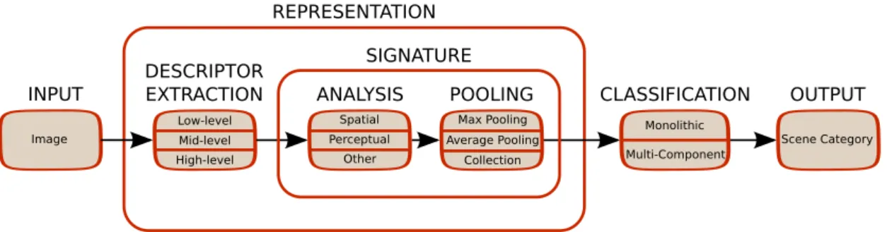
descriptors computed from the visual primitives, or it can be constructed in a statistical way, e.g. by pooling the descriptors over the full image to produce a synthetic signature. Moreover, in order to exploit the additional structure present in the considered scenes, the final representation is often constructed by performing an analysis of the spatial position of the descriptors, or of some perceptual information such as their saliency. Finally, leveraging the designed image representations, a computational model for a given scene concept (e.g. a “mountain scenery”) is constructed using one of several possible types of classifiers.
A visualization of the scene recognition pipeline considered throughout this thesis is illustrated in Figure 2.1. The proposed pipeline is only intended to be illustrative: not all the building blocks reported have to necessarily be present in a scene recognition system, while some other might be added, or might be merged together. Still, the pipeline is general enough to represent a large set of approaches that are relevant to this thesis and that will be discussed in this Chapter.
Throughout the thesis, the adjectives characterizing some parts of the representation block of the pipeline may be used to describe the overall image representation as well. For example, an image representation making use of high-level descriptors may be referred to as a high-level representation, while an image representation making use of a spatial, or a saliency analysis may be referred as a spatial representation, or a saliency-driven representation.
Before proceeding with the discussion about the different blocks of the scene recognition pipeline illustrated in Figure 2.1, it is important to dwell on how the scene recognition problem is empirically evaluated in the computer vision community. For this purpose in Section 2.1 we describe the standard datasets used for benchmarking scene recognition methods, and their corresponding evaluation protocols. The blocks of the pipeline in Figure 2.1 are extensively de-scribed in the subsequent Sections. Specifically, the descriptor extraction block, the signature block and the classification block are covered in Sections 2.2, 2.3 and 2.4, respectively.
2.1. Datasets
Table 2.1 – List of scene recognition publications and datasets used. From the list we exclude the publications in which a new dataset was proposed.
Work MIT-Indoor-67 15-Scenes Sports Other
Li et al. [2010] X X X LabelMe-9
Çakir et al. [2011] X X
Pandey and Lazebnik [2011] X
Wu and Rehg [2011] X X X
Fornoni and Caputo [2012] X X X
Kwitt et al. [2012] X X X LabelMe-9, SUN
Jiang et al. [2012] X X 21-Land-Use
Parizi et al. [2012] X
Sadeghi and Tappen [2012] X X X
Zheng et al. [2012] X X X
Juneja et al. [2013] X
Vitaladevuni et al. [2013] X X X
Fornoni and Caputo [2014] X X X
Xie et al. [2014] X SUN
2.1 Datasets
Throughout the years, three main datasets have been established as standard benchmarks for scene recognition algorithms: the MIT-Indoor-67 [Quattoni and Torralba, 2009], the 15-Scenes [Lazebnik et al., 2006] and the UIUC-Sports [Li and Fei-Fei, 2007] datasets. In Table 2.1 we report a list of recently published scene recognition approaches, with the corresponding list of scene recognition datasets used. As it is possible to see the three above mentioned datasets are used in most of the recent scene recognition publications. Accordingly, these datasets are also the main benchmarks considered in this thesis. Note that, since we focus on classification of single images, we do not consider datasets for evaluating approaches addressing the problem of classifying scenes in video sequences (e.g. [Pronobis and Caputo, 2005; Luo et al., 2006; Pronobis and Caputo, 2009; Wu et al., 2009; Pronobis et al., 2010]). In the following, for each of the three dataset considered throughout this thesis (MIT-Indoor-67, 15-Scenes and UIUC-Sports) we provide a description of the collection procedure, a description and a visualization of the images belonging to the dataset, and a description of the benchmarking procedure. In addition we provide a synthetic description of the other scene recognition datasets appearing in Table 2.1 (SUN [Xiao et al., 2010], LabelMe-9 [Li et al., 2010] and 21-Land-Use [Yang and Newsam, 2010]). For additional details we refer the interested reader to the appropriate publication.
MIT-Indoor-67
Since its introduction, the MIT-Indoor-67 dataset [Quattoni and Torralba, 2009] has become one of the most important and most challenging benchmarks for scene recognition algorithms.
bakery bookstore clothing store deli florist grocery store jewellery shop laundromat mall
shoe shop toystore
video store
Store
airport inside church
cloister
inside businside subway library museum pool inside prison cell subway trainstation waiting room locker room elevator Public place artstudio classroom computer room dental office green house hospital room kinder garden
laboratory wet
meeting room office
operating room studio music tv studio restaurant kitchen warehouse Working place
buffet fastfood concert hall
gameroom gym hair salon movie theater restaurant bowling bar casino Leisure auditorium bathroom bedroom children room closet corridor dining room garage kitchen livingroom lobby nursery pantry stairscase winecellar Home
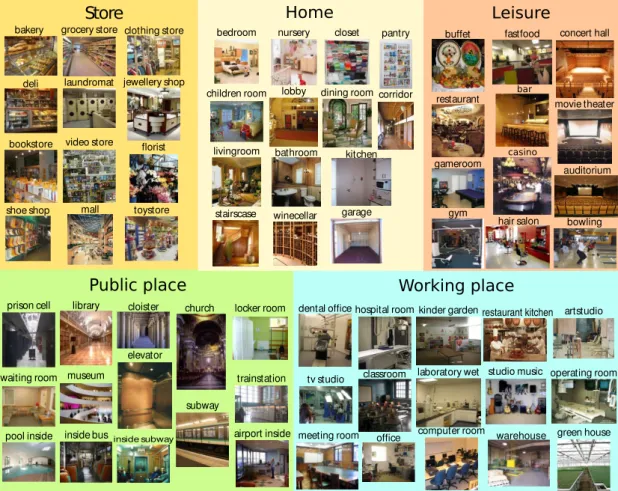
Figure 2.2 – Example images from the 67 classes of the MIT-Indoor-67 dataset, organized by scene group. (Adapted from Quattoni and Torralba [2009])
According to Table 2.1, it is now the most used dataset for this class of problems. It consists of images of indoor scenes captured in unconstrained and cluttered conditions and collected using online image search engines, online photo sharing sites and the LabelMe dataset [Russell et al., 2008]. It contains 15,620 images belonging to 67 different categories, at a minimum resolution of 200 pixels in the smallest axis and with a minimum of 100 images per category. The 67 scene categories are grouped into 5 big scene groups: Store, Home, Leisure, Public place and Working Place.
It is worth noting that in indoor environments the location of meaningful regions and objects varies drastically within each category, while the close-up distance between the camera and the subject makes the variations due to view-point changes even more severe. This results in a very high degree of intra-class visual variability. Moreover, many of the classes (e.g. classes belonging to the same scene group) present a high degree of visual inter-class similarity. Images sampled from the categories in the five scene groups are visualized in Figure 2.2. The standard benchmarking procedure for this dataset consists of randomly selecting 100 images per category and split them into 80 images for training and 20 for testing. The scene
2.1. Datasets
coast forest highway insidecity mountain
opencountry street tallbuilding industrial store
bedroom kitchen livingroom office suburb
Figure 2.3 – Example of images from the classes of the 15-Scenes dataset.
recognition performance is measured by the multiclass accuracy, defined as the average of the diagonal of the confusion matrix. Using this benchmarking procedure, the scene recognition accuracy reported at the moment this dataset was published is 26%.
15-Scenes
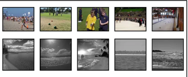
The 15-Scenes dataset [Lazebnik et al., 2006] is a well established scene recognition bench-mark, containing images of both outdoor and indoor scene environments. The collection was gradually built over the years: the initial 8 outdoor classes were collected by Oliva and Torralba [2001]; four additional indoor categories and one additional outdoor category were added by Fei-Fei and Perona [2005]; finally, two additional categories (one indoor and one outdoor) were introduced by Lazebnik et al. [2006].
In its final version, the 15-Scenes dataset contains 4485 low-resolution and gray-valued images, with 210 to 410 images per class. The 15 scene categories are: bedroom, coast, forest, highway, industrial, insidecity, kitchen, livingroom, mountain, office, opencountry, store, street, suburb and tallbuilding.
In Figure 2.3 we report one image example for each category. As it is possible to see, the inter-class similarities are lower for this dataset, with the largest visual similarities occurring amongst indoor classes.
For this dataset the standard benchmarking protocol consists in randomly selecting 100 training images per class and using the remaining ones for evaluation. The scene recognition
badminton bocce croquet polo
rock climbing rowing sailing snowboarding
Figure 2.4 – Example of images from the classes of the UIUC-Sports dataset.
performance is measured by the multiclass accuracy, defined as the average of the diagonal of the confusion matrix. Using this benchmarking procedure, the scene recognition accuracy reported at the moment this dataset was published is 81.4%.
UIUC-Sports
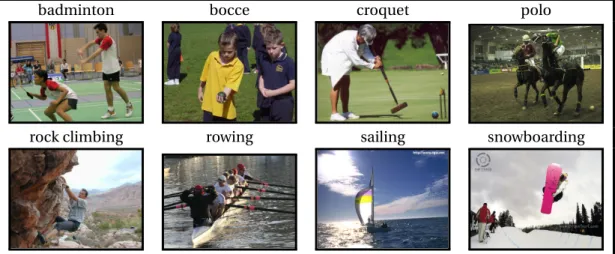
The UIUC-Sports dataset [Li and Fei-Fei, 2007] is a collection of images of sports scenes. According to the authors, although sport categories represent events and not just places (as the categories in the 15-Scenes, or the MIT-Indoor-67 datasets), sport recognition can be approximated and viewed as a scene recognition problem. As mentioned in Section 1.3, the main challenges of this problem lie in the high levels of structural variability, due to clutter and variability of the environment in which the events are taking place, and to the wide variety of subjects and poses in each category. Some sports categories, like croquet and bocce, also present high levels of visual similarity.
This dataset has been used in the large majority of works addressing scene recognition prob-lems (see Table 2.1) and it contains images from 8 sport categories: badminton, bocce, croquet, polo, rock climbing, rowing, sailing and snowboarding. The number of images per category varies between 137 and 250. A visualization of images sampled from each category is reported in Figure 2.4.
The benchmarking protocol for this dataset consists in selecting 70 images per class for the training set and 60 for the test set. The scene recognition performance is measured by the multiclass accuracy, defined as the average of the diagonal of the confusion matrix. Using this benchmarking procedure, the scene recognition accuracy reported at the moment this dataset was published is 74.4%.
2.2. Descriptor Extraction
Other datasets.
For completeness, we report here a short description of other datasets that have been occa-sionally used to evaluate the performance of scene recognition approaches:
– SUN[Xiao et al., 2010]. The SUN (Scene UNderstanding) dataset is a large scale dataset containing images from 397 scene categories, selected using the WordNet ontology [Fell-baum, 1998]. Each scene category contains at least 100 color images, retrieved using search engines. A subset of the dataset is annotated with objects.
– LabelMe-9[Li et al., 2010]. The LabelMe-9 dataset is a subset of the LabelMe dataset [Russell et al., 2008] containing images from 9 scenes categories: beach, mountain, bathroom, church, garage, office, sail, street, forest. Each class contains 100 images, split into 50 for training and 50 for testing.
– 21-Land-Use[Yang and Newsam, 2010]. The 21-Land-Use dataset contains images of aerial orthoimagery downloaded from the United States Geological Survey (USGS) National Map. There are 21 classes, each represented by 100 images.
In this Section we have provided a review of datasets, benchmarking procedures and evaluation metrics used by the scene recognition community. In the next Section we begin the discussion of the blocks composing the scene recognition pipeline introduced at the beginning of this Chapter.
2.2 Descriptor Extraction
Over time, a large number of visual primitives and descriptors have been considered for scene recognition tasks. Without aiming to be exhaustive, in this Section we will discuss the most important ones, ordering them according to the taxonomy introduced before.
2.2.1 Low-level descriptors
The descriptors belonging to this category simply consist of low-level features extracted from the visual primitives. One of the first descriptors specifically designed for scene recognition is theSpatial Envelope, also known asGIST[Oliva and Torralba, 2001]. The visual primitive considered by this descriptor is tipically either a large image patch or the full image. In this work the authors analyze the global appearance properties (not related to objects) used by humans in order to categorize outdoor scenes. By performing an experiment with seventeen human observers they argue that the five most important global properties used by humans to categorize outdoor scenes are:Degree of Naturalness, Degree of Openness, Degree of Roughness, Degree of Expansion, Degree of Ruggedness. They then propose a computational model for each of these properties and combine them to obtain a final image signature. Using this descriptor the authors obtained good results in classifying low-resolution outdoor scenes into categories like: mountains, seaside, forest, etc. All the same, the approach was later found to be unsuitable for indoor scene categories [Quattoni and Torralba, 2009].
Another example of a low-level descriptor used to address scene recognition problems is the one proposed by Linde and Lindeberg [2004]. In this work the authors suggest to use multi-dimensional histograms of low-level features (such as normalized gradient magnitude and RGB chromatic cues at multiple scales) as a robust way to describe images. The visual primitive considered by this descriptor is the full image. Exploiting the fact that multi-dimensional histograms are mostly zero except for a small portion of the cells, they design a sparse and sorted representation enabling to accumulate histograms with a number of cells of the order of 4514≈1023(14-D histogram with 45 quantization levels). The proposed descriptor obtained state of the art performances on the ETH-80 object categorization task [Leibe and Schiele, 2003], while also being successfully employed in indoor scene recognition tasks [Pronobis et al., 2010; Fornoni et al., 2010].
Local descriptors
Descriptors in this set, also referred to aslocal features, use small image patches (or regions) as visual primitives. Often, interest point detectors [Schmid et al., 2000] are used to select relevant locations in the image and extract features around them. The most influential work in this direction is arguably theScale Invariant Feature Transform (SIFT)proposed by Lowe [2004]. The visual primitives considered in this approach are image patches extracted at local extrema of the scale-space. A 128-dimensional descriptor of each patch is obtained by computing a histogram of gradient orientations (with 8 reference orientations) in each of 4×4 sub-patches. Early works have demonstrated the potential of this low-level local descriptor, with its main advantage being the robustness w.r.t. occlusion and clutter. Lowe [2004] applied it to object instance recognition in occluded scenarios, while Caputo and Jie [2009] combined it with exact and approximate matching techniques to solve object and place recognition problems. Another popular descriptor of this family is the Histogram of Oriented Gradients (HOG). Introduced by Dalal and Triggs [2005] for human detection, it has also been used for generic image classification [Bosch et al., 2007] and scene recognition [Fornoni et al., 2010] tasks. Similarly to SIFT, HOGs capture the distribution of edge orientations within a given image region (computed on the output of a Canny edge detector). The orientations range is quantized intokbins and each edge is assigned to the corresponding binned orientation, with a weight proportional to the value of the gradient. This descriptor is not rotationally invariant but has shown good performance in indoor categorization tasks [Fornoni et al., 2010], in which usually the gradient directions are not strongly rotated.
While the image representation obtained by directly using low-level descriptors have shown some initial success in image classification and scene recognition tasks, these representations may not be able to robustly describe complex scenes, like indoor ones. In order to produce robust image representations, mid-level descriptors have thus been introduced.


![Figure 3.1 – Saliency-driven segmentation of images from office and kindergarden categories (MIT-Indoor-67 dataset [Quattoni and Torralba, 2009])](https://thumb-us.123doks.com/thumbv2/123dok_us/9911078.2484298/58.892.121.742.145.389/figure-saliency-segmentation-kindergarden-categories-indoor-quattoni-torralba.webp)
![Figure 3.2 – Saliency-driven segmentation of images from badminton and snowboarding categories (UIUC-Sports dataset [Li and Fei-Fei, 2007])](https://thumb-us.123doks.com/thumbv2/123dok_us/9911078.2484298/59.892.173.769.148.355/figure-saliency-segmentation-badminton-snowboarding-categories-sports-dataset.webp)


