Stefan Tötterman
Aspects on Robust Control and
Identification
St efan Tött er man | A spec ts on R obust C ontr ol and Identification | 2019 9 7 8 9 5 2 1 2 3 8 1 0 9Aspects on Robust Control and
Identification
Stefan Tötterman
Process Control Laboratory Faculty of Science and Technology
Åbo Akademi University Åbo, Finland, 2019
ISBN 978-952-12-3810-9 (print) ISBN 978-952-12-3811-6 (pdf) Painosalama Oy
Preface
The research for this thesis was carried out during the time periods 2001 – 2009 and 2017-2019. I wish to thank my supervisor, Professor Hannu Toivonen, for his support, guidance and intelligent comments during these years. I am also grateful to the rest of the staff at the Process Control Laboratory, especially Professor Kurt-Erik Häggblom for his recent actions in pushing this project forward. Further I want to thank my co-author, Dr. Bernt Åkesson.
I am also grateful for the valuable comments on the manuscript the pre-examiners Professor John Bagterp Jørgensen and Dr. Kai Zenger provided. Furthermore I would like to express my thankfulness to my colleagues in the NAPCON business unit at Neste Engineering Solutions for contributing to a working atmosphere that encouraged me to finalize this work.
I wish to express my gratitude for financial support that I have been provided by the Finnish Graduate School in Chemical Engineering (GSCE) and Åbo Akademi University Foundation (Stiftelsen för Åbo Akademi).
Last, I want to thank my sons, Fabian and Valdemar, for having been a consistent source of joy in my life.
Åbo, April 2019 Stefan Tötterman
Abstract
This thesis treats different aspects on robust controller design and model identification techniques. The controller design technique proposes frequency-domain specifications for achieving a fixed-structure controller with user specified optimality criteria. The optimization based design method is iterative and it is based on direct shaping of the frequency responses without a need to explicitly design any weighting filters in contrast to classic loop-shaping methods. Computational efficiency has been taken into account by utilizing linear matrix equations for characterizing the frequency responses in the time-domain. The proposed controller design method can be used for designing any type of linear controllers, e.g. PID-type controllers, for identified linear systems.
Support vector regression (SVR) has several inherent excellent features that can with advantage be utilized in robust system identification. One of these is the usage of Vapnik’s -insensitive loss function that gives robustness and insensitivity to overtraining. Other features are the automatic computing of the parameters used in SVR and the convex optimization that guarantees to always find the global optimum.
SVR has in this thesis been tailored by modifying the kernel function to better fit several common model identification problems. These are identification of state-dependent parameter models or quasi-ARX models, smoothness priors models of linear systems and nonlinear Wiener models. All these proposed identification methods have been applied to examples of different systems. The results have been either as good or even better compared to other corresponding methods.
Svenskt abstrakt
Avhandingen behandlar flera aspekter kring regulatordesign och metoder för modellidentifiering. Kriterier som specificeras i frekvensplanet används för en optimal strukturbegränsad regulatordesign metod. Denna metod är iterativ och baserar sig på direkt formning av frekvensfunktioner utan att behöva formge skilda viktfilter till skillnad från klassiska krets-formgivnings metoder. Optimeringsproblemet löses med hjälp av linjära matrisekvationer som beskriver frekvenssvar direkt i tidsplanet. Regulatorsyntesmetoden kan användas för att konstruera en godtycklig linjär regulator för identifierade linjära processer, exempelvis en regulator av PID-typ.
Regression med hjälp av stödvektormaskiner (eng. support vector machines) har flera medfödda goda egenskaper som med fördel kan utnyttjas i robust system identifiering. En av dessa är utnyttjandet av Vapniks -okänsliga förlustfunktion som ger robusthet och skydd mot överträning. Andra egenskaper är automatisk beräkning av de interna parametrarna som används i stödvektormaskinerna samt att optimeringen alltid är konvex vilket garanterar att det globala optimet alltid hittas. I denna avhandling har regression med hjälp av stödvektormaskiner blivit skräddarsytt genom att anpassa strukturen på kernel funktionen så att den bättre lämpar sig för olika modellidentifieringsproblem. I avhandlingen presenteras metoder för identifiering av tillståndsberoende parametermodeller, så kallade ”smoothness priors” modeller av linjära system och olinjära Wiener modeller. Alla dessa modellidentifieringsmetoder har verifierats med hjälp av praktiska exempel på olika system och resultaten har varit lika bra eller bättre än vad andra jämförbara modellidentifieringsmetoder ger.
List of publications
This thesis consists of the following publications together with an introduction.
I. Design of fixed-structure controllers with frequency-domain
criteria: a multiobjective optimisation approach, Hannu T. Toivonen and Stefan Tötterman, IEE Proceedings – Control Theory and Applications, Vol 153, No 1, pp 46-52, 2006.
II. Smoothness priors support vector method for robust system
identification, Stefan Tötterman and Hannu T. Toivonen, IET Control Theory and Applications, Vol 3, Iss 5, pp 509-518, 2009.
III. Identification of state-dependent parameter models with
support vector regression, Hannu T. Toivonen, Stefan
Tötterman and Bernt Åkesson, International Journal of Control, Vol 80, Iss 9, pp 1454-1470, 2007.
IV. Support vector method for identification of Wiener models,
Stefan Tötterman and Hannu T. Toivonen, Journal of Process Control, Vol 19, Iss 7, pp 1174-1181, 2009.
Author’s contributions
The author of this thesis is the main author of publication II and IV and the second author of Papers I and III. The introductory part is completely produced by the author. The author has participated in both the derivations and proofs of the theoretical findings in all the papers. The author is responsible for all numerical examples and simulations appearing in all the papers. The only exception from this is Paper III, where Bernt Åkesson contributed with the feedforward neural network comparison in example 2.
Abbreviations and symbols
ARMAX Autoregressive moving average with exogenous inputs ARX Autoregressive with exogenous inputs
HF High-frequency LF Low-frequency
LQG Linear-quadratic-Gaussian LTI Linear time-invariant MF Mid-frequency
MIMO Multiple inputs, multiple outputs MISO Multiple inputs, single output
NARMAX Nonlinear autoregressive moving average with exogenous inputs RBF Radial basis function
SDP State-dependent parameter SIMO Single input, multiple outputs SISO Single input, single output SVM Support vector machine SVR Support vector regression
b Bias term
c,C Constant specified by user
d Disturbance signal
e Error signal
G Process model transfer function
Gd Disturbance transfer function H Transfer function
K Controller transfer function or kernel function
l1 Least absolute deviation
L -insensitive loss function
r Reference signal (set point)
s Laplace transform complex variable
S Sensitivity function
SC Control sensitivity function
Sl Load disturbance sensitivity function T Complementary sensitivity function
u Control signal w Weight vector x Input vector y Output signal Lagrange multiplier Lagrange multiplier Margin of -tube Basis function Slack variable
Static nonlinear system Frequency
Contents
Preface ...i
Abstract ...iii
Svenskt abstrakt ...v
List of publications ...vii
Author’s contributions ...vii
Abbreviations and symbols ...viii
Contents ...ix
1 Introduction ...1
1.1 Controller design ... 2
1.2 System identification ... 3
2 Frequency domain controller design ...6
2.1 Stability of feedback systems ... 6
2.2 Robust identification ... 8
2.3 Control performance of feedback systems ... 8
2.4 Loop shaping methods ... 10
3 Nonlinear model structures ...13
3.1 Block oriented model structures ... 14
3.1.1 Wiener models ... 14
3.1.2 Hammerstein models ... 15
3.2 State-dependent parameter models ... 16
4 Robust model identification using support vector regression ....18
4.1 Support vector regression formulation ... 19
4.2 Kernel functions ... 23
4.3 SVR as a neural network ... 24
4.4 Solving the SVR problem ... 25
4.5 Different SVR methods ... 27
5 Outline of the papers ...28
5.1 Paper I ... 28 5.2 Paper II ... 29 5.3 Paper III ... 30 5.4 Paper IV ... 31 6 Conclusions ...32 References ...34
Chapter 1
Introduction
During the last century, control engineering has systematically advanced and a common language in terms of concepts and terminology has been established. Control engineering has for decades been a standard field in engineering sciences, practically all over the world. Automatic feedback systems have indeed been used for more than 2000 years, one early example is the water clock clepsydrae which were in use in the Greece Empire by the third century BC. The Greece inventor and mathematician Ctesibius in Alexandria is considered to be a possible inventor of it [1], [2].
One of the first implementations of the PID-controller was made in 1911 by the American inventor Elmer Sperry. He implemented PID-control to automatic ship steering. In addition, compensation for disturbances was made using gain adjustment when the sea conditions changed. This was made more or less ad hoc without a complete theoretical understanding of it. The first theoretical analysis of a PID-controller was made 11 years later in 1922 by the Russian American engineer Nicolas Minorsky who also worked with research and design of automatic ship steering systems. During the 1930s the use of pneumatic controllers increased rapidly and systematic approaches to control challenges gradually started to take place. At the same time the research, advances in understanding of control system analysis and design, were made by several research groups in several countries, independently from each other. The time period 1935-1955 is often referred to as the classical period of control engineering in which many important findings were made, e.g. Nyquist and Bode diagrams as well as Ziegler-Nichols PID-controller tuning rules [1], [2], [3].
During the modern control period of automatic control, i.e. from the year 1955 onwards, several new methods and approaches were developed. The development of computers enabled more complex approaches to be used. More complex methods, such as nonlinear MPC, benefit from complex models that describe a system more accurately than simpler models. Still
today the general assumption is that more than 90 percent of all control loops are of type in the process industry [4]. Most of these PID-controllers do not utilize the derivative part and are actually implemented as PI-controllers and some even as P-controllers.
System identification has its roots in the works of the statisticians Gauss (1809) and Fisher (1912) [5]. System models were needed already during the classical period of control engineering but during the modern control period of automatic control the need for system identification grew fast. Especially in the 1960s when the development of model-based control era began with Kalman filters, pole placement, LQG control etc models that are not available from physics were needed [6], [7], [8], [9]. This resulted in the development of realization theory and the basis for subspace identification methods as well as prediction error identification methods. The era of state-space models began and since then system identification has been an essential part of control engineering. System models are also needed in other fields, e.g. environmental, biological and transportation systems, which makes system identification methods important for a wider audience.
This thesis consists of a robust controller design approach as well as different robust nonlinear model system identification approaches.
1.1 Controller design
In control theory, a controller is a device that monitors and changes the operating conditions of a dynamical system. The system may have one single input and one single output (SISO), multiple inputs and multiple outputs (MIMO), single input and multiple outputs (SIMO) or multiple inputs with a single output (MISO). Controlling a MIMO system where the interactions are found only from one input to one output is referred to as multiloop control. If the output variable in a MIMO system depends on two or more input variables we need multivariable control methods for controlling the system, e.g. decoupling control or model predictive control.
Most controller design methods are applicable on SISO systems where standard feedback controllers can be used as such. One of the simplest
types of feedback controllers are on/off controllers. When tuning this type of controllers, we do not need to know the exact dynamics of the controlled variable as long as we know in which direction the input affects the controlled variable. Obviously, the control performance cannot be very accurate using an on/off controller. To achieve higher control performance more advanced control methods are needed as well as better understanding of the systems that are controlled, i.e. accurate system models. Already for tuning a simple PI-controller an accurate model of the controlled system helps significantly in the task to find optimal controller parameters. In general, more complex controllers are needed for more complex systems to achieve satisfactory control performance.
The controller design method presented in this thesis (Paper 1) can be used in order to find optimal P, PI or PID-controller parameters and to compare the controller performance with more complex controllers, i.e. finding the optimal controller order needed and avoiding the use of a controller of unnecessary high order, on top of achieving the optimal parameters of the controller. An accurate system model is indeed needed for applying this controller design method. This is the case for almost all of the alternative methods as well. The method is presented for SISO systems but it is straightforward to extend it to at least small MIMO systems.
1.2 System identification
System identification has an essential role in process control. A mathematical model is needed to describe the dynamical behavior of the system that needs to be controlled. Based on the model an optimal controller can be designed by using different controller design methods as well as different objectives. The models can be obtained in three different manners. These are known as white box, black box and grey box modelling.
White box models are based on first principles. Mathematical models are achieved based on for example physical laws such as Newton’s equations and the laws of conservation of energy and conservation of total mass. This type of models becomes easily very complex or practically impossible to obtain due to the fact that real systems often consists of
several complex system parts that interact with each other. White box models are also referred to as first principle models.
Black box models are obtained with no prior knowledge about the dynamical behavior of the system. This type of model identification methods only looks at how the input affects the output. Numerical methods are often utilized to fit the model output to the observed measured output based on the input. A mathematical model is achieved as a result of this. The model structure, e.g. the model order of a linear system, can be assumed in advance or be derived as a part of the solution of the identification algorithm used. Black box modelling is the most commonly used model identification technique.
Grey box models are a combination of white and black box models. A part of the system dynamics is modelled using first principles and the rest of the dynamics is modeled using black box identification techniques. Fitting one or more parameters in a first principles model by using black box methods results in a grey box model. Grey box models are also referred to as semi-physical models.
Identification of nonlinear systems is a challenge since several different model structures as well as estimation approaches can be used. The choice of model structure plays an important role in identification of all kinds of models. Classical, simple first and second order linear models reveal directly information of the dynamical behavior to the user of the models, e.g. the size of gain and time constants. Also complex nonlinear system models can reveal useful information if the structure has been chosen with care. Since there are several possibilities to express complex nonlinear models it is important to choose a structure that is compatible with the dynamic behavior of the system and tells as much as possible about the dynamical behavior to the user of the model. It is easier to work with black box models that have a model structure that reveals certain information of system dynamics than to work with abstract black box models.
Another division of model identification is based on what kind of information the model uses as inputs and outputs. Prediction error identification is a common term for model identification where the model
predicts the future outputs based on past inputs and past outputs. The model identification methods that only utilize the input for describing the output are referred to as output error identification methods.
All of the identification methods described in this thesis are categorized as black box methods and the models are represented as discrete-time models. The identification method presented in Paper III is a prediction error method whilst the methods in Paper II and IV are output error identification methods. The model in Paper II is linear and the models in Papers III and IV are nonlinear. All of these models reveal something about the system dynamics directly to the qualified user. The nonlinear model structures that are used in this thesis are explained in more detail in Chapter 3.
Chapter 2
Frequency domain controller design
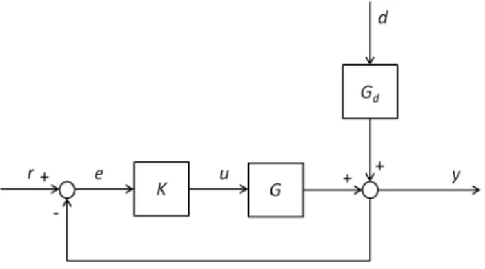
The most common way to design a control system is to take advantage of the feedback loop. A basic closed-loop feedback system is illustrated in Figure 2-1.
Figure 2-1. Closed-loop feedback system.
In the figure,G stands for the process or plant model transfer function, Gd
for the transfer function of the disturbance d and K is the controller. y is
the output signal,u is the control signal,r is the reference ande is the error signal. For simplicity, assume that all the transfer functions are SISO systems and that the system is linear.
2.1 Stability of feedback systems
Stability is an important concept in control theory. It is the most important performance criterion of a control system. There are several different definitions on stability available, e.g. [10], [11], [12] and [13]. A common definition on stability is BIBO stability where every bounded input
produces a bounded output. The closed loop output as a function ofr and
d is achieved from the block diagram above
) (r y GK d G y d (1)
d GK G r GK GK y d 1 1 (2)
The closed loop control signal dependence of r and d are also obvious
from the block diagram in Figure 2-1. )
(G d Gu
K Kr
u d (3)
Accordingly we have the closed loop transfer function fromr andd tou
d GK KG r GK K u d 1 1 (4)
According to classical system stability analysis we know that the continuous system is stable if the poles of the characteristic function have negative real values. The discrete time system is stable if all the poles have a magnitude less than 1.
The Nyquist stability criterion allows us to compute the stability based on
the open loop transfer function GK only. This is done by plotting the
complex loci of the transfer function GK for every frequency [- , ],
s = j . The simplified Nyquist criterion states that any linear feedback
system having poles with negative real values is stable if the open loop Nyquist-plot cuts the real axis to the right of point -1.
Bode plots were already in 1930s introduced as a graphical tool for determining stability of control systems. Bode plots are graphs of the frequency response of systems. More exactly Bode plots consist of both the magnitude plot and the phase plot of a system as functions of the frequency. The magnitude plot of a transfer function H(s) is thus |H(s)|
wheres = j is plotted usually on a logarithmic scale (dB) as a function of
logarithmic scaled . The phase plot is the phase, arg(H(s)), wheres = j
(degree) and it is plotted on the same logarithmic frequency scale as the magnitude plot. The stability criterion of Bode states that a linear feedback system is stable if the magnitude of the open loop transfer function is smaller than 1 (or 0 dB) for the critical frequency. The critical frequency is the frequency where the phase is -180 degrees which can directly be read from the Bode plot.
Bode plots are more widely used than Nyquist plots and they are still today a standard tool for control engineers because of their illustrative description about system dynamics. Stability and phase margins can for example easily be directly read from the plots. More details about these methods are described in almost all books describing control theory, see for instance [10], [14] and [15]. These methods lay the foundation to performance criteria and loop shaping methods.
2.2 Robust identification
Robust identification or usage of the so-called uncertain models was first introduced in the papers [16] and [17] according to [18]. This model type is identified from experimental data and can be used as the basis in robust
control. The uncertain models are described in terms ofH orl1 errors.
The usage of frequency domain robust identification procedures results in a set of models with additive dynamic uncertainty. This can directly be
used as the representation of a system that may be controlled by an H
-optimal controller. -synthesis design methods [19] can be used for this purpose.
2.3 Control performance of feedback systems
Stability is a qualification for good control performance. There are indeed several stabilizing controllers available. In order to achieve good controller performance more criteria about performance are needed. The most commonly used criteria defined in the frequency domain are the sensitivity function, complementary sensitivity function and the control sensitivity function [11], [20].
The sensitivity functionS is given by
GK S
1
1 (5)
It describes how additive disturbances (Gdd) to the process output of the
Thus it gives a practical characterization of measurement disturbance attenuation.
The complementary sensitivity function is given by
GK GK S T 1 1 (6)
and the control sensitivity function is given by
GK K KS
SC
1 (7)
The complementary sensitivity function describes the effect of a set-point
change to the output y and thus it can be used as a measure of noise
rejection. The control sensitivity function describes how output noise and
set-point changes affect the control signal u. It can be used as a
measurement of robustness for model error in G. The control sensitivity
function is also called noise sensitivity function.
Åström [11] refer to the gang of four when discussing performance criteria in the frequency domain. The gang of four consists of the three functions above expanded with the load disturbance sensitivity function
GK G GS
Sl
1 (8)
This function describes how load disturbances in the control signal transfer in the closed loop to the output. The load disturbance can be
visualized as a disturbance added to u in Figure 2-1. The load disturbance
sensitivity function is thus also called input sensitivity function. It is obvious from equations (1) – (4) from where the above mentioned functions are derived.
These functions give an understanding of the properties of a feedback system to the control designer. It is important that the transfer functions meet some specifications in certain frequency ranges. Theoretically the magnitude of all four transfer functions should be as small as possible, except the complementary sensitivity function that should be close to 1 for frequencies describing set-point changes, otherwise small, particularly for
noise frequencies. Because of the waterbed effect, or the algebraic relationships between functions (5) – (8), it is not even possible to minimize the magnitude of these functions for all frequencies at the same time. Loop shaping methods rely on giving a certain shape to the frequency responses of the performance transfer functions. This is clearly visualized by plotting the magnitude of the performance functions as a function of frequency. Traditionally loop shaping is done in a quite laborious way by iteratively and separately designing suitable weighting filters for optimization that affect the frequency responses in desired manners.
The relevant frequencies in the frequency domain are usually characterized by the closed loop bandwidth and the plant crossover frequency. The bandwidth is the frequency range beyond which the signal magnitude (gain) drops down by more than 3 dB. The bandwidth gives a measure of the speed of the transient response. If the bandwidth is large, high frequency disturbances pass easily through the system. The gain crossover frequency is the frequency where the magnitude is 1 or equivalent 0 dB. The phase crossover frequency is defined as the frequency where the phase angle is -180° [21]. In this thesis, crossover frequency refers to gain crossover frequency.
2.4 Loop shaping methods
Traditional loop shaping design methods are inherently iterative processes. To meet performance and robustness specifications, the frequency response of the closed loop transfer functions described in Section 2.3 should meet certain frequency-dependent bounds. One challenge is to find the most suitable bounds, since the trade-offs between the various frequency responses are not usually known in advance.
The most common way to shape the responses is by using H
loop-shaping methods. In order to achieve a certain shape of the response, a certain weighting filter is needed in order to form the response. Usually it is not known in advance which filter is most suitable. Because of this already the determination of the weighting filter is usually an iterative process. It is hard to know how much a change in weighting filters will
affect the closed loop responses without using trial and error. Another
shortage with traditional H loop-shaping methods is the resulting
controller achieved in the end of the iteration process described. The controller is of the same order as the generalized plant including the weighting filters. If the aim was for example to find proper PID-controller parameters this method is not well suited. The achieved high-order controller can of course be reduced to a predefined low-order controller by using model reduction methods [22], [15]. However, the controller order reduction also affects the control performance and the reduced order controller does not necessarily meet the frequency response criteria achieved with the original high-order controller.
There are several successful implementations of H loop-shaping methods
for different applications, e.g. reported in [23], [24], [25] and [26]. Typically the controller order is not important or a restricting factor in these applications. Also automatic weight selection algorithms have been presented, e.g. in [27] and [28]. These methods are quite hard to use because of a high amount of parameters that have to been set or then they are developed for a certain class of usage only. Furthermore none of these methods guarantees that the used weights are optimal.
The frequency range can be split into smaller ranges in different ways. One proposed method [20] is to split the frequency range into three smaller parts, low-frequency range, mid-frequency range and high-frequency range. Typically the mid-high-frequency range should be chosen to be an interval around the plant crossover frequency. By this division of the frequency range, it is easier to apply relevant performance measurements for the system. As proposed by [20], the relevant performance criterion in the low-frequency range is given by
2 2 ) j ( j 1 max 1 1 l l LF S S s J (9)
The performance criteria for the mid-frequency range are given by 2 2 , max (j ) 2 1 S S JMFS (10) and
2 2 , max (j ) 2 1 T T JMFT (11)
Last the criterion for the high-frequency range is given by 2 2 ) j ( max 2 C C HF S S J (12)
In the equations above, the mid-frequency interval [ 1, 2] defines the
frequency range around the crossover frequency.
The controller design method presented in Paper 1 consists of a procedure that effectively solves the multi objective optimization problem directly in the time domain without the need to define separate weighting filters. It can thus be used for direct design of a fixed structure controller of low order, e.g. a PID-controller. The procedure is iterative because the optimal shape of the performance criteria is not known in advance. A more satisfactory design is obtained in each iteration step and experience shows that it is usually enough with just a few iterations to achieve a satisfactory design. The expression of the objective cost and its derivative in this paper may not be that obvious and can thus be seen as a key result.
Dependent on the dynamical properties of the process it may be useful to introduce more frequency ranges for very complex systems in order to more easily end up with the desired shape of the performance criteria. The design method described in Paper 1 is fully supporting this. Furthermore it is straightforward to extend the method to MIMO systems where each output is considered separately. For systems with a very large number of inputs that interact with the outputs it may however be demanding for the designer to get a remarkably better design in each iteration round and to quickly find the optimal shape of the performance criteria. The proposed method is well-suited to be used by an interactive user-interface where all the design parameters can graphically be adjusted based on results from the previous iteration. The graphical user-interface should show all the performance criteria functions, their set bounds, frequency ranges and optimization criteria for the next iteration.
Chapter 3
Nonlinear model structures
Linear dynamic models are historically important since they provide a basis for many useful well-known applications such as identification, stability analysis and control synthesis. However, linear models are insufficient to be used everywhere mainly because of the poor ability to accurate enough describe strongly nonlinear behavior. The choice of model structure is very important in system identification regardless of whether it is a linear or nonlinear model.
A visual representation of a dynamical system with inputs and outputs can be realized by a block diagram. An example of this is found in Figure 2-1. The principle of superposition is applicable to all linear models. Most of the linear systems are also time invariant (LTI models), meaning that if the input sequence is shifted by a certain amount of time, the response is shifted by the same amount. Every model that is not linear is defined as nonlinear and because of this there is a wide variety of different nonlinear model structures.
One of the simplest and widely used nonlinear model classes is feedforward block oriented models. This model class is characterized by having a linear dynamic part as well as a static or memoryless nonlinear part. The linear dynamic part in feedforward block oriented models can be made of series, parallel or combinations series/parallel of different linear dynamics. The most common feedforward block oriented models are Wiener and Hammerstein models [29], [30].
A more complex model class can be derived from the same components, i.e. a linear part and a static nonlinear part, by adding feedback connection to the structure. This model class is known as feedback block oriented models. They can represent a wider range of dynamics but generally these are much harder to identify and analyze. A classic example of this model class is the Lur’e model where a control system is described to consist of a forward LTI block and a static nonlinear block that may be time-varying and has a negative feedback connection. In this thesis all nonlinear models
belong to the feedforward block oriented model class. Generally nonlinear models can roughly be divided into the following six model classes: Volterra series models, block structured models, neural network models, wavelets models, NARMAX models and state-space models [31].
3.1 Block oriented model structures
Feedforward block oriented nonlinear models such as Hammerstein and Wiener models consist of a cascade combination of a linear dynamic model and a static nonlinear function. Although the structure of these models is quite simple they have enabled approximations of many real processes from different fields with very high model accuracy.
3.1.1 Wiener models
The Wiener models are based on Volterra series representations of nonlinear dynamic systems. The Volterra series can in discrete time case be represented as [30] ... ) ( ) ( ) ( ) ( ) ( ) ( 1 2 1 1 2 1 2 1 1 1 1 0 1 2 1 M m M m M m m k u m k u ,m m h m k u m h h k y (13)
where u and y are the input and output and hk is the k:th-order Volterra
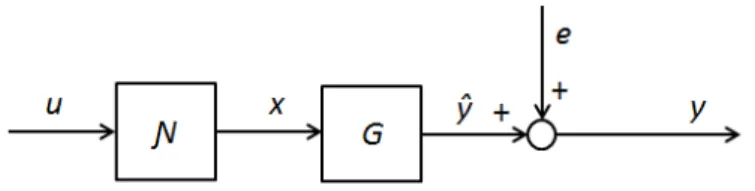
kernel. A drawback with this structure is that it typically requires a very large number of terms in order to provide high accuracy. From this starting point Wiener models were developed and are described in the book of Norbert Wiener from 1958 [32]. The model consist of a series
connection of a linear dynamic subsystemG followed by static nonlinear
Figure 3-1. Wiener model. x(n) =G(q-1)u(n)
(n) = (x(n)) (14)
y(n) = (n) +e(n)
The linear block in Figure 3-1 is not constrained to a certain structure. It can be represented by a transfer function model, Laguerre or Kautz function or other orthonormal filter expansions. Laguerre and Kautz basis have been used in many successful system identifications. As a rule of thumb, Laguerre basis expansions are preferred for well-damped dynamical systems and Kautz basis expansions are suitable for identification of dynamical systems with second order resonant modes.
Also the nonlinear block can be represented by different structures such
as polynomial expansions, radial basis functions and multilayer perceptrons.
It has been shown in [33] that Wiener models can approximate any nonlinear system with high accuracy under mild continuity conditions. The Wiener model structure has successfully been used for a great variety of different processes such as pH processes, processes with sensor nonlinearities, fluid flow systems, separation processes, fluid catalytic cracker units etc.
3.1.2 Hammerstein models
The Hammerstein model is the reverse combination of the blocks in the Wiener model as illustrated in Figure 3-2 below.
Figure 3-2. Hammerstein model.
Hammerstein models were already in 1966 suggested to be used for identification by Narendra and Gallman [34]. Examples of processes that have been successfully identified by the Hammerstein model structure are pH neutralization, spark ignition engine torque, continuous stirred tank reactors and fuel cells [35]. A discussion on dynamical differences between Wiener and Hammerstein models can be found in [36]. A combination model consisting of a static nonlinear block in the middle between two linear blocks is known as a Wiener-Hammerstein model.
3.2 State-dependent parameter models
State-dependent parameter models (SDP) are useful for modelling nonlinear systems where the model parameters are functions of the system states [37]. In this thesis, SDP models are defined as models whose parameters are nonlinear functions of past inputs and outputs. In mid 1980s Leontaritis and Billings introduced nonlinear ARMAX models (autoregressive moving average models with exogenous inputs), where the output of the nonlinear system is a function of past inputs, outputs and prediction errors [38]. Models having a nominal linear structure with state-dependent parameters are useful since they provide an insight to the model dynamics.
One common type of these models is called state-dependent ARX models or quasi-ARX models [39], [40]. In these models the linear structure follows the ARX structure but the parameters are nonlinear functions of past inputs and outputs.
) ( ) ( ... ) 1 ( ) ( ) ( ) ( ... ) 1 ( ) ( ) ( 1 1 b n a n n k u k b k u k b n k y k a k y k a k y b a (15) wherev(k) is a vector of past outputs and inputs.
) ( ... ) 2 ( ) 1 ( ) ( ... ) 2 ( ) 1 ( ) ( u y n k u, , k u , k ,u n k ,y , k ,y k y k (16) In these models the user can directly obtain locally valid linear models with visible dynamic properties and they may be treated as linear models whose parameters are taken as functions of scheduling variables. Quasi-ARX models can also be extended to quasi-ARMAX models in a straightforward way. The quasi-ARMAX model structure has turned out to be useful for modelling stochastic systems [39].
Chapter 4
Robust model identification using support vector
regression
Support vector machines (SVM) are tools for nonlinear classification and regression. Support vector machines are built on statistical learning theories and were originally developed to solve classification problems. Support vector regression (SVR) has been proven to be both a powerful and a robust tool for model identification. The present form of SVR was introduced by Vladimir Vapnik and his co-workers at AT&T Bell Laboratories in the mid 1990s [41]. Soon after their introduction SVMs have become a standard toolbox for machine learning. SVMs for both classification and regression have been applied successfully to different demanding tasks [42], [43], [44], [45], [46]. They have also performed significantly better than more traditional modelling methods in a number of different regression tasks [47], [48], [49], [50], [51].
All the model identification methods in this thesis, i.e. Paper II, III and IV, utilize SVR. The basic principle of SVR is thus presented in this chapter. More detailed information about SVR can for example be found in [52], [53], [41], [54].
The basic idea in SVR is the same as in neural network approximations. The identification is done on the basis of some input – output data. During the identification or regression, also known as the training phase, the SVR sorts out redundant information from the input data and saves the non-redundant data. After the training, the relevant information is used to build up the approximating function. The memorized model is often used to simulate an output of another input sequence of the same system, i.e. predict the output. When the predicted output is compared to the known real output the model is evaluated and this is called the validation phase.
4.1 Support vector regression formulation
In this section the classical SVR problem, the so-called -SVR, is
formulated. The task is to find an accurate estimation of a given output y
on the basis of some input vectors x={ } where each vector element
defines a different input signal. Suppose there is a set of training data
{ , } of length N and a set of basis functions { ( )} . The basis functions are often nonlinear functions that map the input data to a higher
dimension called feature space. The estimation yest of the output y is
linearly expanded in terms of nonlinear basis functions,
b b w y N T i i i est x w x 1 (17)
wherew is a weight vector andb is a bias term. In -SVR, an -insensitive
loss functionL is minimized during the training phase,
est est est est y y y y y y y y L if 0 if , , , (18)
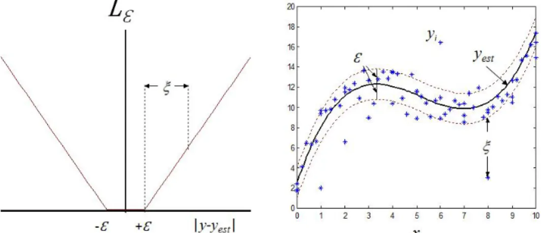
The cost L is insensitive to errors smaller than and is affected by errors
which are greater than . The cost L for the one-dimensional regression
case is illustrated in the left part of Figure 4-1 below. The space where |y-yest|< is often and as well in this thesis referred to as the -tube. In the
right part of Figure 4-1 the -tube is illustrated as a function of the input
data around the estimated functionyest.
Figure 4-1. The -insensitive loss function as a function of the regression error (left). The -tube is illustrated between the dashed lines in a regression problem (right).
The norm of the weight vector w is also minimized for flatness reasons. This enhances robustness. The minimization problem takes the form,
N i i est,i C' y y L N 1 2 ) ( 1 min , w (19)
where C' is a constant weight. The L criterion in the above optimization
objective is reformulated by introducing two sets of nonnegative slack
variables, N i i 1 and N i i
' 1. The L criterion can then be written as a
constraint, N i ' y b b y i i i T i i T i 1,2,..., ) ( ) ( x w x w (20)
and the cost function to be minimized is given by
w w w N T i i i i i ' C ' b R 2 1 ) ( 1 , , , (21)
In order to end up with the standard SVR problem for regression, the
Lagrangian functionJ of this optimization problem is introduced,
N i i i i i N i i i T i i N i i i i T i T N i i i ' ' ' b y ' y b ' C ' ' ' b J 1 1 1 1 ) ( ) ( 2 1 x w x w w w w, , , , , , , (22)
where i, 'i, i and 'i are nonnegative Lagrange multipliers. The
Lagrangian function should be minimized with respect tow,b, i and 'i.
The Lagrangian function should be maximized with respect to i, 'i, i
it is a nonconvex problem. The optimum is found by forcing the partial derivatives of the Lagrangian function to be zero, i.e.
0 i i ' J J b J J w (23)
and maximizing the resulting function. This follows from the saddle point condition for optimality. By forcing the partial derivatives to zero one gets the following conditions:
) ( 1 i N i i i ' x w 0 1 N i i i ' i i C (24) i i C ' '
The first condition in (24) follows from requiring the partial derivative
with respect to w to be zero. The second condition in (24) follows from
requiring the partial derivative with respect to b to be zero. The two last
conditions in (24) follow from forcing the partial derivatives with respect
to i and 'i to be zero. Substituting these equations (24) into the
Lagrange function (22) and after getting rid of constant terms the cost Q is
achieved which is only dependent on the iLagrange multipliers,
N i j i j i T j j N j i i N i i i N i i i i K ' ' ' ' y ' Q 1 1 1 1 ) ( ) ( ) ( 2 1 , x x x x , (25)
This function is convex, i.e. the global optimum of this function is always found. By using the cost (25), the dual problem for support vector regression can be written as
N i j i j j N j i i N i i i N i i i i ' K ' ' ' ' y 1 1 1 1 , ) ( 2 1 max x x , (26) subject to C ' C ' i i N i i i 0 0 0 1 i=1,2,...,N (27)
By substituting the uppermost condition in (24) into (17) the approximating function is given by
b K ' y N i i i i est 1 ) ( ) ( x ,x (28)
Remark 1: The quadratic term T(xi) (xj) has been written as K(x
i,xj).
This is the inner-product kernel for the SVR problem. The input data and basis functions only appear in the kernel function in the optimization setup. Because of this, there is no need to explicitly compute the basis functions at all. It is enough to directly compute the kernel values. Noteworthy is also that the number of basis functions in (17) may be infinite and it still turns out that it is for optimality enough to only
compute the kernel values of dimensionN×N. This is often referred to as
the kernel trick [55], [56], [57].
Remark 2: Most of the terms or factors( i 'i)in the equations above
that correspond to each input vector will be zero after the training. The nonzero terms correspond graphically to observations that lie outside the -tube. They also define the support vectors which are then sorted out and used for constructing the estimating function. Obviously, the name support vector machine originates from this.
4.2 Kernel functions
The kernel functions are very important in support vector machines. The basis functions are often nonlinear. Nonlinear kernel functions map the input data to a higher space called feature space and computes an inner-product there. The idea is a classical result from 1960s that enables the curse of dimensionality to be addressed [58], [59]. As was mentioned earlier, there is no need to compute the basis functions separately. Instead,
the kernel values are computed directly on the basis of the input data x.
One cannot however use an arbitrary function as a kernel function. The requirement is that they have to satisfy Mercer’s theorem from the year 1909. The theorem characterizes a symmetric positive inner-product kernel. It is a continuous analog of the singular-value (or eigenvalue) decomposition of a symmetric positive definite matrix. Details can for example be found in [52], [41] and [60]. The most commonly used kernel function in SVR is the radial basis function,
2 0 ) ( c i j j i, e K x x x x (29)
Example of other functions that satisfy Mercer’s theorem and have been used as kernels are polynomial,
1 ) ( ) ( 0 c j T i j i, c K x x x x (30)
two layer perceptron or sigmoids,
) tanh( ) ( , c0 c1 K T j i j i x x x x (31)
Fourier series, splines, B -splines etc.
Moreover, all linear combinations of permissible kernels with positive coefficients form new allowed kernels (the kernels have to be positive definite). One can also form new kernels via the tensor product of existing
kernels. In the kernels presented above, the constants c0 and c1 are
4.3 SVR as a neural network
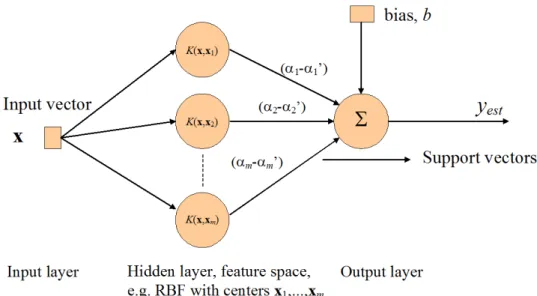
SVR can be interpreted as a neural network with one hidden layer. The architecture of SVR is illustrated in Figure 4-2.
Figure 4-2. Architecture of support vector machine for regression.
The SVR can be seen as a feed-forward neural network consisting of one
hidden layer. If the input data has N data samples, the input layer consist
of the input data vectorsx= x1,x2, ...xN where the element vectors in turn
consist of different input signals at the same time, i.e. number of different input signals. The kernels are placed in the hidden layer. During training
there is one kernel node for each input vector (N =m). The kernel values
have to be computed between each training data sample. The factors ( i - i’) are seen as weights from the feature space to the output space.
Most of the weights are zero after successful network training. The nonzero weights define the support vectors which determine which part of the data is not redundant and should be stored. The stored data can then be utilized for computing new kernel values between the support vectors and a new unseen data input, resulting in a prediction of the output.
The support vector network is highly automated. All the important network parameters are computed automatically. If radial-basis function (RBF) kernels are used, resulting in a radial basis network, the number of kernels is determined by SVR. Also their centers, linear weights and bias levels are determined by the method automatically.
4.4 Solving the SVR problem
In the previous chapter it was stated that most of the network parameters are computed automatically by the method itself. However, some parameters have to be fixed by the user. Earlier it was mentioned that depending on which kind of kernel one wants to use, one or more kernel-parameters have to be fixed by the user. Also the margin of the -tube
and the C weight that penalizes the residuals outside the -tube have to be
determined by the user. The rest of the network parameters are automatically computed in contrast to ordinary neural network where the structure of the network has to be separately specified by the user.
There may also be a need to elucidate the number of optimization variables and memory requirement when carrying out the regression task described in Chapter 4.1. As can be seen there are two optimization
variables iand ' for each input data vector. These variables are indeedi
very closely related to each other and the actual number of variables in principle equals the length of the training samples. More demanding is the memory requirement. The memory requirement is proportional to the square of the length of the training samples. The kernel values have to be computed and memorized between every input training sample.
To get an understanding of how demanding the optimization problem is the following simple example is considered: let the training data consist of
three input sequences of length N=100. The number of optimization
variables is about 100 depending on which method is chosen to carry out the optimization. The kernel values have to be calculated and memorized between every input data vector, that is 100 100 = 10 000 values. These
values are symmetric because the value for xaandxb is the same as forxb
and xa whena b, resulting in that the actual need is 5050. One can notice
numbers. They only affect the length of the input vectors (here the length is 3) which in turn has a small effect on the kernel computations.
The optimization problem is equivalent to solving a quadratic optimization (QP) problem with constraints defined below.
x c x x x T TQ 2 1 min (32) Subject to b x A (33)
The constraint means that every entry of vector Ax is less than or equal to
the corresponding entry of vectorb.
There exist a number of different efficient techniques to solve the QP problem and they will not be considered here. The most common way to solve the QP problem is by decomposition of the original dual problem. The decomposition method is also called chunking or working set method. More detailed information about this can for example be found in [41], [54] and [61].
The LIBSVM software package [62] has been used to solve the SVR problems in the Papers II-IV. The software is freely available and detailed information about the algorithms implemented can be found in [63]. It also solves the QP problem by decomposition of the dual problem.
Nowadays there is a lot of different software available for solving SVM optimization problems. See for example [64] for a list with more than 40 different available software packages. Explicitly may be noticed that there is an SVR application included in the Statistics and Machine learning Toolbox of Matlab [65]. A computationally more powerful implementation of SVR than LIBSVM is CVX, a package for solving convex optimization problems [66], at least compared to the old versions of LIBSVM from the year 2001.
4.5 Different SVR methods
Variants of the standard SVR method presented in this chapter can be achieved by substituting the -insensitive loss function with another loss function. Some examples on other loss functions that can be used are polynomial, Gaussian and Laplacian.
Separately can be mentioned least squares SVR or LS-SVR. This is a reformulation of the standard SVR problem. In this method the sum of the squared residuals are directly minimized in the cost function instead of the -insensitive loss function. The optimality conditions lead to a set of linear equations and thus LS-SVR is not a QP problem as classical support vector machines are and solving the optimization problem is simpler. The SVR model achieved is indeed more complex since the whole training data set is used as support vectors.
The size of in the -tube correlates with the number of support vectors needed. Instead of fixing the -margin the number of support vectors can be fixed and the -margin can be a variable determined by the method. This variant of SVR is called -SVR and the training phase differs in how the problem is parametrized. A detailed description of this method can be found for example in [61].
Chapter 5
Outline of the papers
5.1 Paper IDesign of fixed-structure controllers with frequency-domain criteria: a multiobjective optimisation approach
An iterative design of fixed-structure controllers, e.g. PID-controllers, with frequency-domain criteria is presented. An interactive and multiobjective optimization procedure is presented that directly shapes the frequency responses such as for example the sensitivity function and the complementary sensitivity function. In each iteration stage, a constrained optimization problem is formulated in such a way that successive improvements of the design are achieved according to the designer’s specifications. In this method there is no need to specify any weighting filters explicitly.
The frequency-domain costs are formulated in terms of state-space expressions defined in the time domain. The expressions consist of linear matrix equations and the calculations are based on real-valued arithmetics which are solved using powerful numerical optimization techniques. The computations are similar to the computations used to solve matrix Lyapunov equations in linear quadratic control.
Two numerical examples are presented in order to demonstrate the iterative design procedure. In the examples it is shown that only a few iterations are needed in order to find a satisfactory design. Since there is no need to iteratively design any weighting filters for the frequency responses at all, this method is more straight-forward and simpler than traditional methods.
5.2 Paper II
Smoothness priors support vector method for robust system identification
In this paper, linear dynamical systems are identified by an output error identification method that utilizes SVR. The system transfer function is expanded by a class of orthonormal filters, such as Laguerre or Kautz filters. An apparent advantage using SVR is the robust performance to new data achieved by using Vapniks -insensitive loss function in addition to a regularization term that increases the smoothness of the identified model.
The method proposed in the paper introduces an additional weight to the regularization term that further improves the smoothness. The weighted regularization term defines a frequency-domain smoothness prior. This
smoothness prior equals the square of the L2-norm of the m:th order
derivative of the frequency response function of the model and has thus an practical and easy understandable impact as a smoothness prior. Because of the regularization, the identified model complexity is reduced and thus the model can be more accurately approximated by a low-order model. This is an important feature since models based on basis function expansions inherently tend to have high model order. In case the identified model is an accurate representation of the system, it is possible to also obtain accurate low-order models by using standard model reduction techniques.
In the paper it is shown that this method can be implemented in a straightforward way using standard SVR with a kernel function of a specific structure. Two examples demonstrate the identification method and show that accurate low-order models can be obtained.
5.3 Paper III
Identification of state-dependent parameter models with support vector regression
State-dependent parameter models can exactly represent a broad class of nonlinear sampled-data systems. A support vector regression method is presented for identification of this kind of models. State-dependent parameter ARX models or quasi-ARX models can be identified from available input-output data by function approximators to describe the model parameters as functions of past inputs and outputs. By using this model structure and requiring a certain model accuracy, it is possible to achieve a model with fewer parameters than by using a general black-box model. This is a prediction error identification method.
Generally, support vector machines are well-suited for regression tasks since the regression cost is based on Vapniks -insensitive loss function. It has robust performance to new data and the optimal model complexity is automatically determined. On top of this, a unique and globally optimal solution is always guaranteed.
It is shown in the paper that the problem to identify quasi-ARX models reduces to a standard support vector regression problem with a modified kernel function. The modified kernel function consists of a sum of different kernels that represent individual model parameters. Results of numerical examples show that quasi-ARX support vector models give accurate parameter estimates for system that have state-dependent parameter representation. Compared to standard SVR model, quasi-ARX SVR models have higher model accuracy and are built on a smaller number of support vectors.
5.4 Paper IV
Support vector method for identification of Wiener models
Support vector regression is applied to identify nonlinear systems described by Wiener models. The linear component of the model is represented by a basis filter expansion and the static nonlinear block is represented by kernel functions. The modelling method is an output error identification method where the model output is a function of the system input only and does not depend on measured system outputs.
Support vector regression is well suited for this model identification task. Convergence to global optimum is always guaranteed and robust performance to new data is obtained through the use of Vapniks -insensitive loss function. A drawback with this method is the model complexity. Typically quite a large number of support vectors are needed resulting in a complex model.
It is demonstrated in the paper that this procedure gives accurate models of systems which have a Wiener model structure. The method was applied to a benchmark problem and the achieved accuracy based on the output error is similar compared to other output error methods where the same benchmark problem has been used.
Chapter 6
Conclusions
Since most of the controllers in the process industry are of PID-type, it is still today important to develop user friendly tuning methods for fixed structure linear controllers. Frequency loop shaping methods are inherently iterative procedures. In Paper I, a new approach for designing a fixed-structure linear controller is presented that is more straightforward to use compared to traditional methods. By using this method the designer does not need to specify any weight filters and a more satisfactory design is achieved in every iteration step. In order to productify this method, a fancy user interface can be developed by quite a small effort that can visualize all the interactive design parameters existing in this method as well as contemporary iteration results of controllers with different structures. It would further improve and clarify the iteration results to the designer. A drawback with this tuning method is that it can only be used offline and needs a model of the system to be tuned as an input.
Another area in this thesis is model identification using support vector machines for regression. Paper II, III and IV all utilizes SVR in different manners. The inherited nice features of SVR are the convergence to global optimum and robustness to new data that originates from the use of Vapniks -insensitive loss function. These features are also directly utilized by the proposed identification methods. One challenge in model identification based on measured data from a real process system is the quality of the data. In principle, all measured data are inexact. This is for example due to measurement errors and noise. Another aspect of the data quality is the state or generality that the data represent. It is therefore important that the identification or training data excites the system in all directions for which the model will be used. The SVR method is well-suited to capture relevant dynamics when the training data represents all interactions that are supposed to be included in the identified model. In Papers II-IV, it is shown that standard SVR can be tailor made for different regression purposes by only manipulating the kernel function of SVR. Several other modified SVR methods exist as well, e.g. [67] and
[47]. There are certainly more potential applications of modified SVR to be used for different model structures. This is thus an area for research in the future as well.
Even if the research on more efficient methods for solving SVR problems has proceeded it is however quite time consuming to solve an SVR problem, especially when the training datasets are large. This may limit some SVR methods to be used as online applications. On the other hand, several online applications of SVR have been reported and the computational resources in computers tend to increase all the time.
References
[1] S. Bennett, "A brief history of automatic control",IEEE Control Systems,pp. 17-25, 1996.
[2] S. Bennett, "A history of control engineering 1800-1930",IEEE
Control Engineering Series 8,1986.
[3] N. Minorsky, "Directional stability of automatically steered bodies",
Journal of the American Society for Naval Engineers, vol. 34, no. 2, pp. 280-309, 1922.
[4] K. J. Åström and T. Hägglund, Advanced PID Control, Lund
University, ISA - Instrumentation, Systems and Automation Society, 2006.
[5] M. Deitler, "System identification and time series analysis: Past,
present and future", inStochastic Theory and Control, Kansas USA,
2002, pp. 97-108.
[6] R. Kalman, "Contributions to the theory of optimal control",Boletin de la Sociedad Matematica Mexicana,no. 5, pp. 102-119, 1960. [7] R. Kalman, ”A new approach to linear filtering and prediction
problems”,Transactions ASME,nro 82, pp. 34-45, 1960.
[8] B. Ho and R. Kalman, "Effective construction of linear state-variable
models from input/output functions",Regelungstechnik, Vol. 14, pp.
545-548, 1965.
[9] K. Åström and T. Bohlin, "Numerical identification of linear dynamic
systems from normal operating records", inProc. IFAC Symposium
on Self-Adaptive Systems, Teddington, UK, 1965. [10] K. J. Åström, Reglerteori, Almqvist & Wiksell, 1968.
[11] K. J. Åström and R. M. Murray, Feedback Systems, Princeton University Press, 2008.
[12] M. Gopal, Modern control system theory, New Age International, 1993.
[13] Z. Gajic and M. Lelic, Modern control systems engineering, Prentice Hall, 1996.
[14] U. Bakshi and V. Bakshi, Control system engineering, Technical Publications Pune, 2008.
[15] S. Skogestad, Multivariable feedback control, Wiley, 1996. [16] G. Gu, P. Khargonekar and F. Lee, "Approximation of
infinitedimensional systems",IEEE Transactions of Automatic
Control,no. 34, pp. 610-618, 1989.
[17] A. Helmicki, C. Jacobson and C. Nett, "Control oriented system identification: A worstcase/deterministic approach in H-infinity",
IEEE Transactions on Automatic Control,no. 36, pp. 1163-1176, 1991.
[18] M. Mazzaro, P. Parillo and R. Sánchez Peña, "Robust identification toolbox", Latin American applied research, 2004.
[19] K. Zhou, J. Doyle and G. K., Robust and Optimal Control, Prentice-Hall, 1996.
[20] B. Lennartson and B. Kristiansson, "Pass band and high frequency
robustness for PID control", inProceedings of the 36th conference on
Decision & Control, San Diego, California, 1997.
[21] W. Zhang, Quantitative process control theory, Automation and control engineering series, CRC Press, 2012.
[22] D. McFarlane and K. Glover, Robust controller design using normalized coprime factor plant descriptions, Springer, 1990.
[23] A. Davidson and S. Ushakumari, "H-Infinity Loop-Shaping Controller for Load Frequency Control of a Deregulated Power
System",Procedia Technology,vol. 25, pp. 775-784, 2016.
[24] K. Tsakalis, S. Dash, A. Green and W. MacArthur, "Loop-shaping controller design from input-output data: application to a paper
machine simulator", IEEE Transactions on Control Systems
Technology, vol. 10, no. 1, pp. 127-136, 2002.
[25] F. Boeren, R. van Herpen, T. Oomen, M. van de Wal and O. Bosgra, "Enhancing performance through multivariable weighting function design in H-infinity loop-shaping: With application to a motion
system", inAmerican Control Conferense, Washington, DC, USA,
2013.
[26] A. Sebastian and S. Salapaka, "H-infinity loop shaping design for
nano-positioning", inProceeding of the American Control
Conference, Denver, Colorado, USA, 2003.
[27] S. Sarath, "Automatic Weight Selection Algorithm for Designing H
Infinity controller for Active Magnetic Bearing",International
Journal of Engineering Science and Technology,vol. 3, no. 1, pp. 122-138, 2011.
[28] A. Abdoljalil and E. Abolfazl, "Optimal Design of Robust Controller for Active Car Suspension System Using Bee’s Algorithm",
Computational research progress in applied science & engineering,
vol. 02, no. 1, pp. 23-27, 2016.
[29] R. Pearson, Discrete-Time Dynamic Models, Oxford University Press, 1999, pp. 87-109.
[30] F. Giri and E. Bai (editors), Block-oriented Nonlinear System Identification, volume 404 of Lecture notes in Control and Information Sciences, Springer, 2010.