Vol. 8, No. 2, June 2020, pp.1115-1130
Bayesian estimation and variables selection for binary composite quantile
regression
Taha Alshaybawee, Ahmad Naeem Flaih, Fadel Hamid Hadi Alhusseini
Department of Statistics, College of Administration and Economics, University of Al-Qadisiyah
ABSTRACT
In this paper, Bayesian hierarchical model proposed to estimate the coefficients of the composite quantile regression model when the response variable is binary. For selecting variables in binary composite quantile regression lasso the adaptive lasso penalty is derived in a Bayesian framework. Simulation study and real data examples are used to examine the performance of the proposed methods compared to the other existing methods. We conclude that the proposed method is comparable.
Keywords: Bayesian regression, Composite quantile regression, Adoptive lasso, Prior distribution, Variable selection.
Corresponding Author: Taha Alshaybawee
Department of Statistics, College of Administration and Economics, University of Al-Qadisiyah, Al Diwaniyah, Iraq
E-mail: [email protected]
1. Introduction
Modelling the relationship between the average of a dependent variable Y with the set of explanatory variables X not always be convenient. In many application studies mean regression may be not appropriate to describe the behavior of outcome variable Y with covariates variable X. For example, the effect of demographic properties and maternal conduct on the weight of infant born was study by [1] in the United States. This study concerned in low birth weight for infant it is cause many health problems, these data analyze by standard mean regression, the conditional mean was not attractive approach for low tail distribution. Quantile regression (QReg) was proposed by [14] as an extension for standard mean regression to conditional different quantiles of a dependent variables. Quantile regression model is a capable of providing a complete information about different quantiles of the stochastic relationships between dependent and predictors variables. Recently, quantile regression has received much attention in theoretical and application study, it is applied in different field of study biology, medicine, survival analysis, financial and economics and environment for more detail see [26].
For any 𝜏th quantile, (0 < 𝜏 < 1) , the 𝜏th quantile regression can be denoted as 𝑄𝑦𝑖|𝑥𝑖(𝜏) = 𝑥′𝑖𝛽𝜏 , where 𝑦𝑖 is the response variable, 𝑥′𝑖 is a k-dimensional vector, 𝛽𝜏 is a coefficient vector of quantile regression. To estimate the coefficient vector [14] proposed this equation
∑ 𝑛
𝑖=1
where 𝜌𝜏(𝑢) = 𝜏(1 − 𝐼(𝑢 < 0)), 𝐼(𝑢 < 0) is the indicator function this equation can be minimization by the algorithm proposed by [13]? Bayesian method employ to estimate quantile regression coefficient where the errors are independent asymmetric Laplace distribution [25].
In recent years, selection important subset of explanatory variables takes a lot of attention in the literature, many techniques suggest to get the important groups in the model for instance, lasso [24], SCAD [8], the elastic net method [29], adaptive Lasso [28]. Variables selection techniques has been used in quantile regression model, lasso penalty was applied to the mixed-effect QReg model or longitudinal data by [12], a solution path was introduced by [19] to 𝐿1-penalized for quantile regression model. Bayesian hierarchical model was proposed by [18], in lasso, group lasso and elastic net in quantile regression. In linear-mixed quantile regression A hierarchical Bayesian Lasso was used by [2] and was developed Bayesian adoptive lasso in quantile regression [3].
Binary quantile regression was developed for by [20,21], he was employed quantile regression in a classification and indicted to the drawbacks in the frequentist process as the difficulty optimization to estimate the parameters and the problem of computing confidence interval to the parameters. [16] studied models with binary response variable by quantile regression and was concluded this approach drive to good classification. Bayesian approach was adopted by [5] to avoid the drawback that mention above by setting some assumptions on the error term. [22] considered approach that proposed by [6] to evaluate the credit risk was modelled by binary quantile regression. New method was proposed for estimating the coefficients in regression model called composite quantile regression (CQReg), and show the relative efficiency of these estimators is greater than 70% when compare with least square estimator regardless of the error distribution [30]. Composite quantile regression (CQReg) estimators are robust to the heavy tailed or outliers in the dependent variables and more efficient than a single quantile regression. For these characteristics we employ this approach in this study.
The novel in this paper, Bayesian hierarchical model proposed to estimate the coefficients of the composite quantile regression model when the response variable is binary. For selecting variables in binary composite quantile regression lasso and the adoptive lasso penalty is derived in a Bayesian framework.
2. Prior assumptions and hierarchical models
2.1. Bayesian Binary composite quantile regression model (BBCQReg) Consider the following model
𝑦 𝑖 = 𝑏𝜏+ 𝑥𝑖′𝛽 + 𝜀𝑖, 𝑖 = 1, … … . , 𝑛 , 𝑦𝑖 = ℎ(𝑦 𝑖) (2) 𝑦𝑖 = {1 𝑖𝑓 𝑦 𝑖 ≥ 0 0 𝑖𝑓 𝑦 𝑖 < 0
Where 𝑦𝑖 is an observed binary response variable determined by the unobserved scalar latent variable 𝑦 𝑖 , 𝑏𝜏 is the 𝜏𝑡ℎ quantile intercept parameter where 0 < 𝜏 < 1, 𝑥𝑖′ is a p-dimensional vector of explanatory variables, 𝛽 is a vector of coefficient, 𝜀𝑖 is the error term. For (0 < 𝜏1 < 𝜏2< ⋯ < 𝜏𝑞 < 1), composite quantile regression parameters estimate by solving the following equation
(𝑏̂𝜏1, 𝑏̂𝜏2, … … , 𝑏̂𝜏𝑞, 𝛽̂) = 𝑎𝑟𝑔 ∑ 𝑞 𝑗=1 {∑ 𝑛 𝑖=1 𝜌𝜏𝑗(𝑦 𝑖− 𝑏𝜏𝑗− 𝑥𝑖 ′𝛽)} , (3)
where 𝜌𝜏𝑗(𝑡) = 𝑡 (𝜏𝑗− 𝐼(𝑡 < 0)), is the check function and 𝐼(. ), is indicator function, 𝜏𝑗= 𝑗
𝑞+1 , 𝑗 = 1,2, … . . , 𝑞. Equation (3) is a mixture of the objective functions from different quantile models.
Quantile regression was adopting by many researchers to treatment the models with binary response variable see for example [20,21,16,9,5,6]. Recently, composite quantile regression (CQReg) that proposed by [30] have been proven more efficient than the single quantile regression and more robust in the non-normal distribution for the error. To ameliorate the efficiency of CQReg a new estimation approach was proposed by [27], based on different weights of the components and they introduced a technique to estimate the optimal weight. Follow [27], weighted composite quantile regression proposed in this paper to model the binary response data, so Equation (3) rewrites as follow: (𝑏̂𝜏1, 𝑏̂𝜏2, … … , 𝑏̂𝜏𝑞, 𝛽̂) = 𝑎𝑟𝑔 ∑ 𝑞 𝑗=1 {∑ 𝑛 𝑖=1 𝑤𝑗𝜌𝜏𝑗(𝑦 𝑖− 𝑏𝜏𝑗− 𝑥𝑖′𝛽)} (4) where the weight 0 ≤ 𝑤𝑗 ≤ 1, and ∑𝑞𝑗=1 𝑤𝑗 = 1, for each component 𝑗𝑡ℎ.
The latent variables 𝑦 1, 𝑦 2, … … , 𝑦 𝑛, come from an asymmetric Laplace distribution with parameters 𝐴𝐿𝐷(𝜇 = 𝑏𝜏+ 𝑥𝑖′𝛽, 𝜎 = 1, 𝜏), for identification reasons 𝜎 set at unity, for more detail, see ([5, 15, 25]),
𝑝(𝑦 𝑖|𝑦𝑖, 𝑥𝑖, 𝑏𝜏, 𝛽, 𝜏) = 𝜏(1 − 𝜏)𝑒𝑥𝑝 (−𝜌𝜏(𝑦 𝑖− 𝑏𝜏− 𝑥𝑖′𝛽)). So the joint distribution function of 𝑦 = (𝑦 1, 𝑦 2, … … , 𝑦 𝑛) given 𝑋 = (𝑥1′, 𝑥2′, … … , 𝑥𝑛′)′is:
𝑙 = ∏𝑞𝑗=1 ∏𝑛𝑖=1 𝜏(1 − 𝜏) 𝑒𝑥𝑝 𝑒𝑥𝑝 (− 𝑤𝑗𝜌𝜏𝑗(𝑦̌𝑖− 𝑏𝜏𝑗− 𝑥𝑖′𝛽)) (5)
Maximization the likelihood function (5) is equivalent to Minimization the loss function (3), Equation (5) is difficult to solve directly, follow f [10] cluster assignment matrix 𝐾 with the elements
𝑘𝑖𝑗= {
1 when ith belong to jth cluster
0 when ith does not belong to jth cluster
Where 𝑘𝑖𝑗 Treat as missing value, the likelihood function will be as follows: ∏𝑞𝑗=1 ∏𝑛𝑖=1 [𝑤𝑗𝑝(𝑦 𝑖|𝑦𝑖, 𝑥𝑖, 𝑏𝜏, 𝛽, 𝜏)]
𝑘𝑖𝑗
(6) To facilitate of calculations by using an MCMC algorithm a mixed representation of asymmetric Laplace distribution have been used, the error term can be written as a mixture of standard normal distribution and standard exponential see [17], suppose that 𝑢~ 𝑒𝑥𝑝 ( 1
𝜏(1−𝜏)) and 𝑣~𝑁(0,1). Therefore, the error term in (2) can be written as 𝜀 = 𝜃𝑢 + √𝜑𝑢𝑣, where 𝜃 = (1 − 2𝜏) and 𝜑 = 2. Using MCMC algorithm with a mixed representation provided by [11] lead to converge at a geometric rate. Then the conditional distribution of 𝑦 𝑖 will be as follows: 𝑝(𝑦 𝑖|𝑦𝑖, 𝑋, 𝑏, 𝛽, 𝑢𝑖, 𝑤, 𝐾) =𝑒𝑥𝑝 (− ∑ 𝑞 𝑗=1 ∑ 𝑛 𝑖=1 𝑘𝑖𝑗 4𝑢𝑖 (𝑦 𝑖− 𝑏𝜏𝑗− 𝑥𝑖′𝛽 − 𝜃𝑢𝑖) 2 ) ∏ 𝑛 𝑖=1 (4𝜋𝑢𝑖)− 𝑘𝑖𝑗 2 (7)
The fully conditional distribution of 𝑦 𝑖 as we see in equation (7) is a mixture of two truncated normal distribution and can write as follow:
𝑦̌𝑖|𝑦𝑖, 𝑋, 𝑏, 𝛽, 𝑢𝑖 ~ { 𝑁 (𝑏𝜏𝑗+ 𝑥𝑖 ′𝛽 + 𝜃𝑢 𝑖, 2𝑢𝑖) 𝐼(𝑦̌𝑖 > 0) 𝑖𝑓 𝑦𝑖 = 1 𝑁 (𝑏𝜏𝑗+ 𝑥𝑖′𝛽 + 𝜃𝑢𝑖, 2𝑢𝑖) 𝐼(𝑦̌𝑖 < 0) 𝑖𝑓 𝑦𝑖 = 0 (8) The prior distribution for the coefficients 𝛽 = (𝛽1, 𝛽2, … … . , 𝛽𝑝) set as normal distribution 𝜋(𝛽)~𝑁(0,100), follow [10] Dirichlet prior distribution consider for the weight vector 𝑤 = (𝑤1, 𝑤2, … … . . , 𝑤𝑞), so the prior distribution is:
𝜋(𝑤) = 𝐷𝑖𝑟𝑖𝑐ℎ𝑙𝑒𝑡(𝛿1, 𝛿2, … … . , 𝛿𝑞)
The Bayesian hierarchical model for binary composite quantile regression will write as follows:
𝑦̌|𝑦, 𝑥, 𝑏𝜏, 𝛽, 𝑢 ~ 𝑁(𝑏𝜏𝑗+ 𝑥𝑖′𝛽 + 𝜃𝑢𝑖, 2𝑢𝑖) 𝜋(𝛽)~𝑁(0,100) (9) 𝑝(𝑢𝑖)~ ∏𝑛𝑖=1 𝜏(1 − 𝜏)𝑒𝑥𝑝 (−𝜏(1 − 𝜏)𝑢𝑖) 𝑝(𝑣𝑖)~ ∏𝑛𝑖=1 1 √2𝜋𝑒𝑥𝑝 (− 1 2𝑣𝑖 2)
2.2. Bayesian Lasso penalty for binary composite quantile regression (BLBCQReg)
In this section, the lasso penalty for binary composite quantile regression was considered, coefficient can be estimated by the following
∑ 𝑞 𝑗=1 ∑ 𝑛 𝑖=1 [𝑤𝑗𝜌𝜏𝑗(𝑦 𝑖− 𝑏𝜏𝑗− 𝑥𝑖′𝛽)] + 𝜆 ∑ 𝑝 𝑘=1 |𝛽𝑘| (10) Where the second term is 𝑙1 the norm penalty for 𝛽, 𝜆 > 0, is the Lagrange multiplier. Laplace distribution put as a prior for 𝛽,
𝜋(𝛽𝑘|𝜆, 𝜎) =
𝜎𝜆
2 𝑒𝑥𝑝{−𝜎𝜆|𝛽𝑘|} (11)
For any 𝑏 ≥ 0, Equation (11) can be expressed as follows [4]: 𝑏 2𝑒𝑥𝑝 𝑒𝑥𝑝 (−𝑏|𝑧|) = ∫ ∞ 0 1 √2𝜋𝑠𝑒𝑥𝑝 𝑒𝑥𝑝 (− 𝑧2 2𝑠) 𝑏2 2 𝑒𝑥𝑝 𝑒𝑥𝑝 (− 𝑏2 2 𝑠) 𝑑𝑠.
𝜋(𝛽𝑘|𝛾) = ∏ 𝑝 𝑘=1 ∫ ∞ 0 1 √2𝜋𝑠𝑘 𝑒𝑥𝑝 𝑒𝑥𝑝 (− 𝛽𝑘 2𝑠𝑘 ) 𝛾 2 2 𝑒𝑥𝑝 (− 𝛾2 2 𝑠𝑘)𝑑𝑠𝑘. (12)
Following [18], we considered gamma distribution as a prior for the parameter 𝛾2 , the Bayesian hierarchical model for binary composite quantile regression will be
𝑦̌|𝑦, 𝑥, 𝑏𝜏, 𝛽, 𝑢 ~ 𝑁(𝑏𝜏𝑗+ 𝑥𝑖′𝛽 + 𝜃𝑢𝑖, 2𝑢𝑖) 𝑝(𝑢𝑖)~ ∏𝑛𝑖=1 𝜏(1 − 𝜏) 𝑒𝑥𝑝 𝑒𝑥𝑝 (−𝜏(1 − 𝜏)𝑢𝑖) (13) 𝑝(𝑣𝑖)~ ∏𝑛𝑖=1 1 √2𝜋𝑒𝑥𝑝 (− 1 2𝑣𝑖 2) 𝜋(𝛽, 𝑠|𝛾2) = ∏𝑝 𝑘=1 ∫ ∞ 0 1 √2𝜋𝑠𝑘𝑒𝑥𝑝 𝑒𝑥𝑝 (− 𝛽𝑘 2𝑠𝑘) 𝛾2 2 𝑒𝑥𝑝 𝑒𝑥𝑝 (− 𝛾2 2 𝑠𝑘) 𝑑𝑠𝑘. 𝑝(𝛾2) = (𝛾2)𝑎−1𝑒𝑥𝑝 (−𝑏𝛾2)
where = (𝑠1, 𝑠2, … . . , 𝑠𝑝) , 𝑎 , 𝑏 > 0 , are the hyperparameters.
2.3. Bayesian adaptive Lasso penalty for binary composite quantile regression (BALBCQReg)
Adaptive lasso penalty [28] was extended for a lasso approach that proposed by [24]. Adaptive lasso has been proved by [28] yields a consistent estimate and enjoys oracles properties [8] while in high dimensional. Binary composite quantile regression with adaptive lasso penalty estimates by solving the following
∑ 𝑞 𝑗=1 ∑ 𝑛 𝑖=1 [𝑤𝑗𝜌𝜏𝑗(𝑦 𝑖− 𝑏𝜏𝑗− 𝑥𝑖 ′𝛽)] + ∑ 𝑝 𝑘=1 𝜆𝑘|𝛽𝑘| (14) where 𝜆𝑘> 0, 𝜆𝑘 are weighted penalty parameters, the second term ∑𝑝𝑘=1 𝜆𝑘|𝛽𝑘| is the adaptive weighted penalty for parameter selection. Follow [3], Laplace prior distribution was setting for the parameters 𝛽𝑘 and the form is 𝜋(𝛽𝑘|𝜆𝑘, 𝜎) = 𝜎12 2𝜆𝑘𝑒𝑥𝑝 𝑒𝑥𝑝 (− 𝜎12|𝛽𝑘| 𝜆𝑘 ) (15) Equation (15) can be expressed as a mixture of exponential and normal mix function [4] . For any 𝑏 > 0, then
𝑏 2𝑒𝑥𝑝 𝑒𝑥𝑝 (−𝑏|𝑧|) = ∫ ∞ 0 1 √2𝜋𝑠𝑒𝑥𝑝 𝑒𝑥𝑝 (− 𝑧2 2𝑠) 𝑏2 2 𝑒𝑥𝑝 𝑒𝑥𝑝 (− 𝑏2 2 𝑠) 𝑑𝑠. Let 𝜂𝑘 = 𝜎 1 2
𝜆𝑘 , so the prior distribution for 𝛽𝑘 can be rewritten as follows: 𝜋(𝛽𝑘| 𝜂𝑘) = ∏ 𝑝 𝑘=1 ∫ ∞ 0 1 √2𝜋𝑟𝑘 𝑒𝑥𝑝 𝑒𝑥𝑝 (−𝛽𝑘 2 2𝑟𝑘 ) 𝜂𝑘 2 2 𝑒𝑥𝑝 (− 𝜂𝑘2 2 𝑟𝑘)𝑑𝑟𝑘. (16)
For the parameters 𝜂𝑘2 Gamma distribution set as a prior distribution [3] .
The Bayesian hierarchical model for binary composite quantile regression with an adaptive lasso penalty can be shown as follows: 𝑦̌|𝑦, 𝑥, 𝑏𝜏, 𝛽, 𝑢 ~ 𝑁(𝑏𝜏𝑗+ 𝑥𝑖 ′𝛽 + 𝜃𝑢 𝑖, 2𝑢𝑖) 𝑝(𝑢𝑖)~ ∏𝑛𝑖=1 𝜏(1 − 𝜏) 𝑒𝑥𝑝 𝑒𝑥𝑝 (−𝜏(1 − 𝜏)𝑢𝑖) (17) 𝑝(𝑣𝑖)~ ∏𝑛𝑖=1 1 √2𝜋𝑒𝑥𝑝 (− 1 2𝑣𝑖 2) 𝜋(𝛽, 𝑟𝑘|𝜂𝑘2) = ∏𝑝𝑘=1 ∫ ∞ 0 1 √2𝜋𝑟𝑘𝑒𝑥𝑝 𝑒𝑥𝑝 (− 𝛽𝑘2 2𝑟𝑘) 𝜂𝑘2 2 𝑒𝑥𝑝 (− 𝜂𝑘2 2 𝑟𝑘)𝑑𝑟𝑘. 𝑝(𝜂𝑘2) = ∏𝑝𝑘=1 (𝜂𝑘2)𝑐−1𝑒𝑥𝑝 (− 𝑑𝜂𝑘2)
where, 𝑏 > 0 are the hyperparameters.
Under the hierarchical Bayesian models (9), (13) and (17), the Gibbs sampler algorithm is used to sample and update the parameters. The full conditional distributions for the three methods above are derivative in Appendix to get the posterior distribution.
3. Simulation scenarios
In this section, simulation scenarios will be considered to investigating our proposed methods compared to some other existing methods; binary regression quantiles (BRQ) which is proposed by [20] and Bayesian lasso binary quantile regression (BBRQL) that method was proposed by [6]. Four quantiles are used 𝜏 = ( 0.20,0.40,0.60, 0.80) . For each simulation scenario, random error 𝜀𝑖 are generated from four different distributions: Normal distribution with mean (0) and variance (1), 𝜀𝑖~𝑁(0,1) mixture of normal distributions 𝑁(1,1) 𝑎𝑛𝑑 𝑁(−1,1), student distribution with (3) degree of freedom , 𝜀𝑖~𝑡(3) and Laplace distribution with location parameter (0) and scale parameter (1), 𝜀𝑖~𝐿𝑎𝑝(0,1). In each simulation scenario, the algorithm run 13000 iterations and the first 3000 were takeout as burn in. The consideration methods are evaluated based on the root mean square error (RMSE) and mean absolute error (MAE). In our study, we will used three simulation scenarios, the computations were done by using R package.
3.1. First simulation
In the first simulation scenario, very sparse model will be used within the model:
𝑦 𝑖 = 5𝑥𝑖𝑗+ 𝜀𝑖 𝑤ℎ𝑒𝑟𝑒 𝑖 = 1,2, … … .100 𝑎𝑛𝑑 𝑗 = 1, … ,9.
The covariate variables are generated from the standard Uniform (0,1), where the true parameters of independent variables are 𝛽 = (0,5,0,0,0,0,0,0,0).
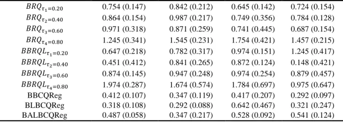
The (RMSE) and (MAE) are listed in Table 1. We can readily saw across all the quantile levels, our proposed methods (BBCQReg, BLBCQReg and BALBCQReg) have high performance compared to the BRQ and BBRQL. In general, Table (1) show that the (RMSE) and (MAE) for the proposed methods BBCQReg, BLBCQReg and BALBCQReg are smaller than that for existing methods.
Table 1. RMSE and MAE for the first simulation scenario Error distributions
𝐵𝑅𝑄𝜏1=0.20 0.754 (0.147) 0.842 (0.212) 0.645 (0.142) 0.724 (0.154) 𝐵𝑅𝑄𝜏2=0.40 0.864 (0.154) 0.987 (0.217) 0.749 (0.356) 0.784 (0.128) 𝐵𝑅𝑄𝜏3=0.60 0.971 (0.318) 0.871 (0.259) 0.741 (0.445) 0.687 (0.154) 𝐵𝑅𝑄𝜏4=0.80 1.245 (0.341) 1.545 (0.231) 1.754 (0.421) 1.457 (0.215) 𝐵𝐵𝑅𝑄𝐿𝜏1=0.20 0.647 (0.218) 0.782 (0.317) 0.974 (0.151) 1.245 (0.417) 𝐵𝐵𝑅𝑄𝐿𝜏2=0.40 0.451 (0.412) 0.841 (0.265) 0.872 (0.124) 0.148 (0.421) 𝐵𝐵𝑅𝑄𝐿𝜏3=0.60 0.874 (0.145) 0.947 (0.248) 0.974 (0.254) 0.879 (0.457) 𝐵𝐵𝑅𝑄𝐿𝜏4=0.80 1.974 (0.287) 1.674 (0.574) 1.784 (0.697) 0.975 (0.647) BBCQReg 0.412 (0.107) 0.347 (0.119) 0.417 (0.207) 0.292 (0.097) BLBCQReg 0.318 (0.108) 0.292 (0.088) 0.642 (0.467) 0.321 (0.247) BALBCQReg 0.487 (0.058) 0.347 (0.217) 0.528 (0.092) 0.541 (0.124) In the parentheses are belong to MAE.
3.2. Second simulation
In the second simulation scenario, we will used dense case within the true our model:
𝑦 𝑖 = 0.85𝑥𝑖1+ 0.85𝑥𝑖2+ 0.85𝑥𝑖3+ 0.85𝑥𝑖4+ 0.85𝑥𝑖5+ 0.85𝑥𝑖6+ 0.85𝑥𝑖7+ 0.85𝑥𝑖8
+ 𝜀𝑖 𝑤ℎ𝑒𝑟𝑒 𝑖 = 1. . .100
The independent variables also are generated from the standard Uniform (0,1). where the true parameters of independent variables, including the intercept, are 𝛽 = 0,0.85,0.85,0.85,0.85,0.85,0.85,0.85,0.85.
In Table 2, we show the summary of the RMSE and MAE for the five methods under study. From this table we can see that clearly our three proposed methods BBCQReg, BLBCQReg and BALBCQReg are get the smallest values of RMSE and MAE during all error distribution.
Table 2. RMSE and MAE for the second simulation scenario. Error distributions
Methods under study 𝜀𝑖~𝑁(0,1) 𝜀𝑖~Normal mix 𝜀𝑖~𝑡(3) 𝜀𝑖~𝐿𝑎𝑝(0,1) 𝐵𝑅𝑄𝜏1=0.20 0.865 (0.215) 0.926 (0.219) 0.743 (0.211) 0.682 (0.197) 𝐵𝑅𝑄𝜏2=0.40 0.925 (0.129) 0.869 (0.186) 0.795 (0.254) 0.659 (0.156) 𝐵𝑅𝑄𝜏3=0.60 0.828 (0. 398) 0.936 (0.359) 0.854 (0.523) 1.225 (0.524) 𝐵𝑅𝑄𝜏4=0.80 1.678 (0.354) 1.892 (0.245) 1.828(0.502) 1.871 (0.547) 𝐵𝐵𝑅𝑄𝐿𝜏1=0.20 0.781 (0.326) 0.745 (0.492) 0.624 (0.125) 0.598 (0.438) 𝐵𝐵𝑅𝑄𝐿𝜏2=0.40 0.645 (0.641) 0.648 (0.128) 0.846 (0.065) 0.648 (0.154) 𝐵𝐵𝑅𝑄𝐿𝜏3=0.60 0.924 (0.105) 0.862 (0.135) 0.792 (0.121) 0.754 (0.214) 𝐵𝐵𝑅𝑄𝐿𝜏4=0.80 2.542 (0.412) 1.524 (0.321) 1.421 (0.654) 1.135 (0.266) BBCQReg 0.354 (0.057) 0.451 (0.110) 0.531 (0.198) 0.311 (0.158) BLBCQReg 0.298 (0.175) 0.304 (0.091) 0.521 (0.350) 0.214 (0.114) BALBCQReg 0.385 (0.124) 0.218 (0.017) 0.124 (0.063) 0.411 (0.151) In the parentheses are belong to MAE
3.3. Third simulation
In the third simulation scenario, we will used sparse case with in the true our model: 𝑦 𝑖= 3𝑥𝑖1+ 𝑥𝑖2+ 𝑥𝑖5+ 𝜀𝑖 𝑤ℎ𝑒𝑟𝑒 𝑖 = 1. . .100
Similar to second Simulation the independent variables also are generated from the standard Uniform (0,1). Where the true parameters of independent variables, including the intercept, are 𝛽 = 0,3,1,0,0,1,0,0,0.
Table 3. RMSE and MAE for the third simulation scenario. Error distributions
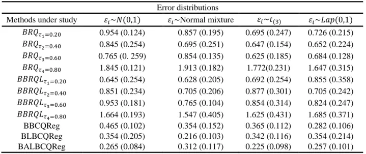
Methods under study 𝜀𝑖~𝑁(0,1) 𝜀𝑖~Normal mixture 𝜀𝑖~𝑡(3) 𝜀𝑖~𝐿𝑎𝑝(0,1) 𝐵𝑅𝑄𝜏1=0.20 0.954 (0.124) 0.857 (0.195) 0.695 (0.247) 0.726 (0.215) 𝐵𝑅𝑄𝜏2=0.40 0.845 (0.254) 0.695 (0.251) 0.647 (0.154) 0.652 (0.224) 𝐵𝑅𝑄𝜏3=0.60 0.765 (0. 259) 0.854 (0.135) 0.625 (0.185) 0.684 (0.128) 𝐵𝑅𝑄𝜏4=0.80 1.845 (0.121) 1.913 (0.182) 1.772(0.231) 1.647 (0.315) 𝐵𝐵𝑅𝑄𝐿𝜏1=0.20 0.645 (0.254) 0.628 (0.205) 0.692 (0.254) 0.855 (0.358) 𝐵𝐵𝑅𝑄𝐿𝜏2=0.40 0.851 (0.234) 0.705 (0.206) 0.877 (0.301) 0.705 (0.242) 𝐵𝐵𝑅𝑄𝐿𝜏3=0.60 0.953 (0.181) 0.765 (0.104) 0.854 (0.314) 0.824 (0.247) 𝐵𝐵𝑅𝑄𝐿𝜏4=0.80 1.664 (0.193) 1.547 (0.405) 1.625 (0.431) 1.685 (0.371) BBCQReg 0.465 (0.102) 0.354 (0.152) 0.365 (0.112) 0.282 (0.106) BLBCQReg 0.354 (0.205) 0.216 (0.103) 0.342 (0.116) 0.354 (0.214) BALBCQReg 0.265 (0.084) 0.312 (0.117) 0.225 (0.098) 0.257 (0.101)
In the parentheses are belong to MAE.
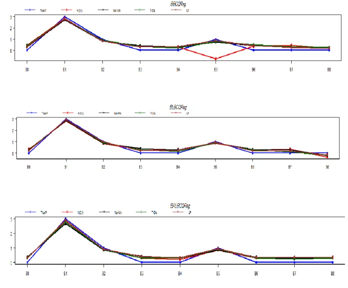
As same as Table 1 and Table 2, Table 3 show the values of RMSE and MAE of all methods proposed and existing. This table showing that proposed methods BBCQReg, BLBCQReg and BALBCQReg are better than the other existing methods BRQ and BBRQL. Whereas the results showing that the RMSE and MAE for the proposed methods BBCQReg, BLBCQReg and BALBCQReg are smaller than that for the other methods existing method (BRQ and BBRQL). In this paper, we will use another procedure for the evaluating the methods under study is parameters estimations in direct way. Figure 1 shows plot of parameter estimations in the second simulation. From the Figure 1, it can see that our proposed methods are estimated the parameters very close to the true parameters compared with other methods. As the result, our proposed methods have high efficiency compared with previous methods.
Figure 1. Plot of parameter estimations in in direct way for the second simulation to the methods under study.
4. Real data
To clarification our proposed methods for (BBCQReg, BLBCQReg and BALBCQReg) and compare with 𝐵𝑅𝑄 and 𝐵𝐵𝑅𝑄𝐿 approaches, the data of Pima Indians have been considered, these data set available in the caret package in R programs, from [23]. The Pima Indians Diabetes data consists of (532) observations of which 200 are test positive observations and 332 are test positive observations. The important part in the study of Pima Indians is in achieving the relationship between diabetic according to WHO criteria, (diabetes) and eight independent variables. The seven independent variables are 𝑋1: Number of pregnancies code by (npreg), 𝑋2: Plasma glucose concentration in an oral glucose tolerance test code by (glu), 𝑋3: diastolic blood pressure (mm Hg) code by (bp), 𝑋4: triceps skin fold thickness (mm) code by (skin), 𝑋5: body mass index (weight in kg/(height in m)\^2) code by (bmi), 𝑋6: diabetes pedigree function code by (ped) and 𝑋7: age in years code by (age).
As same as Section three, in this section we compare our proposed methods with the previous two existing methods are assessed based on the mean squared error (MSE).
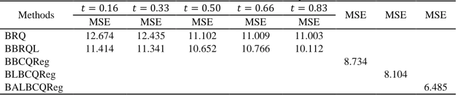
Table 4. MSE for the methods under comparison
Methods 𝑡 = 0.16 𝑡 = 0.33 𝑡 = 0.50 𝑡 = 0.66 𝑡 = 0.83 MSE MSE MSE
MSE MSE MSE MSE MSE
BRQ 12.674 12.435 11.102 11.009 11.003
BBRQL 11.414 11.341 10.652 10.766 10.112
BBCQReg 8.734
BLBCQReg 8.104
BALBCQReg 6.485
From the results are listed in Table 4, the MSE of our proposed methods Bayesian Binary composite quantile regression model, Bayesian lasso penalty for binary composite quantile regression and Bayesian adaptive lasso penalty for binary composite quantile regression are 8.734,8.104 and 6.485 respectively. Where, the MSE generated by our proposed methods are much smaller than MSE generated by BRQ and BBRQL methods via all quantile levels. So, our methods have performance better than previous methods (BRQ and BBRQL).
5. Conclusion
In this paper, Bayesian binary composite quantile regression approach is proposed for estimating the model. In binary composite quantile regression lasso and the adoptive lasso penalty are considered for selecting variables in a Bayesian framework. We developed a Bayesian hierarchical model for the lasso and adaptive lasso penalty methods, whereas Gibbs sampler algorithm was adopted for posterior inference.
Simulation examples and real data were considered to compare our proposed methods BBCQReg, BLBCQReg and BALBCQReg with other methods, BRQ and BBRQL with different quantiles. Based on the simulation scenarios the RMSE and MAE of our proposed methods BBCQReg, BLBCQReg and BALBCQReg are smaller than the RMSE and MAE of the other existing methods BRQ and BBRQL.
The numerical study signify that the proposed methods offers substantial improvement over the other two methods. So that, we concluded that our proposed methods perform better than the other two existing methods.
References
[1] J. Abrevaya, “The effects of demographics and maternal behavior on the distribution of birth outcomes,”
Economic applications of quantile regression (pp. 247-257). Physica, Heidelberg, 2002.
[2] R. Alhamzawi, and K. Yu, “Bayesian Lasso-mixed quantile regression.” Journal of Statistical
Computation and Simulation, vol. 84, no. 4, p. 868-880. 2014.
[3] R. Alhamzawi, K. Yu, and D. F. Benoit, “Bayesian adaptive Lasso quantile regression.” Statistical
Modelling, vol. 12, no. 3, p. 279-297, 2012.
[4] D. F. Andrews, and C. L. Mallows, “Scale mixtures of normal distributions.” Journal of the Royal
Statistical Society: Series B (Methodological), vol. 36, no.1, p. 99-102, 1974.
[5] D. F. Benoit, and D. Van den Poel,” Binary quantile regression: A Bayesian approach based on the asymmetric Laplace distribution.” Journal of Applied Econometrics, vol. 27, no.7, p. 1174-1188, 2012. [6] D. F. Benoit, R. Alhamzawi and K. Yu, “Bayesian lasso binary quantile regression.” Computational
Statistics, vol. 28, no. 6, p. 2861-2873, 2013.
[7] S. A. Campbell, and Y. Yuan,” Zero singularities of codimension two and three in delay differential equations.” Nonlinearity, vol. 21, no. 11, p. 2671-2691, 2008.
[8] J. Fan, and R. Li, “Variable selection via nonconcave penalized likelihood and its oracle properties.” Journal of the American statistical Association, vol. 96, no.456, p. 1348-1360, 2001.
[9] J. L. Horowitz, “A smoothed maximum score estimator for the binary response model.” Econometrica:
Journal of the Econometric Society, vol. 60, no. 3, p. 505-531, 1992.
[10] H. Huang, and Z. Chen, “Bayesian composite quantile regression.” Journal of Statistical Computation
and Simulation, vol. 85, no. 18, p. 3744-3754, 2015.
[11] K. Khare, and J. P. Hobert, “Geometric ergodicity of the Gibbs sampler for Bayesian quantile regression.” Journal of Multivariate Analysis, vol. 112, p. 108-116, 2012.
[12] R. Koenker, “Quantile regression for longitudinal data.” Journal of Multivariate Analysis, vol. 91, no. 1, p. 74-89, 2004.
[13] R. Koenker, and V. D'Orey, “Algorithm AS 229: Computing regression quantiles.” Journal of the
Royal Statistical Society. Series C (Applied Statistics), vol. 36, no. 3, p. 383-393, 1987.
[14] R. Koenker, and JR. Bassett,” Regression quantiles.” Econometrica: journal of the Econometric Society, vol. 46, no. 1, p. 33-50, 1978.
[15] R. Koenker, and J. A. Machado, “Goodness of fit and related inference processes for quantile regression.” Journal of the american statistical association, vol. 94, no. 448, p. 1296-1310, 1999. [16] G. Kordas, “Smoothed binary regression quantiles.” Journal of Applied Econometrics, vol. 21, no. 3, p.
387-407, 2006.
[17] H. Kozumi, & G. Kobayashi, “Gibbs sampling methods for Bayesian quantile regression.” Journal of
statistical computation and simulation, vol. 81, no. 11, p. 1565-1578, 2011.
[18] Q. Li, R. Xi, and N. Lin, “Bayesian regularized quantile regression.” Bayesian Analysis, vol. 5, no. 3, p. 533-556, 2010.
[19] Y. Li, and J. Zhu, “L1-norm quantile regression.” Journal of Computational and Graphical
Statistics, vol. 17, no.1, p.163-185, 2008.
[20] C. F. Manski, “Maximum score estimation of the stochastic utility model of choice.” Journal of
econometrics, vol. 3, no. 3, 205-228, 1975.
[21] C. F. Manski, “Semiparametric analysis of discrete response: Asymptotic properties of the maximum score estimator.” Journal of econometrics, vol. 27, no. 3, p. 313-333, 1985.
[22] V. L. Miguéis, D. F. Benoit, and D. Van den Poel, “Enhanced decision support in credit scoring using Bayesian binary quantile regression.” Journal of the Operational Research Society, vol. 64, no. 9, p. 1374-1383, 2013.
[23] J. W. Smith, J. E. Everhart, W. C. Dickson, W. C. Knowler, and R. S. Johannes, “Using the ADAP learning algorithm to forecast the onset of diabetes mellitus.” Proceedings of the Annual Symposium on
Computer Application in Medical Care, p. 261-265, Nov. 1988.
[24] R. Tibshirani, “Regression shrinkage and selection via the lasso.” Journal of the Royal Statistical
Society: Series B (Methodological), vol. 58, no. 1, p. 267-288., 1996.
[25] K. Yu, and R. A. Moyeed, “Bayesian quantile regression.” Statistics & Probability Letters, vol. 54, no. 4, p. 437-447, 2001.
[26] K. Yu, Z. Lu, & J. Stander, “Quantile regression: applications and current research areas.” Journal of
the Royal Statistical Society: Series D (The Statistician), vol. 52, no. 3, p. 331-350, 2003.
[27] Z. Zhao, and Z. Xiao, “Efficient regressions via optimally combining quantile information.” Econometric theory, vol. 30, no. 6, p. 1272-1314, 2014.
[28] H. Zou, “The adaptive lasso and its oracle properties.” Journal of the American statistical
association, vol. 101, no. 476, p. 1418-1429, 2006.
[29] H. Zou, and T. Hastie, “Regularization and variable selection via the elastic net.” Journal of the royal
[30] H. Zou, and M. Yuan, “Composite quantile regression and the oracle model selection theory.” The
Annals of Statistics, vol. 36, no. 3, 1108-1126, 2008.
Appendix
I. Gibbs sampler Bayesian binary composite quantile regression
The conditional distribution 𝑓(𝛽𝑘|𝑦 𝑖, 𝑋, 𝛽−𝑘, 𝑏𝜏, 𝑢𝑖, 𝑤, 𝑘), where 𝛽−𝑘 is the parameters vector excepting 𝛽𝑘 , is normal 𝑓(𝛽𝑘|𝑦 𝑖, 𝑋, 𝛽−𝑘, 𝑏, 𝑢, 𝑤, 𝐾) ∝ 𝑓(𝑦 𝑖|𝑋, 𝛽, 𝑏, 𝑢, 𝑤, 𝐾) × 𝜋(𝛽) ∝ 𝑒𝑥𝑝 {−1 2[∑ 𝑛 𝑖=1 (50𝑥𝑖𝑘′2+ 𝑢𝑖) 100𝑢𝑖 𝛽𝑘2− 2 ∑ 𝑛 𝑖=1 50𝑦 𝑖∗𝑥𝑖𝑘′ 100𝑢𝑖 𝛽𝑘]} ∝ 𝑁 [ ∑𝑛𝑖=1 (50𝑘𝑖𝑗𝑦 𝑖 ∗𝑥 𝑖𝑘 100𝑢𝑖) ∑𝑛 𝑖=1 ( (50𝑘𝑖𝑗𝑥𝑖𝑘2 + 𝑢𝑖) 100𝑢𝑖) , 1 ∑𝑛 𝑖=1 ( (50𝑘𝑖𝑗𝑥𝑖𝑘2 + 𝑢𝑖) 100𝑢𝑖) ] 𝑦 𝑖∗= 𝑦 𝑖− 𝑏𝜏𝑗− 𝑥𝑖,−𝑘′ 𝛽−𝑘− 𝜃𝑢𝑖
The conditional distribution 𝑓( 𝑢𝑖|𝑦 𝑖, 𝑋, 𝛽, 𝑏 , 𝑢−𝑖, 𝑤, 𝐾) , where 𝑢−𝑖 is the variable 𝑢 excepting the component 𝑢𝑖 is given by 𝑓(𝑢𝑖|𝑦 𝑖, 𝑋, 𝛽, 𝑏 , 𝑢−𝑖, 𝑤, 𝐾) ∝ 𝑓(𝑦 𝑖|𝑋, 𝛽, 𝑏, 𝑢, 𝑤, 𝐾) × 𝜋(𝑢𝑖|𝜏) ∝ (𝑢𝑖) −1 2 𝑒𝑥𝑝 {−1 2∑ 𝑞 𝑗=1 𝑘𝑖𝑗[( (𝑦 𝑖−𝑏𝜏−𝑥𝑖′𝛽 ) 2 2 ) 𝑢𝑖 −1+ (𝜃2 2 + 2𝜏(1 − 𝜏))𝑢𝑖]}
So the conditional distribution of 𝑢𝑖 is generalized inverse Gaussian 𝐺𝐼𝐺(𝑢𝑖, 𝐴, 𝐵) where 𝐴 =
(𝑦 𝑖−𝑏𝜏−𝑥𝑖′𝛽 ) 2
2 and
𝐵 =𝜃2
2 + 2𝜏(1 − 𝜏).
The conditional distribution 𝑓(𝑏𝜏𝑘|𝑦 𝑖, 𝑋, 𝛽, 𝑏−𝜏𝑘, 𝑢, 𝑤, 𝐾) is a normal distribution 𝑓( 𝑏𝜏𝑘|𝑦 𝑖, 𝑋, 𝛽, 𝑏−𝜏𝑘, 𝑢, 𝑤, 𝐾) ∝ 𝑓(𝑦 𝑖|𝑋, 𝛽, 𝑏, 𝑢, 𝑤, 𝐾) ∝ 𝑒𝑥𝑝 {−1 2[∑ 𝑛 𝑖=1 𝑘𝑖𝑗 2𝑢𝑖 𝑏𝜏𝑘 2 − 2 ∑ 𝑛 𝑖=1 𝑘𝑖𝑗𝑦 𝑖∗∗ 2𝑢𝑖 𝑏𝜏𝑘]} ∝ 𝑁 ( ∑𝑛𝑖=1 ( 𝑘𝑖𝑗𝑦 𝑖∗∗ 2𝑢𝑖) ∑𝑛 𝑖=1 ( 𝑘𝑖𝑗 2𝑢𝑖) , 1 ∑𝑛 𝑖=1 ( 𝑘𝑖𝑗 2𝑢𝑖)) 𝑦 𝑖∗∗= 𝑦 𝑖− 𝑥𝑖′𝛽 − 𝜃𝑢𝑖
Follow [10] the conditional distribution 𝑓(𝑤|𝑦̌𝑖, 𝑋, 𝛽, 𝑏, 𝑢, 𝐾) is given as follow 𝑓(𝑤|𝑋, 𝑦 𝑖, 𝛽, 𝑏𝜏𝑘, 𝑢𝑖, 𝑘) 𝛼 ∏ 𝑞 𝑗=1 𝑤𝑗𝑛𝑗+𝛿𝑗 ∝ 𝐷𝑖𝑟𝑖𝑐ℎ𝑙𝑒𝑡(𝑛1+ 𝛿1, … … … … . . , 𝑛𝑞+ 𝛿𝑞) Where 𝑛𝑗 is the summation of the objects 𝑘𝑖𝑗 in the 𝑗𝑡ℎ cluster, i.e. ∑𝑛𝑖=1 𝑘𝑖𝑗. The conditional distribution 𝑓(𝑘𝑖| 𝑋, 𝑦 𝑖, 𝛽, 𝑏, 𝑢, 𝑤, 𝑘−𝑖) can be shown as ([10])
𝑓(𝑘𝑖| 𝑋, 𝑦 𝑖, 𝛽, 𝑏, 𝑢, 𝑤, 𝑘−𝑖) ∝ ∏ 𝑞 𝑗=1 {𝑤𝑗𝑒𝑥𝑝 [− 1 4𝑢𝑖 (𝑦 𝑖− 𝑏𝜏𝑗− 𝑥𝑖 ′𝛽 − 𝜃𝑢 𝑖) 2 ]} 𝑘𝑖𝑗 ∝ 𝑀𝑖𝑙𝑡𝑖𝑛𝑜𝑚𝑖𝑎𝑙 (1, 𝑝̂1, … … … . . , 𝑝̂𝑞) Where 𝑝̂𝑗 = 𝑤𝑗𝑒𝑥𝑝 [−4𝑢1 𝑖(𝑦 𝑖− 𝑏𝜏𝑗− 𝑥𝑖 ′𝛽 − 𝜃𝑢 𝑖) 2 ] ∑𝑞𝑗=1 𝑤𝑗𝑒𝑥𝑝 [−4𝑢1 𝑖(𝑦 𝑖− 𝑏𝜏𝑗− 𝑥𝑖 ′𝛽 − 𝜃𝑢 𝑖) 2 ] II. Gibbs sampler Bayesian lasso binary composite quantile regression:
The conditional distribution of 𝑢, 𝑏, 𝑤 and 𝐾 will be as same as that in Appendix I. The conditional distribution of 𝛾2 is a Gamma distribution
𝑓(𝛾2| 𝑋, 𝑦 𝑖, 𝛽, 𝑏, 𝑢, 𝑠, 𝑤, 𝐾) 𝛼 𝑓(𝑠|𝛾2) × 𝜋(𝛾2) ∝ (𝛾2)𝑝+𝑎−1𝑒𝑥𝑝 {−(1 2∑ 𝑝 𝑘=1 𝑠𝑘+ 𝑏)𝛾2} ∝ 𝐺𝑎𝑚𝑚𝑎(𝑝 + 𝑎,1 2∑ 𝑝 𝑘=1 𝑠𝑘+ 𝑏)
The conditional distribution 𝑓(𝛽𝑘|𝑋, 𝑦 𝑖, 𝛽−𝑘, 𝑏, 𝑢, 𝑠, , 𝛾2, 𝑤, 𝐾), where 𝛽−𝑘 is a parameters vector excepting 𝛽𝑘 is a normal distribution 𝑓(𝛽𝑘|𝑋, 𝑦 𝑖, 𝛽−𝑘, 𝑏, 𝑢, 𝑠, , 𝛾2, 𝑤, 𝐾)𝛼 𝑓(𝑦 𝑖|𝑋, 𝛽, 𝑏, 𝑢, 𝑠, , 𝛾2, 𝑤, 𝐾) × 𝜋(𝛽𝑘|𝑠𝑘) ∝ 𝑒𝑥𝑝 {−1 2[(∑ 𝑞 𝑗=1 ∑ 𝑛 𝑖=1 𝑘𝑖𝑗𝑥𝑖𝑘2 2𝑢𝑖 + 1 𝑠𝑘 )𝛽𝑘2− 2 ∑ 𝑞 𝑗=1 ∑ 𝑛 𝑖=1 𝑘𝑖𝑗𝑥𝑖𝑘𝑦 𝑖∗ 2𝑢𝑖 𝛽𝑘 ]}
∝ 𝑁 [ ∑𝑞𝑗=1 ∑𝑛𝑖=1 (𝑘𝑖𝑗𝑥𝑖𝑘𝑦 𝑖 ∗ 2𝑢𝑖 ) ∑𝑞𝑗=1 ∑𝑛 𝑖=1 ( 𝑘𝑖𝑗𝑥𝑖𝑘2 2𝑢𝑖 ) + ( 1 𝑠𝑘) , 1 ∑𝑞𝑗=1 ∑𝑛 𝑖=1 ( 𝑘𝑖𝑗𝑥𝑖𝑘2 2𝑢𝑖 ) + ( 1 𝑠𝑘)] 𝑦 𝑖 = 𝑦 𝑖− 𝑏𝜏𝑗− 𝑥𝑖,−𝑘 ′ 𝛽 −𝑘− 𝜃𝑢𝑖
The conditional distribution 𝑓(𝑠𝑘|𝑋, 𝑦 𝑖, 𝛽, 𝑏, 𝑢, 𝑠−𝑘, 𝛾2, 𝑤, 𝐾), where 𝑠−𝑘 is the variable 𝑠 excepting the component 𝑠𝑘 is generalized inverse Gaussian
𝑓(𝑠𝑘|𝑋, 𝑦 𝑖, 𝛽, 𝑏, 𝑢, 𝑠−𝑘, 𝛾2, 𝑤, 𝐾)𝛼 𝜋(𝑠𝑘|𝛾2) × 𝜋(𝛽𝑘|𝛾2) ∝ 𝑠𝑘− 1 2𝑒𝑥𝑝 𝑒𝑥𝑝 {−1 2(𝛽𝑘 2𝑠 𝑘−1+ 𝛾2𝑠𝑘)} 𝛼 𝐺𝐼𝐺(𝑠𝑘, 𝛽𝑘 2, 𝛾2)
III. Gibbs sampler Bayesian adaptive lasso binary composite quantile regression
As same as we mentioned in Appendix II the conditional distribution for 𝑢, 𝑏, 𝑤 and 𝐾 will not be change. The conditional distribution of 𝜂𝑘2 is a Gamma distribution and derivative as follows
𝑓(𝜂𝑘2/ 𝑋, 𝑦 𝑖, 𝛽, 𝑏, 𝑢𝑖, 𝑟, 𝜂−𝑘2 , 𝑤, 𝑘) ∝ 𝑓(𝑟|𝜂𝑘2) × 𝜋(𝜂𝑘2|𝑐, 𝑑) ∝ (𝜂𝑘2) 𝑐 𝑒𝑥𝑝 𝑒𝑥𝑝 (− (𝑟𝑘 2 + 𝑑) 𝜂𝑘 2) ∝ 𝐺𝑎𝑚𝑚𝑎 (𝑐 + 1, (𝑟𝑘 2 + 𝑑))
The conditional distribution 𝑓( 𝑟𝑘/ 𝑋, 𝑦 𝑖, 𝛽, 𝑏, 𝑢, 𝑟−𝑘, 𝜂𝑘2, 𝑤, 𝑘), where 𝑟−𝑘 is the variable 𝑟 excepting the component 𝑟𝑘 is a generalized inverse Gamma distribution and given by
𝑓( 𝑟𝑘/ 𝑋, 𝑦 𝑖, 𝛽, 𝑏, 𝑢𝑖, 𝑟−𝑘, 𝜂2𝑘, 𝑤, 𝑘) 𝛼 𝑓(𝑟𝑘|𝜂𝑘2) × 𝜋(𝛽𝑘|𝜂𝑘2) ∝ (𝑟𝑘)− 1 2𝑒𝑥𝑝 {−1 2( 𝛽𝑘 2𝑟 𝑘−1+ 𝜂𝑘2𝑟𝑘) 𝛼 𝐺𝐼𝐺(𝑟𝑘, 𝛽𝑘 2, 𝜂𝑘2)
The conditional distribution of 𝛽𝑘 is a normal distribution and shown as follow:
∝ 𝑒𝑥𝑝 {−1 2[(∑ 𝑞 𝑗=1 ∑ 𝑛 𝑖=1 𝑘𝑖𝑗𝑥𝑖𝑘2 2𝑢𝑖 + 1 𝑟𝑘 )𝛽𝑘2− 2 ∑ 𝑞 𝑗=1 ∑ 𝑛 𝑖=1 𝑘𝑖𝑗𝑥𝑖𝑘𝑦 𝑖∗ 2𝑢𝑖 𝛽𝑘 ]} ∝ 𝑁 [ ∑𝑞𝑗=1 ∑𝑛 𝑖=1 ( 𝑘𝑖𝑗𝑥𝑖𝑘𝑦 𝑖 ∗ 2𝑢𝑖 ) ∑𝑞𝑗=1 ∑𝑛 𝑖=1 ( 𝑘𝑖𝑗𝑥𝑖𝑘2 2𝑢𝑖 ) + ( 1 𝑟𝑘) , 1 ∑𝑞𝑗=1 ∑𝑛 𝑖=1 ( 𝑘𝑖𝑗𝑥𝑖𝑘2 2𝑢𝑖 ) + ( 1 𝑟𝑘)] 𝑦 𝑖∗= 𝑦 𝑖− 𝑏𝜏𝑗− 𝑥𝑖,−𝑘 ′ 𝛽 −𝑘− 𝜃𝑢𝑖