Shift-based density estimation for pareto-based algorithms in many-objective optimization

(1)

Shift-Based Density Estimation for Pareto-Based

Algorithms in Many-Objective Optimization

Miqing Li, Shengxiang Yang

Member, IEEE,

and Xiaohui Liu

Abstract—It is commonly accepted that Pareto-based evolu-tionary multiobjective optimization (EMO) algorithms encounter difficulties in dealing with many-objective problems. In these algorithms, the ineffectiveness of the Pareto dominance relation for a high-dimensional space leads diversity maintenance mech-anisms to play the leading role during the evolutionary process, while the preference of diversity maintenance mechanisms for individuals in sparse regions results in the final solutions dis-tributed widely over the objective space but distant from the desired Pareto front. Intuitively, there are two ways to address this problem: 1) modifying the Pareto dominance relation and 2) modifying the diversity maintenance mechanism in the algorithm. In this paper, we focus on the latter and propose a shift-based density estimation (SDE) strategy. The aim of our study is to develop a general modification of density estimation in order to make Pareto-based algorithms suitable for many-objective optimization. In contrast to traditional density estimation which only involves the distribution of individuals in the population, SDE covers both the distribution and convergence information of individuals. The application of SDE in three popular Pareto-based algorithms demonstrates its usefulness in handling many-objective problems. Moreover, an extensive comparison with five state-of-the-art EMO algorithms reveals its competitiveness in balancing convergence and diversity of solutions. These findings not only show that SDE is a good alternative to tackle many-objective problems, but also present a general extension of Pareto-based algorithms in many-objective optimization.

Index Terms—Evolutionary multiobjective optimization, many-objective optimization, shift-based density estimation, conver-gence, diversity.

I. INTRODUCTION

O

VER the past few decades, evolutionary algorithms (EAs) have attracted great attention in solving a class of real-world problems that have several competing crite-ria or objectives. The involved EAs are called evolutionary multiobjective optimization (EMO) algorithms. One of the important reasons for the success of EMO algorithms is due to their ability of achieving a Pareto approximation set of multiobjective optimization problems (MOPs) in a single run. In general, an EMO algorithm, in the absence of any further information provided by the decision maker, pursues two ultimate goals with respect to its solution set—minimizing the distance to the Pareto front (i.e., convergence) and maximizing the distribution over the Pareto front (i.e., diversity) [15].

Most EMO algorithms are designed with regard to the above two common goals, but different algorithms are implemented

M. Li and X. Liu are with the Department of Information Systems and Computing, Brunel University, Uxbridge, Middlesex UB8 3PH, U. K. (email:

{miqing.li, xiaohui.liu}@brunel.ac.uk).

S. Yang is with the Centre for Computational Intelligence (CCI), School of Computer Science and Informatics, De Montfort University, Leicester LE1 9BH, U. K. (e-mail: [email protected]).

to achieve them in distinct ways. So far, EMO algorithms, based on their selection mechanisms, can be generally classi-fied into three groups—Pareto-based algorithms, aggregation-based algorithms, and indicator-aggregation-based algorithms [10], [71].

Since the optimal outcome of an MOP is a set of Pareto optimal solutions, the Pareto dominance relation naturally becomes a criterion to distinguish solutions during the evo-lutionary process of an algorithm. Behind such Pareto-based algorithms, the basic idea is to compare solutions according to their dominance relation and density. The former is considered as the primary selection and favors nondominated solutions over dominated ones, and the latter is used to maintain diver-sity and is activated when solutions are incomparable using the primary selection. Most of the existing EMO algorithms belong to this group, and among them, several representative algorithms, such as the nondominated sorting genetic algo-rithm II (NSGA-II) [13], strength Pareto EA 2 (SPEA2) [81], and Pareto envelope-based selection algorithm II (PESA-II) [11], are being widely applied to various problem domains [69], [73], [80].

In aggregation-based algorithms, the objectives of an MOP are aggregated by a scalarizing function such that a single scalar value is generated. The diversity of a population is main-tained by specifying a set of well-distributed reference points (or directions) to guide its individuals to search simultaneously towards different directions [64]. As the earliest multiobjective optimization approach that can be traced back to the middle of the last century [51], this group has become popular again in recent years. One of the important reasons is due to the appearance of an efficient algorithm, the decomposition-based multiobjective EA (MOEA/D) [79].

The idea of indicator-based EMO algorithms, which was first introduced by Zitzler and K¨unzli [84], is to utilize a performance indicator to guide the search during the evolu-tionary process. An interesting characteristic is that, in contrast to Pareto-based algorithms that compare individuals using two criteria (i.e., dominance relation and density), indicator-based algorithms adopt a single indicator to optimize a desired property of the evolutionary population. The indicator-based EA (IBEA) [84] is a pioneer in this group. Recently, the indicator hypervolume [82] has been found to be promising in balancing convergence and diversity, leading to the popu-larity of several hypervolume-based algorithms, such as the

S metric selection EMO algorithm (SMS-EMOA) [5] and multiobjective covariance matrix adaptation evolution strategy (MO-CMA-ES) [34]. Whereas a large computation cost is required in the calculation of the hypervolume indicator, some efforts to address this issue are being made [7], [74].

(2)

Many-objective optimization refers to the simultaneous op-timization of more than three objectives. In the last decade, many-objective optimization has gained growing attention in the EMO community [12], [24], [39], [57]. One of the impor-tant reasons is due to the rapid increase of difficulties with the number of objectives in multiobjective optimization [8], [68], [70]. Most current EMO algorithms, which work well on problems with two or three objectives, noticeably deteriorate their search ability when more objectives are involved [46], [48], [65]. This greatly motivates researchers to design new algorithms specially for many-objective problems. Recently, some reports have shown that algorithms based on the design idea of group 2 or group 3 (i.e., aggregation-based or indicator-based algorithms) are very competitive in many-objective optimization [33], [38], [71]. In this regard, Hughes’s multiple single objective Pareto sampling (MSOPS) [32] and Bader and Zitzler’s hypervolume estimation algorithm (HypE) [4] are two representatives.

Despite being the most popular approaches in the EMO community, Pareto-based algorithms encounter difficulties in their scalability to many-objective optimization. Most classical Pareto-based algorithms, such as NSGA-II and SPEA2, cannot provide sufficient selection pressure towards the Pareto front for most many-objective optimization problems1_{. A major}

reason is that the proportion of nondominated solutions in a population tends to become large as the number of objectives increases. This makes the Pareto dominance relation-based primary selection criterion fail to distinguish solutions and the density-based second selection criterion play a leading role in both the mating and environmental selection of an algorithm. This phenomenon is termedactive diversity promotionin Pur-shouse and Fleming’s study [65]. Some empirical observations [39], [71] indicate that the active diversity promotion has a detrimental impact on the algorithm’s convergence due to its preference for dominance resistant solutions [35] (i.e., the solutions with an extremely poor value in at least one of the objectives, but with near optimal values in some others). Consequently, the solutions, at the end of the optimization process, may have “good” diversity over the objective space, but can be far away from the desired Pareto front.

Intuitively, there are two ways to deal with the issue that Pareto-based algorithms face in many-objective optimization. One is related to the primary selection criterion (i.e., modi-fying the Pareto dominance relation to make more solutions comparable), and the other is concerned with the second selection criterion (i.e., modifying the diversity maintenance mechanism to weaken or avoid the active diversity promotion phenomenon).

Much of the current work is on the primary selection crite-rion, introducing a variety of new dominance concepts to solve many-objective problems, e.g., dominance area control [67],

k-optimality [23], preference order ranking [21], subspace dominance comparison [2], [44], and grid dominance [77]. These enhanced dominance relations can significantly increase 1_{Pareto-based EMO algorithms can work well on some many-objective}

problems where the Pareto front is on a low-dimensional subspace of the high-dimensional objective space [68], or the objectives are highly correlated and/or dependent [36], [41].

the selection pressure among solutions, thereby guiding the search towards the desired direction [12], [43]. In addition, several classical concepts which are not particularly designed for many-objective problems, such as ϵ-dominance [54] and fuzzy Pareto dominance [49], have also been shown to provide competitive results [19], [28], [50].

In sharp contrast to the above, the work on the second selection criterion has received little attention so far. To the best of the authors’ knowledge, there are only two approaches that concern improving the diversity maintenance mechanism. Adra and Fleming [1] employed a diversity management operator (DMO) to adjust the diversity requirement in the mat-ing and environmental selection. By comparmat-ing the boundary values between the current population and the Pareto front, the diversity maintenance mechanism is controlled (i.e., activated or inactivated) during the evolutionary process. Wagner et al. [71] demonstrated that assigning the crowding distance

of boundary solutions a zero value in NSGA-II can clearly improve the performance in terms of convergence, despite the risk of losing diversity among solutions [38].

This paper focuses on the second selection criterion for Pareto-based algorithms. The aim of our study is to develop a general modification of the second selection criterion in order to make Pareto-based algorithms suitable for many-objective optimization. To this end, a shift-based density estimation (SDE) strategy is proposed. In contrast to traditional density estimation which only involves the distribution of individuals in the population, SDE covers both the distribution and conver-gence information of individuals. When estimating the density of the surrounding area of an individual in the population, SDE shifts the position of other individuals according to their convergence comparison in order to reflect the relative proximity of the individual to the Pareto front.

The basic idea of SDE is simple—given the preference of density estimators for individuals in sparse regions, SDE tries to “put” individuals with poor convergence into crowded regions. This way, these poorly-converged individuals will be assigned a high density value, thus being eliminated easily during the evolutionary process. In addition, the implementa-tion of SDE is also simple, with negligible computaimplementa-tional cost, and it can be applied to any specific density estimator without the need of additional parameters.

The rest of this paper is organized as follows. Sect. II is devoted to the analysis of traditional density estimation in many-objective optimization, the description of the pro-posed method, and the application of SDE to three popular Pareto-based algorithms, i.e., NSGA-II, SPEA2, and PESA-II. Sect. III experimentally validates the proposed SDE based on its implementation into the three aforementioned Pareto-based algorithms, resulting in three new EMO algorithms, denoted NSGA-II+SDE, SPEA2+SDE, and PESA-II+SDE, respectively. In Sect. IV, a further test is carried out to compare one of the three obtained EMO algorithms with five state-of-the-art algorithms in many-objective optimization. Some discussions regarding the proposed method are given in Sect. V. Finally, Sect. VI draws the conclusions of this paper.

(3)

II. THEPROPOSEDMETHOD

A. Density Estimation in EMO Algorithms

In a population, the density of an individual represents the degree of crowding of the area where the individual is located. Due to the close relation with diversity maintenance, density estimation is very important in EAs and is widely applied in various optimization scenarios, such as multimodal optimization [62], dynamic optimization [76], and robustness optimization [45].

In multiobjective optimization, usually there is no single optimal solution but rather a set of Pareto optimal solutions. Naturally, density estimation plays a fundamental role in the evolutionary process of multiobjective optimization for an algorithm to obtain a representative and diverse subset of the Pareto front [6], [53].

There are a wide range of density estimation techniques that have been developed in the EMO community. They act on different neighbors of an individual, involve different neigh-borhoods, and consider different measures [47]. For example, the niched Pareto genetic algorithm (NPGA) considers the niche of an individual and measures the degree of crowding in the niche [30]. The strength Pareto EA (SPEA) uses a clustering technique to estimate the crowding degree of an individual [82]. NSGA-II defines a new measure, “crowding distance”, to reflect the density of an individual, only acting on the two closest neighbors located in either side for each objective. Most grid-based EMO approaches, such as PESA-II and the dynamic multiobjective EA (DMOEA) [78], estimate the density of an individual by counting the individuals in the hyperbox where it is located [56]; yet some recent grid-based approaches consider the crowding degree of a region constructed by a set of hyperboxes whose range varies with the number of objectives [59], [60]. SPEA2 considers the k -th nearest neighbor of an individual in -the population [81]. Instead of using the Euclidean distance in SPEA2, Horoba and Neumann used the Tchebycheff distance to determine thek-th nearest neighbor [31]. In [58], a Euclidean minimum spanning tree (EMST) of individuals in a population is generated, and the density of an individual is estimated by its edges in the EMST. Farhang-Mehr and Azarm calculated the entropy in the population, estimating the density of an individual by considering the influences coming from all other individuals in the population [22].

Despite the variety of density estimation techniques, they all measure the similarity degree among individuals in the population, i.e., they estimate the density of an individual by considering the mutual position relation between it and other individuals in the population. Formally, the density of an individual pin the populationP can be expressed as follows:

D(p, P) =D(dist(p, q1), dist(p, q2), ..., dist(p, qN−1)) (1)

where qi ∈P and qi ̸=p,N is the size ofP anddist(p, q)

is the similarity degree between individuals p andq, usually measured by their distance, e.g., Euclidean distance. D() is the function of the similarity degree between the interested individual and other individuals in the population. The specific

0 50 100 150 200 250 300 0.0 0.5 1.0 1.5 2.0 2.5 Generations NSGA-II

NSGA-II without the Crowding Distance

C M W o r s e B e t t e r

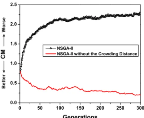
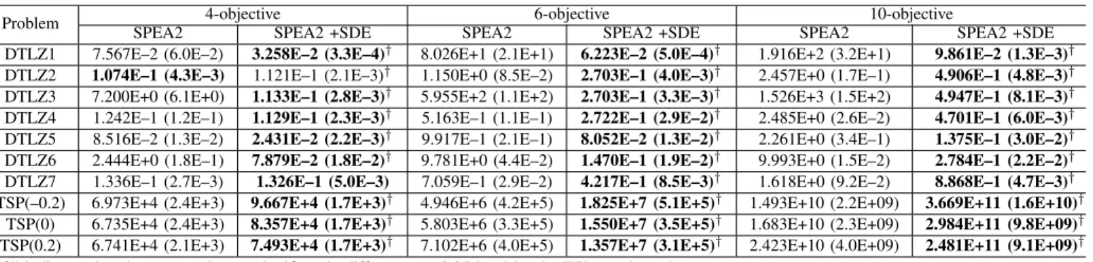
Fig. 1. Evolutionary trajectories of the convergence metric (CM) for a run of the original NSGA-II and the modified NSGA-II without the density estimation procedure on the 10-objective DTLZ2.

implementation of D(), as stated above, depends on the density estimator used in an EMO algorithm.

In Pareto-based EMO algorithms, in general, when two individuals are nondominated individuals in a population, the one with the lower density is preferable. This rule is very effective for an MOP with 2 or 3 objectives since it can provide a good balance between convergence and diversity. However, in many-objective optimization, this rule may fail to guide the population to search towards the optimal direction.

As mentioned before, the proportion of nondominated indi-viduals in the population becomes considerably large when a large number of objectives are involved. Extremely, all individuals in the population may become nondominated with each other. In this case, the density of individuals will play a leading or even unique role in distinguishing them in the selection process of algorithms. As a result, individuals that are distributed in sparse regions (i.e., individuals that have a low similarity degree to other individuals) will be preferred as long as they are nondominated in the population. However, it is likely that such individuals are located far away from the optimal front (e.g., they are slightly better than or comparable with other individuals in some objectives but are significantly worse in at least one objective). For example, considering a population of four nondominated individuals A,B,C, andD with their objective value(0,1,1,100),(1,0,2,1),(2,1,0,1), and (1,2,1,0), individual A performs the worst regarding convergence but is preferable in Pareto-based algorithms.

This density-leading criterion severely deteriorates the search performance of algorithms, which is reflected in both the mating and environmental selection. In the mating se-lection, there will be a higher probability that those poorly-converged nondominated individuals (such as individualAin the above example) are selected to recombine and produce low performance offspring. In the environmental selection, the long-term existence of those poorly-converged individuals will lead to the elimination of some well-converged ones due to the restriction of the population size. Consequently, the solutions, at the end of the optimization process, may be distributed widely over the objective space, but far away from the desired Pareto front. Figure 1 plots the evolutionary trajectories of the

(4)

convergence results2 _{of the original NSGA-II and its modified}

version where the density estimation procedure is removed for the 10-objective DTLZ2 [20]. Evidently, with the evolution process, the original NSGA-II gradually draws the population away from the Pareto front, while the removal of the crowding distance-based selection (used to distinguish individuals that are nondominated to each other) from NSGA-II noticeably improves the convergence performance of the algorithm.

The above observations indicate that the failure of Pareto-based EMO algorithms in many-objective optimization is due to their dislike for individuals in crowded regions. Then, can we “put” those poorly-converged individuals into crowded regions? In this case, any density estimator can identify these poorly-converged individuals as long as it can correctly reflect the crowding degree of individuals. Keeping this in mind, we present a new general density estimation methodology— shift-based density estimation (SDE); to facilitate contrast, we abbreviate the traditional density estimation as TDE.

B. Shift-based Density Estimation (SDE)

As stated previously, the density estimation of an individual in the population is based on the relative positions of other in-dividuals with regard to the individual. In SDE, we adjust these positions, trying to reflect the convergence of the individual in the population.

When estimating the density of an individualp, SDE shifts the positions of other individuals in the population according to the convergence comparison between these individuals and p on each objective. More specifically, if an individual performs better3 _than_p_{for an objective, it will be shifted to}

the same position ofpon this objective; otherwise, it remains unchanged. Formally, without lose of generality, assuming that we consider a minimization MOP, the new densityD′(p, P)of individual pin the populationP can be expressed as follows:

D′(p, P) =D(dist(p, q₁′), dist(p, q′₂), ..., dist(p, q′_N₋₁))

(2) where N denotes the size of P, dist(p, q′_i) is the similarity degree between individuals p and q′_i, and q′_i is the shifted version of individualqi(qi∈P andqi ̸=p), which is defined

as follows: q′_i₍_j₎= { p(j), if qi(j)< pi(j) qi(j), otherwise , j∈(1,2, ..., m) (3) where p(j), qi(j), and qi′(j) denote the j-th objective value

of individuals p, qi, and q′i, respectively, and m denotes the

number of objectives.

Figure 2 shows a bi-objective example to illustrate this shift-based density estimation operation. To estimate the density of individual Ain a population composed of four nondominated individuals A(10,17), B(1,18),C(11,6), and D(18,2), B is shifted to B′(10,18) since B1 = 1 < A1 = 10, and C and

2_{The results are evaluated by the convergence measure (CM) metric [18].}

CM assesses the convergence of a solution set by calculating the average normalized Euclidean distance from the set to the Pareto front.

3_{For minimization MOPs, performing better means having a lower value;}

for maximization MOPs, it means having a higher value.

Fig. 2. An illustration of shift-based density estimation in a bi-objective minimization scenario. To estimate the density of individualA, individualsB,

C, andDare shifted toB′,C′, andD′, respectively.

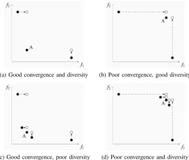
(a) Good convergence and diversity (b) Poor convergence, good diversity

(c) Good convergence, poor diversity (d) Poor convergence and diversity Fig. 3. Shift-based density estimation for four situations of an individual (A) in the population for a minimization MOP.

Dare shifted toC′(11,17)andD′(18,17), respectively, since C2= 6<A2= 17andD2= 2<A2= 17.

Clearly, individual A, which has a low similarity degree with other individuals in the original population, has two close neighbors in its new density estimation, and thus will be assigned a high density value. This occurs because there are two individuals B and C performing significantly better than A in terms of convergence (i.e., being slightly inferior to A in one or some objectives but greatly superior to A in the others). These individuals contribute large similarity degrees toAin its density estimation since the value on their advantageous objective(s) becomes equal to that of A. This means that the individuals which have no clear advantage over other individuals in the population will have a high density value in SDE.

In order to further understand SDE, we next consider four typical situations of the distribution of an individual in the population for a minimum MOP (i.e., performing well in convergence and diversity, performing well in diversity but poorly in convergence, performing well in convergence but poorly in diversity, and performing poorly in both convergence and diversity) in Fig. 3.

(5)

(a) Crowding Distance (b)k-th Nearest Neighbor (c) Grid Crowding Degree

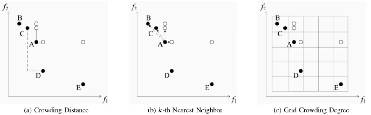
Fig. 4. An illustration of the three density estimators in traditional and shift-based density estimation, where individualAis to be estimated in the population.

good convergence and good diversity has a low crowding degree in SDE. The individual with either poor convergence or poor diversity has some close neighbors, and the individual with both poor convergence and poor diversity has the highest crowding degree in the four situations. In addition, note that the individuals with poor diversity (e.g., see Fig. 3(c) and Fig. 3(d)) are always located in crowded regions no matter how well they perform in terms of convergence, which means that SDE can maintain the distribution characteristic of in-dividuals in the population while reflecting the convergence difference between individuals.

C. Integrating SDE into NSGA-II, SPEA2, and PESA-II

In this section, we apply SDE to three classical Pareto-based EMO algorithms: NSGA-II [13], SPEA2 [81], and PESA-II [11]. NSGA-II is known for its nondominated sorting and crowding distance-based fitness assignment strategies. SPEA2 defines a strength value for each individual, and combines it with the k-th nearest neighbor method to distinguish individ-uals in the population. The main characteristic of PESA-II is its grid-based diversity maintenance mechanism, which is used in both the mating and environmental selection schemes. The density estimators (i.e., the crowding distance, k-th nearest neighbor, and grid crowding degree) in the three algorithms are representative and are briefly described below.

To estimate the density of an individual in the population, NSGA-II considers its two closest points on either side along each objective. The crowding distance is defined as the average distance between the two points on each objective. The nearest neighbor technique used in SPEA2 takes the distance of an individual to itsk-th nearest neighbor into account to estimate the density in its neighborhood. This density estimator is used in both the fitness assignment and archive truncation procedures to maintain diversity. PESA-II uses an adaptive grid technique to define the neighborhood of individuals. The density around an individual is estimated by the number of individuals in its hyperbox in the grid. Figure 4 illustrates the three density estimators used in TDE and SDE.

It is necessary to point out that since the crowding distance mechanism in NSGA-II separately estimates an individual’s crowding degree on each objective, individuals may be over-lapping on a single axis of the objective space in SDE. For example, when estimating the shift-based crowding degree of A on the f1 axis in Fig. 4(a), individuals A, B, and

C are overlapping. Here, we keep the original order before individuals are shifted. That is, on the f1 axis, individual C is still viewed as the left neighbor of A, and individual D is viewed as its right neighbor in the shift-based crowding distance calculation ofA. In this case, the crowding distance of A in TDE (shown with a dashed line) is changed to the average distance betweenAand the shifted CandDin SDE (shown with a solid line).

In Fig. 4(b), C and B are the two nearest neighbors of A in the original population (shown with a dashed arrow), but, to estimate the density of A in SDE, the two nearest individuals, the shifted DandC, are considered (shown with a solid arrow). Concerning Fig. 4(c), there is no individual in the neighborhood ofAin TDE, but in SDE, the shiftedD is the neighbor of A, thereby contributing to its grid crowding degree.

Overall, although the implementation of the three density estimators is totally different, the individuals (like individual D in Fig. 4) which do not perform significantly worse than the considered individual will contribute a lot to its density estimation in SDE.

In the next two sections, we will empirically investigate the proposed method, trying to answer the following questions— Can SDE improve the performance of all the three Pareto-based algorithms? Among these three density estimators, which one is the most suitable for SDE in many-objective optimization? How would the Pareto-based algorithms, when integrated with SDE, compare with other state-of-the-art algo-rithms designed specially for many-objective problems?

III. PERFORMANCEVERIFICATION OFSDE In this section, we validate SDE by integrating it to the aforementioned three Pareto-based algorithms, which re-sults in three new EMO algorithms, denoted NSGA-II+SDE, SPEA2+SDE, and PESA-II+SDE, respectively. We first sep-arately compare the three new algorithms with their corre-sponding original version. Thereafter, we put them together to further compare them and investigate the reason for their behavior in many-objective optimization.

Two well-defined test problem suites, the DTLZ [20] and the multiobjective travelling salesman problem (TSP) [12], are selected in this study. DTLZ is a continuous problem suite that can be scaled to any number of objectives and decision variables, commonly used in many-objective optimization.

(6)

TABLE I

PROPERTIES OF TEST PROBLEMS AND PARAMETER SETTING INPESA-II, PESA-II+SDE,ANDϵ-MOEA. THE SETTINGS OFdivANDϵCORRESPOND TO THE DIFFERENT NUMBERS OF OBJECTIVES OF A PROBLEM.MANDNDENOTE THE NUMBER OF OBJECTIVES AND DECISION VARIABLES,RESPECTIVELY

Problem M N Properties divin PESA-II divin PESA-II+SDE ϵinϵ-MOEA

DTLZ1 4, 6, 10 M+4 Linear, Multimodal 5, 40, 20 15, 12, 7 0.04, 0.054, 0.052

DTLZ2 4, 6, 10 M+9 Concave 5, 6, 7 11, 6, 4 0.105, 0.2, 0.275

DTLZ3 4, 6, 10 M+9 Concave, Multimodal 40, 40, 40 18, 16, 6 0.105, 0.2, 0.8

DTLZ4 4, 6, 10 M+9 Concave, Biased 6, 7, 10 13, 5, 4 0.105, 0.2, 0.275

DTLZ5 4, 6, 10 M+9 Concave, Degenerate 11, 7, 5 30, 20, 10 0.032, 0.11, 0.14

DTLZ6 4, 6, 10 M+9 Concave, Degenerate, Biased 9, 6, 6 23, 11, 5 0.095, 0.732, 1.48

DTLZ7 4, 6, 10 M+19 Mixed, Disconnected, Multimodal 7, 5, 3 13, 11, 5 0.09, 0.26, 0.73

TSP(–0.2) 4, 6, 10 30 Convex, Negative correlation 9, 6, 4 17, 9, 5 0.9, 1.9, 4.3

TSP(0) 4, 6, 10 30 Convex, Zero correlation 9, 5, 7 18, 10, 5 0.65, 1.3, 3.15

TSP(0.2) 4, 6, 10 30 Convex, Positive correlation 8, 5, 3 19, 10, 5 0.42, 0.85, 2.26

Consisting of problems with various characteristics (such as having linear, concave, nonconcave, multimodal, disconnected, biased, and degenerate Pareto fronts), the DTLZ suite is used to challenge different abilities of an algorithm. A detailed description of the DTLZ suite can be found in [20]

The multiobjective TSP is a typical combinatorial optimiza-tion problem and can be stated as follows [12]: given a network

L= (V, C), where V ={v1, v2, ..., vN} is a set of N nodes

andC={ck:k∈ {1,2, ..., M}}is a set ofM cost matrices

between nodes(ck:V ×V), we need to determine the Pareto

optimal set of Hamiltonian cycles that minimize each of the

M cost objectives. TheM matrices, according to [12], can be constructed as follows.

The matrix c1 is first generated by assigning each distinct pair of nodes with a random number between 0 and 1. Then the matrix ck+1 is generated according to the matrix ck:

ck+1(i, j) =T SP cp×ck(i, j) + (1−T SP cp)×rand (4)

whereck(i, j)denotes the cost from nodeito nodejin matrix

ck,randis a function to generate a uniform random number

in [0,1], andT SP cp ∈(−1,1) is a simple TSP “correlation parameter”. WhenT SP cp <0,T SP cp= 0, orT SP cp >0, it introduces negative, zero, or positive inter-objective correla-tions, respectively. In our study, T SP cp is assigned to−0.2,

0, and0.2to represent different characteristics of the problem. The characteristics of all the tested problems are summarized in Table I.

To compare the performance of the tested algorithms, the inverted generational distance (IGD) metric [6], [79] is selected since it can provide a combined information about convergence and diversity of a solution set. IGD measures the average distance from the points in the Pareto front to their closest solution in the obtained set. Mathematically, let P∗

be a reference set representing the Pareto front, and the IGD value from P∗ to the obtained solution setP is defined as:

IGD(P) = ∑

z∈P∗

d(z, P)

/

|P∗| (5)

where|P∗|denotes the size ofP∗ (i.e., the number of points inP∗) andd(z, P)is the minimum Euclidean distance fromz

toP. A low IGD value is preferable, which indicates that the obtained solution set is close to the Pareto front as well as has a good distribution. In the calculation of IGD, the knowledge of the Pareto front of a test problem is required. Here,

IGD is used to evaluate algorithms on the DTLZ problems since their optimal fronts are known. For the problem whose Pareto front is unknown (i.e., the multiobjective TSP), another comprehensive performance metric, hypervolume (HV) [82], is considered.

The HV metric is a very popular quality metric due to its good properties. HV calculates the volume of the objective space between the obtained solution set and a reference point, and a larger value is preferable. In the calculation of HV, a crucial issue is the choice of the reference point. Choosing a reference point that is slightly larger than the worst value of each objective on the Pareto front has been found to be suitable since the effects of convergence and diversity of the set can be well balanced [3], [42]. Since the range of the Pareto front is unknown in TSP, we regard the point with 22 for each objective (i.e.,r= 22M_{) as the reference point, given}

that it is slightly larger than the worst value of the mixed nondominated solution set constructed by all the obtained solution sets. In addition, since the exact calculation of the HV metric is infeasible for a solution set with 10 objectives, we approximately estimate the HV result of a solution set by the Monte Carlo sampling method used in [4]. Here, 107

sampling points are used to ensure accuracy [4].

The algorithm PESA-II requires a grid division parameter (div). Due to the integration of SDE, the optimal setting for

div in PESA-II+SDE is different from that in PESA-II. The settings ofdiv in Table I can enable the two algorithms sep-arately to achieve the best performance on the test instances. All the results presented in this paper are obtained by executing 30 independent runs of each algorithm on each problem with the termination criterion of 100,000 evaluations. Following the practice in [42], the population size was set to 200 for the tested algorithms, and the archive was also maintained with the same size if required. A crossover proba-bilitypc = 1.0 and a mutation probabilitypm= 1/N (where

N denotes the number of decision variables) were used. For the continuous problem DTLZ, the simulated binary crossover (SBX) and polynomial mutation with both distribution indexes 20 [16] were used as crossover and mutation operators. For the combinatorial TSP, the order crossover (OX) and inversion mutation were used according to [63].

A. NSGA-II vs NSGA-II+SDE

Table II shows the results of the two algorithms on the DTLZ and TSP problems regarding the mean and standard

(7)

TABLE II

PERFORMANCE COMPARISON BETWEENNSGA-IIANDNSGA-II+SDEREGARDING THE MEAN AND STANDARD DEVIATION(SD)VALUES ON THE

DTLZANDTSPTEST SUITES,WHEREIGDWAS USED FORDTLZANDHVFORTSP. THE BETTER RESULT REGARDING THE MEAN FOR EACH PROBLEM INSTANCE IS HIGHLIGHTED IN BOLDFACE

Problem _NSGA-II 4-objective_NSGA-II+SDE _NSGA-II 6-objective_NSGA-II+SDE _NSGA-II 10-objective_NSGA-II+SDE

DTLZ1 8.894E–2 (6.6E–2) 5.294E–2 (6.9E–3)† 2.141E+1 (1.9E+1) 1.512E+1 (7.8E+0) 4.471E+1 (3.3E+1) 4.801E+1 (2.2E+1)

DTLZ2 1.199E–1 (5.0E–3) 1.168E–1 (4.2E–3)† 1.104E+0 (1.7E–1) 6.160E–1 (8.0E–2)† 2.112E+0 (1.5E–1) 1.907E+0 (1.8E–1)†

DTLZ3 5.099E+0 (2.8E+0) 4.234E+0 (2.2E+0) 2.668E+2 (9.1E+1) 1.593E+2 (3.9E+1)† 5.928E+2 (1.9E+2) 3.802E+2 (1.4E+2)†

DTLZ4 1.096E–1 (3.6E–3) 1.098E–1 (3.1E–3) 7.038E–1 (1.8E–1) 3.388E–1 (3.9E–2)† 2.357E+0 (1.8E–1) 2.275E+0 (2.9E–2)†

DTLZ5 2.964E–2 (5.1E–3) 3.650E–2 (1.0E–2)† 1.030E–1 (3.6E–2) 1.503E–1 (3.4E–2)† 1.887E–1 (1.0E–1) 3.880E–1 (1.7E–1)†

DTLZ6 3.367E+0 (1.9E–1) 2.867E+0 (2.4E–1)† 8.346E+0 (3.7E–1) 7.772E+0 (4.5E–1)† 9.407E+0 (3.0E–1) 9.701E+0 (2.8E–1)†

DTLZ7 1.626E–1 (6.1E–3) 1.493E–1 (4.7E–3)† 5.676E–1 (1.7E–2) 5.227E–1 (1.9E–2)† 2.288E+0 (6.1E–1) 2.160E+0 (5.6E–1)

TSP(–0.2) 4.786E+4 (2.2E+3) 6.377E+4 (4.4E+3)† 2.861E+6 (4.7E+5) 4.274E+6 (5.2E+5)† 1.040E+10 (1.8E+09) 1.582E+10 (2.3E+09)†

TSP(0) 5.488E+4 (3.4E+3) 6.866E+4 (3.9E+3)† 4.041E+6 (4.4E+5) 5.669E+6 (6.0E+5)† 1.801E+10 (2.6E+09) 2.496E+10 (6.4E+09)†

TSP(0.2) 6.162E+4 (3.1E+3) 6.917E+4 (2.4E+3)† 5.379E+6 (7.0E+5) 7.580E+6 (8.0E+5)† 2.545E+10 (4.5E+09) 3.622E+10 (8.5E+09)†

“†” indicates that the two results are significantly different at a 0.05 level by the Wilcoxon’s rank sum test.

0 1 2 3 4 0 1 2 3 4 f1 f 2 NSGA-II NSGA-II+SDE

Fig. 5. Result comparison between NSGA-II and NSGA-II+SDE on the 10-objective DTLZ2. The final solutions of the algorithms are shown regarding the two-dimensional objective spacef1andf2.

deviation (SD) values, where IGD and HV were used for the DTLZ and TSP problems, respectively. The better result re-garding the mean for each problem is highlighted in boldface. Moreover, in order to have statistically sound conclusions, the Wilcoxon’s rank sum test [83] at a 0.05 significance level was adopted to test the significance of the differences between assessment results obtained by two competing algorithms.

As can be seen from Table II, the performance of NSGA-II has a clear improvement when SDE is applied to the algorithm, achieving a better value in 24 out of all 30 test instances. Also, for most of the problems on which NSGA-II+SDE outperforms NSGA-II, the results have statistical significance (21 out of the 24 problems). Especially, for the TSP problem suite, NSGA-II+SDE shows a significant advantage over its competitor, with statistical significance for all 9 test instances. Despite a clear improvement obtained, NSGA-II+SDE actu-ally struggles to cope with many-objective optimization prob-lems. Figure 5 plots the final solutions of the two algorithms in a single run regarding the two-dimensional objective space

f1 and f2 of the 10-objective DTLZ2. Similar plots can be obtained for other objectives of the problem. This particular run is associated with the result which is the closest to the mean IGD value. Clearly, although NSGA-II+SDE tends to perform slightly better than NSGA-II in terms of diversity, both algorithms fail to approach the Pareto front of the

4 8 12 16 20 24 4 8 12 16 20 24 SPEA2 SPEA2+SDE f 2 f1

Fig. 6. Result comparison between SPEA2 and SPEA2+SDE on the 10-objective TSP withT SP cp= 0. The final solutions of the algorithms are shown regarding the two-dimensional objective spacef1 andf2.

problem, given that the range of the optimal front is (0,1)

for each objective. A detailed explanation of the failure of NSGA-II+SDE will be given in Sect. III-D.

B. SPEA2 vs SPEA2+SDE

Table III shows the comparative results of the two algo-rithms on the DTLZ and TSP test problems. In contrast to the slight difference between NSGA-II+SDE and NSGA-II, SPEA2+SDE significantly outperforms the original SPEA2. SPEA2+SDE achieves a better value for all the 30 test instances except the 4-objective DTLZ2, and with statistical significance on 28 instances. Moreover, the advantage of SPEA2+SDE becomes clearer as the number of objectives increases—more than an order of magnitude advantage of IGD is obtained for most of the 10-objective instances (i.e., DTLZ1, DTLZ3, DTLZ5, DTLZ6, and three TSP problems with different conflict degrees among the objectives). Figure 6 shows the final solutions of a single run of SPEA2 and SPEA2+SDE regarding the objective space f1 andf2 of the 10-objective TSP withT SP cp= 0. It is clear from the figure that the convergence performance of SPEA2 is significantly improved when SDE is applied to the algorithm.

(8)

TABLE III

PERFORMANCE COMPARISON BETWEENSPEA2ANDSPEA2+SDEREGARDING THE MEAN AND STANDARD DEVIATION(SD)VALUES ON THEDTLZ

ANDTSPTEST SUITES,WHEREIGDWAS USED FORDTLZANDHVFORTSP. THE BETTER RESULT REGARDING THE MEAN FOR EACH PROBLEM INSTANCE IS HIGHLIGHTED IN BOLDFACE

Problem _SPEA2 4-objective_{SPEA2 +SDE} _SPEA2 6-objective_{SPEA2 +SDE} _SPEA2 10-objective_{SPEA2 +SDE}

DTLZ1 7.567E–2 (6.0E–2) 3.258E–2 (3.3E–4)† 8.026E+1 (2.1E+1) 6.223E–2 (5.0E–4)† 1.916E+2 (3.2E+1) 9.861E–2 (1.3E–3)†

DTLZ2 1.074E–1 (4.3E–3) 1.121E–1 (2.1E–3)† 1.150E+0 (8.5E–2) 2.703E–1 (4.0E–3)† 2.457E+0 (1.7E–1) 4.906E–1 (4.8E–3)†

DTLZ3 7.200E+0 (6.1E+0) 1.133E–1 (2.8E–3)† 5.955E+2 (1.1E+2) 2.703E–1 (3.3E–3)† 1.526E+3 (1.5E+2) 4.947E–1 (8.1E–3)†

DTLZ4 1.242E–1 (1.2E–1) 1.129E–1 (2.3E–3)† 5.163E–1 (1.1E–1) 2.722E–1 (2.9E–2)† 2.485E+0 (2.6E–2) 4.701E–1 (6.0E–3)†

DTLZ5 8.516E–2 (1.3E–2) 2.431E–2 (2.2E–3)† 9.917E–1 (2.1E–1) 8.052E–2 (1.3E–2)† 2.261E+0 (3.4E–1) 1.375E–1 (3.0E–2)†

DTLZ6 2.444E+0 (1.8E–1) 7.879E–2 (1.8E–2)† 9.781E+0 (4.4E–2) 1.470E–1 (1.9E–2)† 9.993E+0 (1.5E–2) 2.784E–1 (2.2E–2)†

DTLZ7 1.336E–1 (2.7E–3) 1.326E–1 (5.0E–3) 7.059E–1 (2.9E–2) 4.217E–1 (8.5E–3)† 1.618E+0 (9.2E–2) 8.868E–1 (4.7E–3)†

“†” indicates that the two results are significantly different at a 0.05 level by the Wilcoxon’s rank sum test. TABLE IV

PERFORMANCE COMPARISON BETWEENPESA-IIANDPESA-II+SDEREGARDING THE MEAN AND STANDARD DEVIATION(SD)VALUES ON THEDTLZ

ANDTSPTEST SUITES,WHEREIGDWAS USED FORDTLZANDHVFORTSP. THE BETTER RESULT REGARDING THE MEAN FOR EACH PROBLEM INSTANCE IS HIGHLIGHTED IN BOLDFACE

Problem 4-objective 6-objective 10-objective

PESA-II PESA-II+SDE PESA-II PESA-II+SDE PESA-II PESA-II+SDE

DTLZ1 5.740E–1 (4.5E–1) 3.729E–2 (3.4E–3)† 1.341E+1 (5.5E+0) 8.920E–2 (1.1E–2)† 2.802E+1 (8.7E+0) 1.552E–1 (4.4E–2)†

DTLZ2 1.227E–1 (6.9E–3) 1.113E–1 (5.3E–3)† 2.857E–1 (1.1E–2) 2.249E–1 (3.5E–3)† 5.671E–1 (3.1E–2) 3.756E–1 (3.2E–3)†

DTLZ3 7.593E+0 (4.4E+0) 2.365E–1 (2.5E–1)† 1.303E+2 (3.8E+1) 4.464E–1 (2.9E–1)† 3.037E+2 (5.3E+1) 1.222E+0 (1.4E+0)†

DTLZ4 1.192E–1 (7.8E–3) 2.752E–1 (2.8E–1) 2.969E–1 (6.2E–3) 2.579E–1 (6.4E–2)† 6.929E–1 (4.3E–2) 3.955E–1 (1.8E–2)†

DTLZ5 1.008E–1 (1.5E–2) 4.805E–2 (6.5E–3)† 3.599E–1 (6.3E–2) 3.283E–1 (7.4E–2) 5.202E–1 (1.1E–1) 4.087E–1 (7.0E–2)†

DTLZ6 1.797E+0 (1.1E–1) 1.510E–1 (2.7E–2)† 6.689E+0 (2.4E–1) 5.516E–1 (3.2E–2)† 8.690E+0 (3.7E–1) 8.679E–1 (1.2E–1)†

DTLZ7 1.415E–1 (6.5E–3) 1.352E–1 (4.8E–3)† 6.164E–1 (6.5E–2) 4.147E–1 (6.9E–2)† 7.522E+0 (1.7E+0) 1.259E+0 (3.6E–1)†

“†” indicates that the two results are significantly different at a 0.05 level by the Wilcoxon’s rank sum test.

C. PESA-II vs PESA-II+SDE

Using a grid technique to maintain diversity, PESA-II has been found to outperform NSGA-II and SPEA2 in many-objective optimization [46]. In spite of this, SDE can signif-icantly enhance the performance of PESA-II. Table IV gives the comparative results of PESA-II and PESA-II+SDE on the DTLZ and TSP test problems. PESA-II+SDE achieves a better assessment result than the original PESA-II on all the 30 instances except the 4-objective DTLZ4, and with statistical significance for 28 instances. Especially, on some MOPs where big obstacles exist for an algorithm to converge into the Pareto front, such as DTLZ1, DTLZ3, and DTLZ6, more than an order of magnitude advantage is achieved for all the 4, 6, and 10-objective instances. Figure 7 plots the final solutions of a single run of the two algorithms regarding the objective space

f1 andf2 of the 10-objective DTLZ6. A clear difference in terms of convergence between the two solution sets can be observed in the figure.

D. Comparison among NSGA-II+SDE, SPEA2+SDE, and PESA-II+SDE

Previous studies presented different behaviors of the three Pareto-based algorithms when SDE is integrated to them in many-objective optimization. This section compares the three new algorithms and tries to investigate: 1) why they behave differently, and 2) which density estimator is more suitable

0 1 2 3 4 5 6 0 1 2 3 4 f 2 f1 PESA-II PESA-II+SDE

Fig. 7. Result comparison between PESA-II and PESA-II+SDE on the 10-objective DTLZ6. The final solutions of the algorithms are shown regarding the two-dimensional objective spacef1andf2.

for SDE. Table V gives the comparative results of the three algorithms on the DTLZ and TSP test problems.

As can be seen from Table V, SPEA2+SDE and PESA-II+SDE significantly outperforms NSGA-II+SDE. SPEA2+SDE outperforms NSGA-II+SDE for all test instances except for the 4-objective DTLZ4, and PESA-II outperforms NSGA-II+SDE in 26 out of all 30 instances. Especially, for the 6- and 10-objective DTLZ1 and DTLZ3 problems, the advantage of the first two algorithms over NSGA-II+SDE is more than two orders of magnitude. On

(9)

TABLE V

PERFORMANCE COMPARISON(MEAN ANDSD)OFNSGA-II+SDE,

SPEA2+SDE,ANDPESA-II+SDEON THEDTLZANDTSPTEST

SUITES,WHEREIGDWAS USED FORDTLZANDHVFORTSP. THE BEST RESULT REGARDING THE MEAN VALUE AMONG THE THREE ALGORITHMS

FOR EACH PROBLEM INSTANCE IS HIGHLIGHTED IN BOLDFACE Problem Obj. NSGA-II+SDE SPEA2+SDE PESA-II+SDE DTLZ1

4 5.294E–2 (6.9E–2)† 3.258E–2 (3.3E–4)† 3.729E–2 (3.4E–3)† 6 1.512E+1 (7.8E+0)† 6.223E–2 (5.0E–4)† 8.920E–2 (1.1E–2)† 10 4.801E+1 (2.2E+1)† 9.861E–2 (1.3E–3)† 1.552E–1 (4.4E–2)† DTLZ2

4 1.168E–1 (4.2E–3)† 1.121E–1 (2.1E–3) 1.113E–1 (5.3E–3)†

6 6.160E–1 (8.0E–2)† 2.703E–1 (4.0E–3)† 2.249E–1 (3.5E–3)†

10 1.907E+0 (1.8E–1)† 4.906E–1 (4.8E–3)† 3.756E–1 (3.2E–3)†

DTLZ3

4 4.234E+0 (2.2E+0)† 1.133E–1 (2.8E–3)† 2.365E–1 (2.5E–1)† 6 1.593E+2 (3.9E+1)† 2.703E–1 (3.3E–3)† 4.464E–1 (2.9E–1)† 10 3.802E+2 (1.4E+2)† 4.947E–1 (8.1E–3)† 1.222E+0 (1.4E+0)† DTLZ4

4 1.098E–1 (3.1E–3)† 1.129E–1 (2.3E–3)† 2.752E–1 (2.8E–1) 6 3.388E–1 (3.9E–2)† 2.722E–1 (2.9E–2)† 2.579E–1 (6.4E–2)†

10 2.275E+0 (2.9E–2)† 4.701E–1 (6.0E–3)† 3.955E–1 (1.8E–2)†

DTLZ5

4 3.650E–2 (1.0E–2)† 2.431E–2 (2.2E–3)† 4.805E–2 (6.5E–3)† 6 1.503E–1 (3.4E–2)† 8.052E–2 (1.3E–2)† 3.283E–1 (7.4E–2)† 10 3.880E–1 (1.7E–1)† 1.375E–1 (3.0E–2)† 4.087E–1 (7.0E–2) DTLZ6

4 2.867E+0 (2.4E–1)† 7.879E–2 (1.8E–2)† 1.510E–1 (2.7E–2)† 6 7.772E+0 (4.5E–1)† 1.470E–1 (1.9E–2)† 5.516E–1 (3.2E–2)† 10 9.701E+0 (2.8E–1)† 2.784E–1 (2.2E–2)† 8.679E–1 (1.2E–1)† DTLZ7

4 1.493E–1 (4.7E–3)† 1.326E–1 (5.0E–3) 1.352E–1 (4.8E–3)† 6 5.227E–1 (1.9E–2)† 4.217E–1 (8.5E–3)† 4.147E–1 (6.9E–2)†

10 2.160E+0 (5.6E–1)† 8.868E–1 (4.7E–3)† 1.259E+0 (3.6E–1)† TSP(–0.2)

4 6.377E+4 (4.4E+3)† 9.667E+4 (1.7E+3)† 8.984E+4 (2.3E+3)† 6 4.274E+6 (5.2E+5)† 1.825E+7 (5.1E+5)† 1.533E+7 (6.4E+5)† 10 1.582E+10 (2.3E+09)†3.669E+11 (1.6E+10)†1.855E+11 (2.6E+10)† TSP(0)

4 6.866E+4 (3.9E+3)† 8.357E+4 (1.7E+3)† 7.883E+4 (1.8E+3)† 6 5.669E+6 (6.0E+5)† 1.550E+7 (3.5E+5)† 1.354E+7 (5.5E+5)† 10 2.496E+10 (6.4E+09)†2.984E+11 (9.8E+09)†2.022E+11 (1.5E+10)† TSP(0.2)

4 6.917E+4 (2.4E+3)† 7.493E+4 (1.7E+3)† 7.160E+4 (1.3E+3)† 6 7.580E+6 (8.0E+5)† 1.357E+7 (3.1E+5)† 1.249E+7 (3.8E+5)† 10 3.622E+10 (8.5E+09)†2.481E+11 (9.1E+09)†1.897E+11 (7.8E+09)† “†” indicates that the result of the considered algorithm is significantly different from that of its right algorithm (i.e., NSGA-II+SDE vs SPEA2+SDE, SPEA2+SDE vs PESA-II+SDE, and PESA-II+SDE vs NSGA-II+SDE) at a 0.05 level by the Wilcoxon’s rank sum test.

the other hand, considering the results between SPEA2+SDE and PESA-II+SDE, the performance difference is also clear. The former has an advantage over the latter in 24 out of the 30 instances. More specifically, SPEA2+SDE achieves better results on all the DTLZ1, DTLZ3, DTLZ5, DTLZ6, and TSP instances as well as on most of the DTLZ7 instances, while PESA-II+SDE performs better on the three instances of DTLZ2, 6- and 10-objective DTLZ4, and 6-objective DTLZ7. In addition, the difference among three algorithms has statistical significance on most of all the 30 test instances: 30 for NSGA-II+SDE versus SPEA2+SDE, 28 for SPEA2+SDE versus PESA-II+SDE, and 28 for PESA-II+SDE versus NSGA-II+SDE.

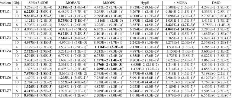
Figure 8 shows the final solutions of the three algorithms on the 10-objective DTLZ3 by parallel coordinates based on the single run where the result is the closest to the mean IGD value. The DTLZ3 test problem, by introducing a vast number of local optima (310₋₁_{), poses a stiff challenge for an}

algorithm to search towards the global optimal front, especially when the number of objectives becomes large. The global optimal front of the problem is a spherical front satisfying

f12+f22+...+fM2 = 1 in the range f1, f2, ..., fM ∈[0,1].

For this problem, NSGA-II+SDE fails to approach the Pareto front, with the upper boundary of its solutions exceeding 1600 on each objective, as shown in Fig. 8. Most of the solutions of

PESA-II+SDE can converge into the Pareto front, but fail to cover the whole optimal range. Only SPEA2+SDE can achieve a good balance between convergence and diversity, having a spread of solutions overfi∈[0,1]for all the 10 objectives.

Due to the ineffectiveness of the Pareto dominance re-lation in distinguishing individuals for many-objective opti-mization, the performance differences among NSGA-II+SDE, SPEA2+SDE, and PESA-II+SDE can be attributed to the dif-ferent behaviors of their density estimators (i.e., the crowding distance,k-th nearest neighbor, and grid crowding degree) in SDE. In the following, we will investigate them in detail.

Recall that to estimate the density of an individual, the crowding distance estimator considers its two closest points on either side along each objective. Due to this separate consideration of the neighbors on each objective, an incorrect estimation of an individual’s density may be obtained when the number of objectives is larger than two4_{. This phenomenon}

has been reported in Kukkonen and Deb’s study [52]. In this case, an individual which is far from other individuals in the population may be assigned a low (poor) crowding distance, leading to an incorrect estimation in SDE.

Consider a tri-objective scenario where a population is com-posed of four nondominated individualsA(1,1,1),B(0,10,2), C(2,0,10), and D(10,2,0), as shown in Fig. 9 by parallel coordinates. Clearly, individual A has a low similar degree with the other three individuals and performs significantly better than them in terms of convergence. However, A is assigned a poor crowding distance in both TDE and SDE. In TDE, A has two close neighbors on each objective (i.e., B and C on f1, C and D on f2, and D and B on f3). In SDE, the upper neighbor of A on each objective remains unchanged, while the lower neighbor moves to the position of A. Thus, the crowding distance of Ain SDE is CD(A) =

((Af1−Cf1) + (Af2−Df2) + (Af3−Bf3))/3 = 1, which is

clearly worse than CD(B) =CD(C) =CD(D) = 3. Unlike the crowding distance, the k-th nearest neighbor and grid crowding degree estimators consider an individual as a whole, thus avoiding the above misjudgment. The inferior performance of PESA-II+SDE against SPEA2+SDE may be due to the coarseness of the grid-based density estimator. As pointed out in [29], the judgement of density of an individual in grid depends partly on the size of a hyperbox and the position of the hyperbox where the individual is located.

As an explanation for the problem of the grid crowding de-gree, Fig. 10 shows a bi-objective nondominated set consisting of individualsA,B,C,D, andE. IndividualDperforms worse thanCandE in terms of convergence, thus having two very close neighbors G and H in SDE. However, since they are distributed in different hyperboxes, the grid crowding degree ofDis still equal to one. In contrast, individualC, which has a relatively distant neighbor F in its hyperbox, is assigned a higher grid crowding degree (2). Concerning thek-th nearest neighbor in SPEA2+SDE, it is clear thatDhas a higher density 4_{For a bi-objective problem, the crowding distance can correctly estimate}

the density of an individual in the nondominated set since the property of the Pareto dominance relation (which implies a monotonic relation between individuals in the objective space) causes individuals to come close together along both the objectives.

(10)

1 2 3 4 5 6 7 8 9 10 0 500 1000 1500 2000 Objective No. O b j e c t i v e V a l u e 1 2 3 4 5 6 7 8 9 10 0.0 0.2 0.4 0.6 0.8 1.0 Objective No. O b j e c t i v e V a l u e 1 2 3 4 5 6 7 8 9 10 0.0 0.5 1.0 1.5 2.0 O b j e c t i v e V a l u e Objective No.

(a) NSGA-II+SDE (b) SPEA2+SDE (c) PESA-II+SDE

Fig. 8. The final solution set of the three algorithms on the ten-objective DTLZ3, shown by parallel coordinates.

1 2 3 0 2 4 6 8 10 O b j e c t i v e V a l u e Objective No. A B C D

Fig. 9. An illustration of the failure of the crowding distance in TDE and SDE on a tri-objective scenario, showed by parallel coordinates. In a nondominated set consisting of A(1,1,1),B(0,10,2), C(2,0,10), and

D(10,2,0), individualAperforms well in terms of convergence and diversity. ButAwill be assigned a poor density value in both TDE and SDE since the crowding distance separately considers its neighbors on each objective.

Fig. 10. An illustration of the inaccuracy of the grid crowding degree.D

has two very close neighborsGandHin SDE, but its grid crowding degree is smaller than that ofCwhich has a relatively distant neighborF.

value than Csince the Euclidean distance between Dand its nearest neighbor G is smaller than that between C and its nearest neighborF.

Overall, the performance difference among the algorithms is due to the difference in the degree of accuracy of their density estimators. A density estimator will be well suitable in SDE as long as it can accurately estimate the density of individuals. In the next section, we will test the competitiveness of the proposed method to existing state-of-the-art methods in many-objective optimization by comparing SPEA2+SDE with five representative algorithms taken from different branches of

solving many-objective problems.

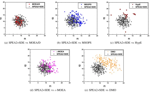
IV. COMPARISON WITHSTATE-OF-THE-ARTALGORITHMS

We consider the following five EMO algorithms to verify the proposed method.

• MOEA/D [79]. As a representative algorithm developed recently, MOEA/D is an aggregation-based algorithm. The high search ability of MOEA/D on both multi- and many-objective problems has already been demonstrated in the literature [37], [55]. Two aggregation functions, Tchebycheff and penalty-based boundary intersection (PBI), can be used in the algorithm, and each of them works well on different classes of problems. Here, the PBI function is selected since MOEA/D with PBI has been found to be more competitive when solving prob-lems with a high-dimensional objective space [16], [17]. • MSOPS[32]. MSOPS, based on converting a multiobjec-tive problem into a number of single-objecmultiobjec-tive problems by a predefined set of well-distributed weight vectors, also belongs to the class of aggregation-based approaches. Unlike MOEA/D where an individual corresponds to only one weight vector, MSOPS specifies an individual with a number of weight vectors. MSOPS is a popular algorithm to solve many-objective problems since it can achieve a good balance between convergence and diversity [71]. • HypE [4]. HypE is an indicator-based algorithm which

uses the hypervolume metric to guide the search for many-objective optimization. HypE adopts a Monte Carlo simulation to approximate the exact hypervolume value, significantly reducing the time cost of the HV calculation and enabling hypervolume-based search to be easily applied on many-objective optimization, even when the number of objectives reaches 50 [4].

• ϵ-MOEA[19].ϵ-MOEA is a steady-state algorithm using

ϵ-dominance to strengthen the selection pressure towards the Pareto front. Dividing the objective space into many hyperboxes, ϵ-MOEA assigns each hyperbox at most a single solution based on ϵ-dominance and the distance from solutions to the utopia point in the hyperbox. Although not specifically designed for many-objective optimization, ϵ-MOEA has been found to perform well on many-objective problems [28], [71].

• DMO[1]. Like SDE, DMO modifies the diversity main-tenance mechanism of Pareto-based algorithms to im-prove their performance for many-objective problems.

(11)

TABLE VI

IGDRESULTS(MEAN ANDSD)OF THE SIX ALGORITHMS ON THEDTLZPROBLEMS. THE BEST RESULT REGARDING THE MEANIGDVALUE AMONG THE ALGORITHMS FOR EACH PROBLEM INSTANCE IS HIGHLIGHTED IN BOLDFACE

Problem Obj. SPEA2+SDE MOEA/D MSOPS HypE ϵ-MOEA DMO

DTLZ1

4 3.258E–2 (3.3E–4) 3.218E–2 (1.0E–4)† 4.442E–2 (2.7E–3)† 8.728E–2 (9.6E–3)† 3.508E–2 (1.6E–3)† 4.249E–2 (1.8E–3)† 6 6.223E–2 (5.0E–4) 6.489E–2 (3.7E–4)† 3.263E–1 (3.8E–1)† 3.267E–1 (2.4E–1)† 9.504E–2 (1.1E–1)† 4.336E–1 (2.8E–1)† 10 9.861E–2 (1.3E–3) 1.017E–1 (1.6E–3)† 2.095E+0 (1.3E+0)† 4.000E–1 (1.7E–1)† 3.098E–1 (3.0E–1)† 2.709E+0 (3.8E+0)† DTLZ2

4 1.121E–1 (2.1E–3) 8.739E–2 (5.1E–6)† 1.116E–1 (2.5E–3) 1.873E–1 (2.6E–2)† 1.051E–1 (1.7E–3)† 1.415E–1 (1.7E–2)† 6 2.703E–1 (4.0E–3) 2.566E–1 (2.0E–5)† 3.228E–1 (9.2E–3)† 3.857E–1 (4.5E–2)† 2.429E–1 (3.7E–3)† 2.756E–1 (1.4E–2) 10 4.906E–1 (4.8E–3) 4.921E–1 (6.9E–5) 6.852E–1 (4.9E–2)† 6.294E–1 (9.4E–2)† 4.048E–1 (4.9E–3)† 5.280E–1 (1.8E–2)† DTLZ3

4 1.133E–1 (2.8E–3) 9.172E–2 (3.2E–3)† 2.101E+1 (1.1E+1)† 3.515E–1 (1.2E–1)† 1.172E–1 (5.5E–3)† 1.662E+0 (1.5E+0)† 6 2.703E–1 (3.3E–3) 2.616E–1 (8.6E–3)† 5.702E+1 (1.4E+1)† 1.783E+0 (1.2E+0)† 3.365E–1 (1.1E–1)† 5.076E+1 (1.5E+1)† 10 4.947E–1 (8.1E–3) 4.950E–1 (5.0E–3) 8.303E+1 (1.7E+1)† 2.242E+0 (1.3E+0)† 1.273E+1 (2.0E+1)† 2.368E+2 (8.2E+1)† DTLZ4

4 1.129E–1 (2.3E–3) 3.537E–1 (2.9E–1)† 1.116E–1 (3.2E–3) 2.130E–1 (1.3E–1)† 1.531E–1 (1.3E–1) 1.285E–1 (1.1E–2)† 6 2.722E–1 (2.9E–2) 5.231E–1 (1.2E–1)† 3.212E–1 (9.3E–3)† 4.887E–1 (5.5E–2)† 3.150E–1 (1.0E–1) 3.600E–1 (2.1E–2)† 10 4.701E–1 (6.0E–3) 6.778E–1 (7.0E–2)† 6.755E–1 (2.4E–2)† 8.358E–1 (7.6E–2)† 4.725E–1 (5.8E–2) 6.822E–1 (3.8E–2)† DTLZ5

4 2.431E–2 (2.2E–3) 1.607E–2 (1.8E–5)† 1.557E–2 (1.4E–3)† 9.803E–2 (1.8E–2)† 3.622E–2 (2.4E–3)† 3.062E–1 (5.5E–2)† 6 8.052E–2 (1.3E–2) 2.361E–2 (1.4E–4)† 1.476E–2 (1.8E–3)† 8.630E–2 (2.1E–2) 1.214E–1 (1.5E–2)† 4.510E–1 (1.0E–1)† 10 1.375E–1 (3.0E–2) 6.495E–2 (2.2E–6)† 1.769E–2 (2.0E–3)† 1.472E–1 (3.2E–2) 1.714E–1 (1.7E–2)† 4.656E–1 (1.1E–1)† DTLZ6

4 7.879E–2 (1.8E–2) 8.636E–2 (3.0E–2) 2.495E+0 (5.8E–1)† 3.473E+0 (5.0E–1)† 6.318E–1 (4.5E–2)† 7.198E+0 (2.2E–1)† 6 1.470E–1 (1.9E–2) 1.205E–1 (3.6E–2)† 7.788E+0 (3.0E–1)† 5.991E+0 (5.8E–1)† 2.904E+0 (2.4E–1)† 6.129E+0 (3.6E–1)† 10 2.784E–1 (2.2E–2) 1.532E–1 (4.0E–2)† 7.738E+0 (2.8E–1)† 5.573E+0 (4.4E–1)† 3.175E+0 (1.9E+0)† 7.769E+0 (4.2E–1)† DTLZ7

4 1.326E–1 (5.0E–3) 4.898E–1 (1.0E–1)† 4.873E–1 (1.2E–1)† 2.923E–1 (8.0E–3)† 2.189E–1 (9.9E–2)† 1.430E–1 (5.6E–3)† 6 4.217E–1 (8.5E–3) 3.923E+0 (9.2E–1)† 9.989E+0 (1.5E+0)† 6.246E–1 (9.7E–2)† 6.815E–1 (1.3E–1)† 5.505E–1 (2.5E–2)† 10 8.868E–1 (4.7E–3) 4.193E+0 (1.2E+0)† 2.208E+1 (3.0E+0)† 1.010E+0 (3.3E–2)† 1.879E+0 (1.8E–1)† 6.561E+0 (2.5E+0)† “†” indicates that the results of the peer algorithm is significantly different from that of SPEA2+SDE at a 0.05 level by the Wilcoxon’s rank sum test.

By comparing the boundary values between the current population and the Pareto front, DMO adaptively adjusts the diversity requirement in the mating and environmental selection schemes. If the range of the current population is smaller than that of the Pareto front of the problem by the Maximum Spread test [82], the diversity promotion mechanism is activated; otherwise, it is deactivated. Overall, the above peer algorithms are representative algo-rithms to address many-objective problems, and their perfor-mance has been well verified in many-objective optimization [26], [28], [57], [71], [72].

Parameters need to be set in some of the peer algorithms. According to their original papers, the neighborhood size and the penalty parameter in MOEA/D were set to 10% of the population size and 5, respectively, and the number of sampling points in HypE was set to 10,000. Since increasing the number of weight vectors with the number of objectives benefits the performance of MSOPS, 200 weight vectors were selected in MSOPS according to the experimental results in [71]. Inϵ-MOEA, the size of the archive set is determined by the ϵvalue. In order to guarantee a fair comparison, we setϵ

so that the archive of ϵ-MOEA is approximately of the same size (200) as that of the other algorithms (given in Table I). In addition, in MOEA/D the population size cannot be arbitrarily specified since it is equal to the number of weight vectors. As suggested in [42], we used the closest number to 200 among the possible values as the population size (i.e., 220, 252, and 220 for 4-, 6-, and 10-objective problems, respectively).

A. Comparison on the DTLZ Test Problems

Table VI shows the comparative results of the six algo-rithms on the DTLZ problem suite. First, we consider the DTLZ1 problem which has an easy, linear Pareto front but having a huge number of local optima (115 ₋₁_{). For this}

problem, SPEA2+SDE and MOEA/D perform clearly better than the other four algorithms. More precisely, MOEA/D slightly outperforms SPEA2+SDE on the 4-objective instance, while SPEA2+SDE achieves a lower IGD value when a larger number of objectives are involved.

Although having the same optimal front, the problems DTLZ2, DTLZ3, and DTLZ4 are designed to challenge dif-ferent capabilities of an algorithm. DTLZ2 is a relatively easy function with a spherical Pareto front. Based on DTLZ2, a vast number of local optima are introduced in DTLZ3, creating a big challenge for algorithms to search towards the global optimal front, and a non-uniform density of solutions are in-troduced in DTLZ4, creating a big challenge for algorithms to maintain diversity in the objective space. As can be seen from Table VI, for the DTLZ2 problem, generally, ϵ-MOEA per-forms the best, followed by MOEA/D and SPEA2+SDE. On DTLZ3, MOEA/D and SPEA2+SDE are significantly superior to the other algorithms. The former reaches the best result on the two low-dimensional instances, and the latter outperforms the other algorithms when the number of objectives reaches 10. On DTLZ4, SPEA2+SDE is very competitive. Although MSOPS performs slightly better than SPEA2+SDE on the 4-objective instance, SPEA2+SDE has a clear advantage over the other algorithms for the remaining instances. In addition, note that MOEA/D, which works very well on the first three problems (DTLZ1, DTLZ2, and DTLZ3), tends to struggle on DTLZ4, obtaining the worst IGD value on 4- and 6-objective test instances. Similar observations have been reported in [16]. The Pareto front of DTLZ5 and DTLZ6 is a degenerate curve in order to test the ability of an algorithm to find a lower-dimensional optimal front while working with a higher-dimensional objective space. The difference between the two problems is that DTLZ6 is much harder than DTLZ5 by intro-ducing bias in thegfunction [20]. For such problems, MSOPS and MOEA/D work very well. The former performs the best

(12)

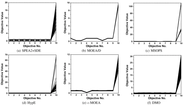
1 2 3 4 5 6 7 8 9 10 0 4 8 12 16 20 O b j e c t i v e V a l u e Objective No. 1 2 3 4 5 6 7 8 9 10 0 2 4 6 8 10 O b j e c t i v e V a l u e Objective No. 1 2 3 4 5 6 7 8 9 10 0 20 40 60 80 100 O b j e c t i v e V a l u e Objective No.

(a) SPEA2+SDE (b) MOEA/D (c) MSOPS

1 2 3 4 5 6 7 8 9 10 0 10 20 30 40 50 60 70 O b j e c t i v e V a l u e Objective No. 1 2 3 4 5 6 7 8 9 10 0 3 6 9 12 O b j e c t i v e V a l u e Objective No. 1 2 3 4 5 6 7 8 9 10 0 5 10 15 20 25 30 O b j e c t i v e V a l u e Objective No.

(d) HypE (e)ϵ-MOEA (f) DMO

Fig. 11. The final solution set of the six algorithms on the ten-objective DTLZ7, shown by parallel coordinates. TABLE VII

HVRESULTS(MEAN ANDSD)OF THE SIX ALGORITHMS ON THETSPPROBLEMS. THE BEST RESULT REGARDING THE MEANHVVALUE AMONG THE ALGORITHMS FOR EACH PROBLEM INSTANCE IS HIGHLIGHTED IN BOLDFACE

Problem Obj. SPEA2+SDE MOEA/D MSOPS HypE ϵ-MOEA DMO

TSP(–0.2)

4 9.667E+4 (1.7E+3) 9.394E+4 (1.7E+3)† 7.574E+4 (2.8E+3)† 3.817E+4 (4.5E+3)† 9.044E+4 (1.7E+3)† 5.224E+4 (3.1E+3)† 6 1.825E+7 (5.1E+5) 1.725E+7 (4.0E+5)† 1.061E+7 (6.5E+5)† 2.500E+6 (7.4E+5)† 1.428E+7 (6.6E+5)† 2.893E+6 (4.9E+5)† 103.669E+11 (1.6E+10)2.572E+11 (1.2E+10)†1.980E+11 (1.7E+10)† 1.033E+10 (1.2E+09)† 1.337E+11 (1.2E+10)†8.084E+09 (1.6E+09)† TSP(0)

4 8.357E+4 (1.7E+3) 8.358E+4 (1.4E+3) 6.779E+4 (2.0E+3)† 3.973E+4 (2.5E+3)† 7.935E+4 (2.1E+3)† 5.380E+4 (2.9E+3)† 6 1.550E+7 (3.5E+5) 1.458E+7 (3.3E+5)† 1.065E+7 (6.9E+5)† 3.930E+6 (4.8E+5)† 1.331E+7 (5.0E+5)† 3.965E+6 (4.9E+5)† 10 2.984E+11 (9.8E+09)1.969E+11 (1.3E+10)† 1.898E+11 (1.1E+10)†1.613E+10 (9.8E+08)† 1.440E+11 (9.3E+09)†1.691E+10 (3.2E+09)† TSP(0.2)

4 7.493E+4 (1.7E+3) 7.427E+4 (1.7+3) 6.210E+4 (1.6E+3)† 4.639E+4 (3.7E+3)† 7.230E+4 (1.9E+3)† 6.203E+4 (3.2E+3)† 6 1.357E+7 (3.1E+5) 1.264E+7 (3.1E+5)† 1.068E+7 (5.2E+5)† 5.468E+6 (5.3E+5)† 1.240E+7 (4.2E+5)† 5.355E+6 (7.6E+5)† 10 2.481E+11 (9.1E+09)1.580E+11 (1.0E+10)† 1.662E+11 (9.2E+09)†4.136E+10 (7.2E+09)† 1.530E+11 (1.3E+10)†2.504E+10 (5.2E+09)† “†” indicates that the results of the peer algorithm is significantly different from that of SPEA2+SDE at a 0.05 level by the Wilcoxon’s rank sum test.

on DTLZ5, and the latter outperforms the other algorithms on most of the DTLZ6 instances. Nevertheless, SPEA2+SDE show advantages in the low-dimensional DTLZ6, and for the high-dimensional instances, it performs significantly bet-ter than the peer algorithms except MOEA/D. On DTLZ5, SPEA2+SDE is always in the third place, better than HypE,

ϵ-MOEA, and DMO.

With a number of disconnected Pareto optimal regions, DTLZ7 tests an algorithm’s ability to maintain sub-populations in disconnected portions of the objective space. For this problem, SPEA2+SDE has a clear advantage over the other five algorithms, obtaining the best IGD value for all the three instances. In contrast, two aggregation-based algorithms, MOEA/D and MSOPS, have great difficulty with this problem. The former performs the worst on the 4-objective instance, and the latter obtains the worst IGD result for the 6- and 10-objective instances. Figure 11 plots the final solutions of the six algorithms in a single run on the 10-objective DTLZ7 by parallel coordinates. This particular run is associated with the result which is the closest to the mean IGD value. It is clear from Table VI that the solutions of MSOPS, HypE, and DMO fail to converge into the optimal front (the upper bound of the

last objective in the Pareto front of DTLZ7 is equal to2×M, i.e., f10 ≤ 20 for the 10-objective instance). MOEA/D and ϵ-MOEA struggle to maintain diversity, with their solutions converging into a portion of the disconnected Pareto front. Only SPEA2+SDE achieves a good approximation and cover-age of the Pareto front.

Overall, SPEA2+SDE is very competitive on the DTLZ problem suite. It obtains the best IGD value in 9 out of the 21 test instances, followed by MOEA/D, MSOPS, and

ϵ-MOEA, with the best value in 6, 4, and 2, respectively. Moreover, unlike MOEA/D and MSOPS, whose search ability has sharp contrasts on different problems, SPEA2+SDE has stable performance, ranking well for all the test instances.

B. Comparison on the TSP Test Problems

EMO algorithms ususally show different behavior on com-binatorial optimization problems than on continuous ones. One important property of the multiobjective TSP problem is that the conflict degree among the objectives can be adjusted according to the parameter T SP cp, where a lower value means a greater degree of conflict. From the HV results shown in Table VII, the advantage of SPEA2+SDE over the