Tamvakis, A., Anagnostopoulos, C.-N., Tsirtsis, G., Niros, A. D. and Spatharis, S.
(2018) Optimized classification predictions with a new index combining machine
learning algorithms. International Journal on Artificial Intelligence Tools, 27(3),
1850012.
There may be differences between this version and the published version. You are
advised to consult the publisher’s version if you wish to cite from it.
http://eprints.gla.ac.uk/163013/
Deposited on: 13 September 2018
Enlighten – Research publications by members of the University of Glasgow
Optimized classification predictions with a new index combining machine learning algorithms
Androniki Tamvakis
Department of Marine Sciences, University of the Aegean, University Hill, Mytilene, 81100, Greece
Christos-Nikolaos Anagnostopoulos
Department of Cultural Technology and Communication, University of the Aegean, University Hill, Mytilene, 81100, Greece
George Tsirtsis
Department of Marine Sciences, University of the Aegean, University Hill, Mytilene, 81100, Greece
Antonios D. Niros
Department of Cultural Technology and Communication, University of the Aegean, University Hill, Mytilene, 81100, Greece
Sofie Spatharis
Institute of Biodiversity, Animal Health and Comparative Medicine, University of Glasgow, Glasgow, Scotland, G12 8QQ, UK
Voting is a commonly used ensemble method aiming to optimize classification predictions by combining results from individual base classifiers. However, the selection of appropriate classifiers to participate in voting algorithm is currently an open issue. In this study we developed a novel Dissimilarity-Performance (DP) index which incorporates two important criteria for the selection of base classifiers to participate in voting: their differential response in classification (dissimilarity) when combined in triads and their individual performance. To develop this empirical index we firstly used a range of different datasets to evaluate the relationship between voting results and measures of dissimilarity among classifiers of different types (rules, trees, lazy classifiers, functions and Bayes). Secondly, we computed the combined effect on voting performance of classifiers with different individual performance and/or diverse results in the voting performance. Our DP index was able to rank the classifier combinations according to their voting performance and thus to suggest the optimal combination. The proposed index is recommended for individual machine learning users as a preliminary tool to identify which classifiers to combine in order to achieve more accurate classification predictions avoiding computer intensive and time-consuming search.
Keywords: voting ensemble method; classification; classifier dissimilarity; individual performance; classifier ensemble index.
1. Introduction
Machine Learning (ML) refers to the construction and study of algorithms that acquire information from collected data aiming to the most effective generalization and representation of the scientific issue under consideration.1 Classification is one of the most common ML applications, whereby an output variable (target class) with discrete and unordered values (labels) is predicted from a set of collected samples (instances) that consist the training set (dataset).2 This approach spans cutting edge applications over a wide variety of scientific fields 3,4 such as bioinformatics,5 medical science,6 computing,7 astronomy,8 engineering,9 remote sensing10,11 and environmental science.12
The increased interest in classification resulted in the development of numerous classifiers, differentiated in supervised or unsupervised depending on whether the training dataset is labeled a priori or not.13 Among the most popular supervised classifiers are decision trees, multilayer perceptron, naïve Bayes classifiers, instance based learning and support vector machines.14 Despite their wide variety, no optimal classifier has been established so far.15 Instead, the classification performance depends on the dataset properties (e.g. input variables, number of training samples)11,16 or the method used to assess classifier performance.17
Current research on ML focuses on integrating optimal classification results from multiple classifiers using specialized techniques called ensemble methods (EMs).18-20 These methods provide significantly improved classification performance compared to the base classifiers.18,19,21,22 Voting is a particularly useful and comprehensive EM that collects votes (i.e. predicted labels of the target class) from multiple classifiers and predicts the label of the target class yielding the highest value (expressed as number of votes or probability). Voting is the most widely applicable EM method, while other EMs (including bagging and boosting) are also based on voting to provide classification.23,24 Voting is the simplest and easiest way to combine classifiers,25-27 demanding no extra training for final prediction except for the pre-existing individual classifier classifications.28 Due to its ability to significantly improve predictions, voting spans many applications ranging from simple classification tasks29,30 to more complex implementations such as clustering,31 pairwise comparison32 and fuzzy systems.33,34 The challenging step when employing a voting algorithm is the selection of the base classifiers to be combined. When the number of potential classifier combinations and the size of the dataset are rather small, the optimal classifier combination can be determined exhaustively. However, this search becomes increasingly labor intensive and time consuming as the dataset and classifier complexity increase.35 To simplify this process, appropriate criteria must be applied for the selection of optimal classifiers to participate in the voting algorithm. For instance when classifiers in a voting scheme are highly dissimilar or independent (as assessed with dissimilarity indices), the classification performance may be significantly improved since the misclassification of one classifier can be potentially corrected by the success of another.36-39 Previous studies tried to incorporate the classifiers’ diversity in order to construct successful ensembles by using
different methods such as clustering, pruning, proper weighting based on various diversity measures, fuzzy logic, greedy search, particle swarm optimization, random sampling or data manipulation.19,20,23,26,40-43
Another important criterion is the performance of individual base classifiers to be combined during voting. Although it would seem intuitive to combine the best performing classifiers during voting, previous studies have shown that the best classification is not always achieved by combining classifiers that show the best individual performance.35,44,45 Therefore, the selection of the best combination of base classifiers should be based on simple and flexible criteria that will jointly consider their dissimilarity or independence along with their individual classification performance. 26,46-48
In this study we aim to develop a user-friendly index capable of identifying the optimal combination of base classifiers feeding into the voting algorithm and maximizing its classification performance. To this aim, the specific objectives are (a) to assess the efficiency of base classifiers in performing substantially different classification tasks, (b) to identify combinations of base classifiers that have markedly different behavior (i.e. high dissimilarity), (c) to test whether these combinations also have a corresponding high performance in voting classification, and (d) to develop a new user-friendly index that will incorporate the two criteria of classifier dissimilarity and individual performance, by assigning them appropriate weights. We expect that this dissimilarity-performance (DP) index will be more efficient in selecting the most appropriate base classifiers to be combined for voting than the traditionally applied dissimilarity indices. In order to subjectively evaluate its efficiency, DP will be confronted with substantially different classification tasks based on 28 (training and testing) datasets spanning different scientific fields.
2. Methods
2.1 Outline of the Methodology
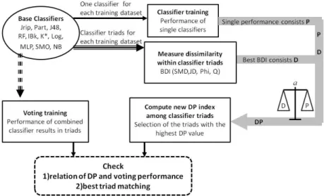
The development of the DP index, identifying the optimal combination of base classifiers to perform classification tasks, was carried out as follows (Fig. 1). Initially 10 base classifiers were trained in order to directly compare their individual performance in 14 different classification tasks (training datasets). This information was later used in the development of the new index which incorporates the individual performance of the base classifiers. The next step involved the training of the voting algorithm with all possible combinations of the 10 base classifiers in triads using all datasets. Thus, for each dataset the voting EM was trained using 120 different triads of base classifiers (denoted by all combinations of 3 out of the 10 selected base classifiers) and the voting performance of each triad was specified. Then, Binary Dissimilarity Indices (BDIs) were computed for all possible classifier triads of the training datasets to quantify within triad dissimilarity, and this measure was correlated with the corresponding voting performance. The last step
was the development of the new DP index that takes into account both the individual performance of each base classifier and the dissimilarity of classifiers within triads used in voting. These two characteristics were optimally weighted using a weighing parameter a for all training datasets. To check whether DP efficiently rates the classifier combinations according to their voting performance, the DP classification performance was correlated with the corresponding voting performance of triads across the 14 testing datasets. To test whether DP can identify the optimal classifier triad we checked whether the optimal triad based on voting performance was amongst those that DP identified as the best classifier combinations. Finally, the overall behavior of DP was examined across all testing datasets, to assess its efficiency and consistency to perform substantially different classification tasks.
Fig. 1. Schematic diagram of the methodological steps followed in the development and testing of the proposed Dissimilarity-Performance (DP) index. This index takes into account both the individual performance of base classifiers (P) and the dissimilarity (D) of classifier performance -measured with Binary Dissimilarity Indices (BDIs) - when those are combined in triads.
All base classifiers were trained with the WEKA machine learning package (version 3.6.9).49 This package was also used for training the voting algorithm with all possible combinations of classifiers in triads. The purpose of DP index is to identify the optimal combination of classifiers maximizing the classification performance during voting and therefore it is not necessary for base classifiers to participate with their highest potential performance. For this reason, the training of each classifier was performed using the default parameter values of the WEKA package.
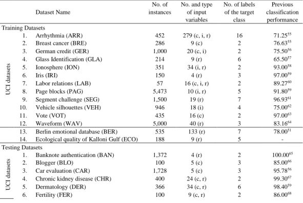
Twenty eight datasets (Table 1) were randomly split into two groups. The first group was used for the training of base classifiers and voting EM in order to determine the weight of the DP index parameter a (Fig. 1). Twelve datasets of the first group are available from the UCI machine learning repository and two are related with the research interests of the authors. The first of those is the Berlin Emotional (BER) database (EMO-DB),50 which contains 535 utterances of 10 actors (5 male, 5 female) predicting 7 emotional states (anger, happiness, anxiety/fear, sadness, boredom, disgust and neutral). After processing with PRAAT software51 each utterance was converted to a 133-dimensional prosodic feature vector based on well-established speech features, such as Pitch, Mel Frequency Cepstral Coefficients (MFCCs), energy and formant frequencies.52 Thus, the dataset consists of 535 samples with 133 prosodic input variables to be categorized in 7 class labels. The second dataset (ECO) comprises of 188 seawater samples collected on monthly campaigns during one annual cycle (August ’04-July ’05) in Kalloni Gulf, Lesvos Island, Greece.53 The dataset includes 9 physico-chemical input variables (e.g. temperature and nutrients) and one target class including 5 levels of ecological quality (high, good, moderate, poor and bad). Those levels are based on chlorophyll α limits set by Simboura et al.54 for the evaluation of coastal water ecological quality for the purposes of the European Water Framework Directive 2000/60/EC.
Table 1. List of datasets used in the experiments along with their structural characteristics i.e. number of instances and input variables, type of input variables (c for categorical, i for integer, r for real), number of labels of the target class and indicative classification performance based on previous studies.
Dataset Name
No. of instances
No. and type of input variables No. of labels of the target class Previous classification performance Training Datasets U C I d at aset s 1. Arrhythmia (ARR) 452 279 (c, i, r) 16 71.2555
2. Breast cancer (BRE) 286 9 (c) 2 76.6355
3. German credit (GER) 1,000 20 (c, i) 2 75.5056
4. Glass Identification (GLA) 214 9 (r) 6 65.5057
5. Ionosphere (ION) 351 34 (i, r) 2 93.0058
6. Iris (IRI) 150 4 (r) 3 97.0059
7. Labor relations (LAB) 57 16 (c, i, r) 2 89.2760
8. Page blocks (PAG) 5,473 10 (i, r) 5 91.8059
9. Segment challenge (SEG) 1,500 19 (r) 7 96.9361
10. Vehicle silhouettes (VEH) 946 18 (i) 4 75.0062
11. Vote (VOT) 435 16 (c) 2 97.0063
12. Waveform (WAV) 5,000 40 (r) 3 83.1664
13. Berlin emotional database (BER) 535 133 (r) 7 78.0051 14. Ecological quality of Kalloni Gulf (ECO) 188 9 (r) 5 - Testing Datasets U C I d at aset
s 1. Banknote authentication (BAN) 1,372 4 (r) 2 100.00
65
2. Blogger (BLO) 100 5 (c) 3 85.0066
3. Car evaluation (CAR) 1,728 5 (c) 3 95.7856
4. Chronic kidney disease (CHR) 400 24 (c, r) 2 99.3067
5. Dermatology (DER) 366 34 (c, r) 6 98.4059
7. Forest type mapping (FOR) 324 27 (r) 4 85.9069
8. Hepatitis (HEP) 155 19 (c, i, r) 2 85.8055
9. Lung cancer (LUN) 32 56 (i) 3 63.8470
10. Seeds (SEE) 210 7 (r) 3 92.0071
11. Seismic bumps (SEI) 2,584 18 (c, r) 2 93.3072
12. Teaching assistant evaluation (TEA) 151 5 (c, i) 3 52.5059
13. Wine quality (WIN) 4,898 11 (r) 7 64.6073
14. Abdominal pain (ABD) 516 16 (c, i, r) 7 86.0455
The second group of datasets was used to evaluate the performance of the newly proposed DP index into unseen data. Thirteen of those datasets originate from the UCI machine learning repository while the last one (i.e. Abdominal pain) is related to the authors’ research.74 Abdominal pain (ABD) dataset contains 512 children’s medical records consisting of 16 demographic, clinical and laboratory input variables (e.g. sex, age, duration of pain, temperature, existence of anorexia or neutrophilia). The target class contains seven possible diagnosis results (i.e. focal appendicitis, phlegmonous or supurative appendicitis, gangrenous appendicitis, peritonitis, observation, discharge and no findings).
The datasets of both groups (training and testing) originating from various scientific fields (e.g. Medicine, Ecology, Botany, Physics, Sociology, Economy, Web, and Engineering), deal with different classification problems leading to varied accuracies (classification performance from 65.50% to 97.00% for the training and 52.50% to 100.00% for the testing group). This is due to the sufficiently different structure and interactions of database variables. Indeed, many characteristics substantially differ amongst those datasets, such as the number of instances (57 to 5,473 for the training and 32 to 4,898 for the testing group), type (categorical, integer or real) and number of input variables (4 to 279 for the training and 4 to 56 for the testing group), predicted labels of the target class (2 to 16 for the training and 2 to 7 for the testing group). Additionally, all datasets differ in structure and functionality as some of them have relatively low numbers of instances compared to the number of input variables (LAB, BER or LUN), others contain numerous instances (PAG, WAV or WIN) whereas others have many class labels compared to the available training instances (ARR, DER or FOR) or vice versa (SEG or BAN). This diversity in database characteristics is expected to result in substantial differences in the performance of classifiers and their quantified dissimilarity supporting the exhaustive training and testing of the existing indices and the currently proposed DP index.
2.3. Training of base classifiers and voting EM
The 10 base classifiers were selected to represent all different categories of classification such as rules, trees, lazy classifiers, functions, and Βayes (Table 2). The voting EM combines the results of base classifiers15,40 in triads to provide a classification for all instances of the 28 databases. In this work, an exhaustive training of the voting algorithm was achieved by combining the 10 base classifiers in all possible triads (i.e. 120 different combinations). We used classifier triads because the combination of an odd number of classifiers during voting excludes the risk of ties.36 Additionally, three is the minimum
odd number that can be used in voting and thus combining classifiers in triads simplifies the whole procedure with respect to complexity and processing time. Three base classifier combinations have been commonly used in various EMs applications.37,39,47,75-77
Table 2. Base algorithms plus voting ensemble method with their default WEKA values used during their training
Category Abbreviation Classifier description Default WEKA values Rules JRip78 Implements the repeated
incremental pruning to produce error reduction (RIPPER)
Minimum weight of the instances in a rule = 2 Part79 Generates a PART decision list Minimum N# of instances
per rule = 2
Trees J4880 Generates a C4 decision tree Minimum N# of instances per leaf = 2
RF81 Constructs a forest of random trees
Maximum depth = unlimited, N# of trees =10
Lazy IBk82 The k nearest neighbor k = 1 K* 83 Instance-based with entropic
distance measure
Parameter of global blending = 20
Functions Log84 Multinomial logistic regression ‒ MLP85 Multilayer Perceptron trained with
backpropagation
N# of neurons = mean of the N# of input variables and the N# of labels of the target class
SMO86 Sequential Minimal Optimization for training a support vector classifier
Complexity parameter = 1
Bayes NB87 The Naïve Bayes classifier using estimator classes
‒ Meta Vote88 Algorithm for combining
classifier results
Combination rule = average of probabilities
The efficiency of the 10 base classifiers and the voting algorithm was evaluated for all datasets using the 10-fold cross validation procedure.89 The voting EM was trained based on the averaged probability estimates of the base classifiers, resulting to the classical weighted voting schema which for each instance gives to the combining classifiers the power of their individual performance related to the class they propose.20,90 Weighted training usually outmatches majority voting (i.e. the predicting class label needs to take at least half votes) or plurality voting (i.e. the predicting class label takes the largest number of votes) while it optimally confronts the confusing situation of ties. Thus, when the three classifiers vote a different class label, the weighted voting predicts the label of the more successful base classifier. For instance if the 1st classifier votes for “A” label, the 2nd votes for “B” and the 3rd votes for “C”, the voting EM searches for the rates of successfulness of each base classifier for the specific predicting labels. Then if the 1st classifier predicts the “A” label with 𝑝1𝐴= 0.6 rate of successfulness and the 2st and 3rd
classifier predict the “B” and “C” label with 𝑝2𝐵 = 0.7 and 𝑝3𝐶 = 0.8 rates
the two best rates are equal, the label of the most overall successful classifier will be selected.20 The classification performance was assessed with the most commonly used criterion i.e. the percentage of Correctly Classified Instances (CCI).14 CCI is calculated as the percentage of the true positive and true negative predictions. Values of CCI higher than 70% are considered as reliable, however the efficiency of the classification performance depends greatly on the characteristics of each dataset. 91
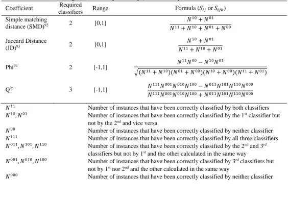
2.4. Binary diversity indices (BDIs)
BDIs quantify the dissimilarity or independency of classifications of base classifiers when they are combined in triads. This is later used to determine whether combinations of dissimilar or independent classifiers also have a corresponding high performance during voting. In the present study, the correct classification of an instance by a classifier was assigned a “1” score, whereas misclassification was assigned a “0” score. Using this binary assessment for all 10 classifiers, four well-known BDIs (Table 3) were computed. The first three BDIs are estimated by combining the classification results of two classifiers. Thus, to express dissimilarity with simple matching distance (SMD), Jaccard distance (JD) and independency (Phi) in triads, an average of the paired combinations was calculated. The last index (Q), being also a measure of independency (positive or negative) between classifiers, is estimated by using three classifiers as described in Kuncheva et al.76.
Table 3. Definition and ranges of four binary similarity (or dissimilarity) indices Coefficient Required
classifiers Range Formula (𝑆𝑖𝑗 or 𝑆𝑖𝑗𝑘) Simple matching distance (SMD)92 2 [0,1] 𝑁10+ 𝑁01 𝑁11+ 𝑁10+ 𝑁01+ 𝑁00 Jaccard Distance (JD)93 2 [0,1] 𝑁10+ 𝑁01 𝑁11+ 𝑁10+ 𝑁01 Phi94 2 [-1,1] 𝑁 11𝑁00− 𝑁10𝑁01 √(𝑁11+ 𝑁10)(𝑁01+ 𝑁00)(𝑁10+ 𝑁00)(𝑁11+ 𝑁01) Q95 3 [-1,1] 𝑁111𝑁001𝑁010𝑁100− 𝑁011𝑁101𝑁110𝑁000 𝑁111𝑁001𝑁010𝑁100+ 𝑁011𝑁101𝑁110𝑁000
𝑁11 Number of instances that have been correctly classified by both classifiers
𝑁10, 𝑁01 Number of instances that have been correctly classified by the 1st classifier but not by the 2nd and vice versa
𝑁00 Number of instances that have been correctly classified by neither classifier
𝑁111 Number of instances that have been correctly classified by all three classifiers
𝑁011, 𝑁101, 𝑁110 Number of instances that have been correctly classified by the 2nd and 3rd classifiers but not by 1st and the other calculated in the same way
𝑁001, 𝑁010, 𝑁100 Number of instances that have been correctly classified by 3rd classifiers but not by 1st nor 2nd and the other calculated in the same way
2.5. Dissimilarity-Performance index (DP)
Apart from the classifier dissimilarity within triads (quantified by the traditionally used BDIs), the individual performance of each classifier was also considered in the present study aiming to provide further information on the best set of classifiers to be combined for improved classification.96 This joint approach for the identification of the best performing classifier triad was achieved in the present study by developing an integrated Dissimilarity-Performance (DP) index. The proposed formula for this DP index is the following: 𝐷𝑃 = (1 − 𝑎) ∙∑ 𝐽𝑖,𝑗 𝑛 𝑖<𝑗 3 + 𝑎 ∙ ∑𝑛𝑖=1𝑝𝑖 3 𝑖, 𝑗 = 1,2,3 (1)
where 𝐽𝑖,𝑗 the JD index calculated from the binary classification results of the i-th and j-th
classifiers, 𝑝𝑖 is the ratio of the correctly classified samples by the i-th classifier to the
total number of instances and 𝑎 is a parameter between 0 and 1 (0 ≤ 𝑎≤ 1). The first addend represents the average of the JD for all classifier pairs, while the second is the average of the single performances of each classifier used in voting. Parameter 𝑎
expresses the different contribution of the aforementioned criteria, i.e. dissimilarity and performance of the combined classifiers. Therefore, if 𝑎 is equal to 0 the characteristic of dissimilarity among classifiers prevails in the DP index, expressing the case that better voting performance is achieved by combining classifiers showing large discrepancies among their individual predictions. On the other hand, if 𝑎 is equal to 1 only the individual performance of the base classifiers is counting in the DP index, meaning that the voting performance of the various classifier combinations is proportional solely to their individual performance. Finally, if 𝑎 = 0.5 then the two criteria have an equal contribution to the DP index. It should be noted that the DP values are always in the range 0 to 1.
The efficiency of BDIs and DP based on the performance criterion (i.e. CCI) for the 120 different classifier triads was assessed with Spearman’s rank correlation coefficient. Moreover, the DP index was calculated for many different values of the parameter 𝑎
(from 0 to 1 with a 0.01 step) for each classifier triad across the 14 training databases in order to define the value of 𝑎 that optimizes the Spearman’s rank correlation coefficient between DP and voting performance. This procedure (a) optimizes the determining force of DP in identifying the best classifier triads, (b) determines the efficiency and consistency of DP to perform substantially different classification tasks (c) offers a prioritization of the two crucial criteria of dissimilarity and performance among classifiers participating in voting. Furthermore, we tested whether DP can identify the classifier triad with the best voting performance for 14 testing (unseen) datasets. This was performed by crosschecking whether the best triad falls within the 10% of the triads (i.e. 12 triads) with the highest DP values. DP was further tested for monotonicity (consistent increase or decrease along the CCI spectrum) as this is an important prerequisite for an index.97 Finally, the DP efficiency was examined to improve the voting EM when trained with datasets containing different number of labels of the target class.
3. Results
3.1. Results of base classifiers and voting ensemble method
The classification performance of the worst and best performing base classifier along with the corresponding performance of the voting EM across all datasets are presented in Table 4. The MLPs achieved the highest performance in most databases and can be characterized as the best base classifier in this study. On the other hand, NB was the base classifier with the lowest performance showing the lowest % CCI in twelve out of 28 databases.
Table 4. Percentage of CCI for the worst and best base classifiers cited in parenthesis along with the corresponding percentage of the Voting EM for training databases. The symbol † denotes the participation of the best base classifier in the best classifier triad of Voting EM.
Database Worst base classifier performance
Best base classifier performance Voting performance (best triad) Tr ai n in g D at ab ases
ARR 52.88 (IBk) 70.35 (JRip) 71.48 (†)
BRE 64.69 (MLP) 75.52 (J48) 77.30 (†)
GER 69.40 (K*) 75.40 (NB) 76.90 (†)
GLA 48.60 (NB) 75.23 (RF) 81.71 (†)
ION 82.62 (NB) 92.88 (RF) 94.89
IRI 94.00 (Part) 97.33 (MLP) 97.33 (†)
LAB 82.46 (IBk) 92.98 (Log) 96.67 (†)
PAG 90.85 (NB) 97.01 (Part) 97.50 (†) SEG 81.07 (NB) 96.80 (MLP) 98.13 (†) VEH 44.80 (NB) 81.68 (MLP) 83.23 (†) VOT 90.11 (NB) 96.32 (J48) 97.01 (†) WAV 73.48 (K*) 86.68(SMO) 86.74 (†) BER 51.59 (NB) 81.70 (MLP) 86.73 (†)
ECO 44.15 (SMO) 63.30 (IBk) 69.15
Te st in g D at ab ases BAN 84.26 (NB) 99.93 (MLP) 100.00 (†) BLO 71.00 (NB) 85.00 (RF) 88.00 (†) CAR 85.53 (NB) 99.48 (MLP) 99.60 (†) CHR 91.75 (K*) 99.75 (RF) 100.00 (†) DER 86.89 (JRip) 97.27 (NB) 98.09 (†) FER 83.00 (IBk) 90.00 (MLP) 92.00 (†) FOR 76.31 (K*) 86.46 (SMO) 87.35 HEP 74.84 (JRip) 85.16 (RF) 87.71 LUN 37.50 (IBk) 62.50 (NB) 69.17 (†) SEE 90.48 (JRip) 95.24 (MLP) 97.14 (†) SEI 86.73 (NB) 93.42 (SMO) 93.42 (†)
TEA 40.40 (JRip) 66.23 (IBk) 66.25 (†)
WIN 44.24 (NB) 70.17 (RF) 68.58 (†)
ABD 79.46 (IBk) 86.24 (JRip) 86.81 (†)
The best combination triad of the 10 aforementioned base classifiers that trained the voting EM has shown higher classification performance (2% on average) compared to the performance of the best individual classifier for most of the databases (25 out of 28)
(Table 4). Moreover, in 4 datasets (GLA, BER, ECO and LUN) voting achieved an increase in classification performance (based in % CCI) exceeding 5%. As for the IRI and SEI databases, the voting performance was found equal to the performance achieved by the best base classifier (MLP and SMO respectively) and finally for the WIN database the voting performance was worse compared with the performance of the RF base classifier. The latter was possibly due to the relatively worse performance of all base classifiers except RF (average performance of the all other classifiers is equal to 56.44% while the second best classifier lags in performance more than 5% from RF). The best voting triad for all datasets did not always contain the best base classifier. In fact, in ION, ECO, FOR and HEP datasets the best triad contained, instead of the best base classifier, another base classifier which also achieved high performance (has in average only 1% lower performance than the best base classifier). However this classifier is much more diverse when compared with the two other members of the classifier triad (JD index increases at least 3% with this classifier instead of the best base classifier).
3.2.Results of existing BDIs
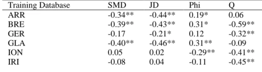
The correlations between the BDIs and the corresponding voting performance (in terms of CCI) of the classifier combinations across training datasets are presented in Table 5. JD can be characterized as the best among BDIs, showing statistically significant correlation (p<0.01) for most datasets (11 out of 14) compared to other indices. Other BDIs such as SMD were more weakly but significantly correlated (p<0.01) for 10 of the datasets, whereas Q was significantly correlated (p<0.01) with CCI only in 8 datasets. The negative correlation between SMD or JD and the voting performance shows that when combining classifiers solely based on their highly dissimilar results (i.e. without taking into account the performance criterion), the subsequent voting performance is reduced. Regarding the sign of the correlation between Q index and CCI, it was found negative in most datasets; in 3 of them (i.e. PAG, VEH and WAV) it was positive with significant correlation, showing that Q cannot consistently follow the increase of the voting performance. As a result, in some databases the combinations leading to high voting performance correspond to small Q values (negative sign of correlation) while in others to relative large (positive sign). Finally, Phi index was not correlated with voting performance for most of the classifications tasks, therefore it is considered as the least efficient BDI in this study.
Table 5. Spearman rank correlation coefficients of the performance (based on CCI%) of the voting algorithm and the BDIs.
Training Database SMD JD Phi Q
ARR -0.34** -0.44** 0.19* 0.06 BRE -0.39** -0.43** 0.31* -0.59** GER -0.17 -0.21* 0.12 -0.32** GLA -0.40** -0.46** 0.31** -0.09 ION 0.05 0.02 -0.29** -0.41** IRI -0.08 0.04 -0.11 -0.45**
LAB -0.34** -0.40** -0.11 -0.07 PAG -0.70** -0.71** 0.66** 0.18* SEG -0.72** -0.72** 0.34 -0.18 VEH -0.24** -0.38** 0.01 0.34** VOT -0.60** -0.60** 0.35** -0.37** WAV -0.61** -0.62** 0.56** 0.52** BER -0.53** -0.62** 0.00 -0.39** ECO -0.21* -0.41** 0.16 -0.15
* Significant correlation at the 0.05 level (2-tailed) ** Significant correlation at the 0.01 level (2-tailed)
3.3.Optimizing the DP index
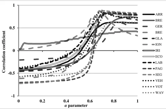
DP index incorporates two basic criteria (i.e. individual performance and the dissimilarity of base classifiers) by weighting them with parameter α (section 2.5). Since JD was the best performing BDI (showing the best correlation with voting performance across databases), it was selected to represent the dissimilarity among classifier results in DP index. In order to select the optimal value of parameter a, DP was computed along an α range from 0 to 1 with 0.01 step for all datasets. Subsequently, the correlation coefficient between DP and voting performance was computed along the parameter α range for all datasets (Fig. 2). The graph shows that for small parameter α values (i.e. the criterion of dissimilarity among classifiers results prevails in DP), the correlation coefficient starts with high negative values and approaches zero as the value of a increases (the criterion of individual performance of base classifiers getting into DP). Thereafter, the correlation coefficient changes sign and increases gradually reaching a maximum value when a is within a relative small interval (between 0.7 and 0.8 for all datasets). Above this point the correlation decreases as a approaches 1 (i.e. only individual classifier performance remains in DP). The aforementioned behavior was observed across all training datasets, except of IRI in which the correlation increases constantly when a parameter increases. This inconsistency can be explained by the fact that in this database the base classifiers had very similar performances (CCI equal to 94% and 97.33% for the worst and best classifier) (Table 4) and also by the negligible dissimilarity among the classifier results (mean JD of the 10 classifiers equal to 0.03).
Fig. 2. Change of correlation coefficient between voting performance and DP index for different values of parameter α for each training dataset.
The optimal values of parameter a (maximizing the correlation between DP and voting performance for each dataset) had relatively small variation (n=14, variance=0.004, coefficient of variation=8%) showing that the optimal value of parameter a does not considerably vary among datasets. Thus, the mean of optimal values of a estimated from all datasets was used as the most appropriate measure to determine the a value within DP index (a=0.77). The DP index was thus computed by fixing the value of parameter a at 0.77.
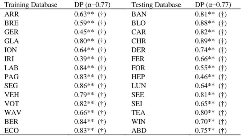
3.4.Efficiency of DP index
The correlation between DP and voting performance (in terms of CCI) for the 120 different classifier triads for all datasets is presented in Table 6. DP correlated (p<0.01) with voting performance for both training and testing datasets and the correlation coefficients were considerably high (R>0.70) in most databases. In three datasets (i.e. IRI, GER and HEP) the correlation was rather weak but still statistically significant (p<0.01). Considering that voting performance can be expressed by % CCI, the most efficient among the considered indices is DP showing consistently positive and higher correlations for all datasets. Moreover, the 12 triads (10% of the total) with the highest DP values for each testing dataset were those having the corresponding higher
-1 -0.5 0 0.5 1 0 0.2 0.4 0.6 0.8 1 Co rr ela tio n co ef ficient α parameter ARR BRE GER BRE GLA ION IRI ECO LAB PAG SEG VEH VOT WAV
performance during voting EM. The optimal triad (i.e. the one with the best voting performance) was found amongst the selected triads across testing (also for training) datasets (tick symbol in Table 6) and thus DP can be considered effective in identifying the best classifier combination.
Table 6. Spearman rank correlation coefficient of the performance (based on CCI%) of the voting algorithm and the proposed DP index trained on the 120 classifier combination triads for all datasets. The symbol † denotes the identification of the best classifier triad from the DP index.
Training Database DP (α=0.77) Testing Database DP (α=0.77)
ARR 0.63** (†) BAN 0.81** (†) BRE 0.59** (†) BLO 0.88** (†) GER 0.45** (†) CAR 0.82** (†) GLA 0.80** (†) CHR 0.89** (†) ION 0.64** (†) DER 0.74** (†) IRI 0.39** (†) FER 0.66** (†) LAB 0.84** (†) FOR 0.55** (†) PAG 0.83** (†) HEP 0.46** (†) SEG 0.86** (†) LUN 0.64** (†) VEH 0.79** (†) SEE 0.81** (†) VOT 0.82** (†) SEI 0.65** (†) WAV 0.66** (†) TEA 0.80** (†) BER 0.84** (†) WIN 0.70** (†) ECO 0.83** (†) ABD 0.75** (†)
* Significant correlation at the 0.05 level (2-tailed) ** Significant correlation at the 0.01 level (2-tailed)
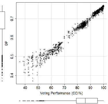
The monotonic behavior of DP was checked by plotting its variability (120 classifier triads implemented in 14 datasets=120*14=1680 points) in relation to the voting performance in terms of CCI (Fig. 3) for comparative reasons. DP has shown consistent increase along the voting CCI spectrum and thus its behavior is monotonic. The few points in which the estimated DP index was rather high (4-5 points at the left side) represent classifier triads in which one poorly performing classifier participates. In those few cases, the voting performance was greatly affected by the contribution of a poor classifier (i.e. NB for WIN dataset or IBk for LUN dataset) but DP could not incorporate such effects. However, the estimated correlation coefficient between DP and voting performance was extremely high for all points (n=1680, Spearman R=0.99, p<0.01) indicating the monotonic increase of DP across the corresponding voting performance increase expressed by % CCI. More specifically, the triads having high DP values (being of high importance because they can demonstrate the optimal classifier combinations) are those that finally achieved the best voting performances (points located on the top right of the graph).
Fig. 3. Monotonic behavior of DP along voting performance in terms of CCI% gradient for all classifier triads across training datasets (120 classifier combinations * 14 datasets = 1680 points)
The percentage of improvement in voting performance when trained with the DP proposed triad against the best base classifier across different number of labels of the target class is presented in Fig 4. This improvement in performance is approximately 1-2% for databases with 2, 3, 4 and more than 6 labels and relatively higher (around 4%) for databases with 5 or 6 labels. Thus, DP offers significant performance improvement regardless of the number of labels of the target class of the trained dataset.
Fig. 4. Percentage of improvement achieved by voting EM compared to the best base classifier in accordance with the number of labels of the target class of each dataset.
4. Discussion
In the present study, 10 base classifiers corresponding to various ML categories, were trained using 28 substantially different datasets from diverse scientific fields (e.g. Medicine, Ecology, Botany, Physics, Sociology, Economy, Web, and Engineering) in order to access their individual classifying efficiency. MLP was the best performing base classifier in contrast to NB which showed the poorest performance in agreement with previous applications.98-100 Subsequently, all possible classifier triads resulting from combinations of the 28 base classifiers were used to train the easiest and most widely applicable EM i.e. voting classifier. The best triad has shown improved performance across most datasets (except for IRI, SEI and WIN databases in which the voting performance was either equal or slightly worse compared with the best base classifier) in agreement with the general principle that ensembles of classifiers are often substantially more accurate than their individual base classifiers.20,27,29,40,101 For 4 datasets the % increase of CCI was over 5%, considered as a remarkable improvement in classification performance.12
Each base classifier employs a different learning strategy to provide its own classification results which are fed into the voting algorithm for the final classification. When the individual results are similar then the outcome will be based more or less on the same information (errors and corrects), without offering any additive value in voting, increasing however the system complexity.25,26,35,102 On the other hand, EMs consisting of classifiers offering different results have the potential to achieve significantly better performance compared to those of individual base classifiers.15,19,35,39,103 This finding was confirmed in the present study, with SMC and JD dissimilarity measures showing statistically significant correlations with voting performance for most of the training datasets. More specifically JD scored higher (absolute) values of correlation than the comparable SMC index rather because it emphasizes on differences between classifier results.104 However, the two measures of independency (i.e. Q and Phi) that were supposed to improve voting accuracy,17,76,105 showed low correlation with voting performance also in agreement with some previous studies.35,36,38
Although dissimilarity among individual classifiers combined to develop EMs may be the key towards improving classification efficiency,88 dissimilar but powerless classifiers are unlikely to bring any benefits in EMs performance.35,106 The latter was confirmed in the present study by the negative sign of correlation indicating that classifier triads with highly differentiated results (as expressed by JD or SMC) often contain at least one poor classifier which significantly affects the voting performance. In addition, the relative high correlation between the voting performance and the individual performances (when a=1 in DP) of base classifiers denoted for the training datasets, indicates that the individual performance is a rather crucial characteristic in optimizing EMs as previously
suggested.18,107,108 Thus, both accurate and diverse classifiers are needed in order to construct combinations that optimize the voting performance.
These two crucial characteristics, dissimilarity and individual performance of combined classifiers, have been integrated in the present study in a new index selecting the optimum classifier combinations to train the voting algorithm. The DP index integrates dissimilarity using the JD measure, which is generally considered as an efficient and stable indicator.109 In the present study JD was the most sensitive among the BDIs on following the voting performance variability. This is in agreement with Kuncheva and Hadjitodorov110 who employed JD in cluster ensembles. In addition, DP index integrates the performance characteristic using the individual performance of the classifiers, as it is widely accepted and also proved in the present study that optimal combinations should include classifiers with high individual performances.24,47
The dissimilarity and the individual performance of classifier combinations were weighted in DP using parameter α. The optimal value of this parameter (maximizing the correlation between DP and voting performance) did not vary significantly among the 14 substantially different training datasets suggesting that the DP performance is consistent and robust across different classification tasks. Subsequently, the determined DP outperformed all BDIs by showing statistically significant correlation with the voting performance across all training datasets. The same correlation was also found statistically significant for all testing datasets, the values of the correlation coefficient being relatively high (R>0.7 in most cases). These findings show that DP index is both efficient and consistent, being highly correlated with voting performance. Moreover, the optimization of DP offered a prioritization between the two characteristics of the classifier combinations with the dissimilarity weighting almost three times less than the individual performance (a=0.77). This prioritization makes DP efficient in determining the best performing classifier triad during voting for all datasets, even for those (ION, ECO, FOR and HEP) where the best triad did not contain the base classifier with the best individual performance. In these datasets, the best triads contain classifiers with relatively lower performance compared to the best, however with sufficiently dissimilar results which maximize DP value. This finding shows that DP performs better than methods proposing triads including by default the best performing base classifier.41 Furthermore, DP showed a monotonic increase across the voting performance spectrum (R>0.95) regardless of the testing dataset suggesting that it closely matches the voting performance. This matching was achieved even for datasets where voting EM performed lower than the best base classifier (i.e. WIN), in which although DP managed to determine the best triad. Finally, DP offered significant improvement (as least 1%) in the ensemble performance regardless of the number of labels of the target class.
In this paper, a new index named DP was proposed in order to rank the classifier combinations according to their performance during voting training. Based on the simulation results, comparisons and discussion we have the following conclusions: (1) Both individual performance and dissimilarity in classification outcomes when
classifiers participate in voting are crucial criteria affecting the voting performance.
(2) DP which optimally incorporates the above characteristics (i.e. individual performance and dissimilarity) achieved an efficient ranking of classifier combinations according to their voting performance.
DP is a useful tool for the individual users aiming to identify the optimal classifier combinations to use in voting EM, in order to easily achieve improved classification performance using their own familiar and tested ML algorithms. Apart from the easiness of application, DP has a number of additional advantages i.e. simplicity (it uses only three combined classifiers), efficiency (it successfully selects the classifiers to participate in the voting algorithm), flexibility (any base classifier can be included in the DP computation) and consistency (robust performance across substantially different datasets). On the other hand, DP cannot be compared with EM schemes that perform thorough search towards inducing all possible kinds of classification errors which however need qualified designers to apply them to new tasks. Finally, in datasets where the training of voting EM results in lower performance compared to the individual base classifiers, DP still defines the optimal classifier triad which however is not improving the performance of the requested classification issue.
References
1. J. G. Carbonell, R. S. Michalski and T. M. Mitchell, An overview of machine learning, in
Machine Learning, eds. R. S. Michalski, J. G. Carbonell and T. M. Mitchell (Springer, Berlin/Heidelberg, 1983), pp. 3-23.
2. S. B. Kotsiantis, I. D. Zaharakis and P. E. Pintelas, Machine learning: a review of
classification and combining techniques, Artificial Intelligence Review26(3) (2006) 159-190.
3. C. Apte, R. Sasisekharan, V. Seshadri and S. M. Weiss, Case studies in high-dimensional
classification, Applied Intelligence4(3) (1994) 269-281.
4. G. Huang, G. B. Huang, S. Song and K. You, Trends in extreme learning machines: a review,
Neural Networks61 (2015) 32-48.
5. M. Kuramochi and G. Karypis, Gene classification using expression profiles: a feasibility
study, International Journal of Artificial Intelligence Tools14(4) (2005) 641-660.
6. Y. Shi, Y. Gao, R. Wang, Y. Zhang and D. Wang, Transductive cost-sensitive lung cancer
image classification, Applied Intelligence38(1) (2013) 16-28.
7. I. Koprinska, J. Poon, J. Clark and J. Chan, Learning to classify e-mail, Information Sciences
177(10) (2007) 2167-2187.
8. M. Brescia, S. Cavuoti, M. Paolillo, G. Longo and T. Puzia, The detection of globular
clusters in galaxies as a data mining problem, Monthly Notices of the Royal Astronomical
Society421(2) (2012) 1155-1165.
9. G. Tsekouras, H. Sarimveis, C. Raptis and G. Bafas, A fuzzy logic approach for the
classification of product qualitative characteristics, Computers & Chemical Engineering
26(3) (2002) 429-438.
10. K. Topouzelis and D. Kitsiou, Detection and classification of mesoscale atmospheric
phenomena above sea in SAR imagery, Remote sensing of environment160 (2015) 263-272.
11. D. Lu and Q. Weng, A survey of image classification methods and techniques for improving
classification performance, International Journal of Remote Sensing28(5) (2007) 823-870.
12. M. Pal and P. M. Mather, An assessment of the effectiveness of decision tree methods for
land cover classification, Remote Sensing of Environment86 (4) (2003) 554-565.
13. N. Japkowicz, Supervised versus unsupervised binary-learning by feedforward neural
networks, Machine Learning42(1-2) (2001) 97-122.
14. S. B. Kotsiantis, Supervised learning: A review of classification techniques, Informatica31
(2007) 249-268.
15. L. I. Kuncheva, Combining pattern classifiers: methods and algorithms, 2nd edn. (Wiley,
New Jersey, 2014).
16. B. B. Chaudhuri and U. Bhattacharya, Efficient training and improved performance of
multilayer perceptron in pattern classification, Neurocomputing34(1-4) (2000) 11-27.
17. P. Baldi, S. Brunak, Y. Chauvin, C. A. F. Andersen and H. Nielsen, Assessing the accuracy
of prediction algorithms for classification: An overview, Bioinformatics 16(5) (2000)
412-424.
18. D. W. Opitz and R. Maclin, Popular ensemble methods: an empirical study, Journal of
19. Z. Liu, Q. Dai and N. Liu, Ensemble selection by GRASP, Applied Intelligence41(1) (2014) 128-144.
20. Z. H. Zhou, Ensemble methods – Foundations and algorithms, (Chapman & Hall/CRC,
Florida, 2012).
21. C. N. Anagnostopoulos, T. Iliou and I. Giannoukos, Features and classifiers for emotion
recognition from speech: a survey from 2000 to 2011, Artificial Intelligence Review42(2)
(2012) 1-23.
22. M. Wozniak, M. Grana and E. Conchado, A survey of multiple classifier systems as hybrid
systems, Information Fusion16 (2014) 3-17.
23. E. Bauer and R. Kohavi, An empirical comparison of voting classification algorithms:
bagging, boosting, and variants. Machine Learning36(1-2) (1999) 105-139.
24. T. G. Dietterich, An experimental comparison of three methods for constructing ensembles of
decision trees: bagging, boosting, and randomization, Machine Learning 40(2) (2000)
139-157.
25. A. C. Tan and D. Gilbert, Ensemble machine learning on gene expression data for cancer
classification, Applied Bioinformatics2 (2003) S75-S83.
26. A. Ulas, M. Semerci, O. T. Yildiz and E. Alpaydin, Incremental construction of classifier and
discriminant ensembles, Information Sciences179(9) (2009) 1298-1318.
27. A. Onan, S. Korukoglu and H. Bulut, A multiobjective weighted voting ensemble classifier
based on differential evolution algorithm for text sentiment classification, Expert Systems
with Applications 62 (2016) 1-16.
28. G. Tsoumakas, I. Katakis and I. Vlahavas, Effective Voting of Heterogeneous Classifiers, in:
Machine Learning: ECML 2004, eds. J. F. Boulicaut, F. Esposito, F. Giannotti, D. Pedreschi (Springer, Berlin/Heidelberg, 2004) pp. 465-476.
29. S. Saha and A. Ekbal, Combining multiple classifiers using vote based classifier ensemble
technique for named entity recognition, Data & Knowledge Engineering85 (2013) 15-39.
30. N. Dimililer, E. Varoglu and H. Altincay, Classifier subset selection for biomedical named
entity recognition, Applied Intelligence31(2009) 267-282.
31. E. Dimitriadou, A. Weingessel and K. Hornik, Voting-Merging: An ensemble method for
clustering, in: Artificial Neural Networks-ICANN 2001, eds. G. Dorffner, H. Bischof, K.
Hornik , (Springer, Berlin/Heidelberg, 2001), pp. 217-224.
32. E. Loza Mencia, S. H. Park and J. Furnkranz, Efficient voting prediction for pairwise
multilabel classification, Neurocomputing73(7-9) (2010) 1164-1176.
33. H. Ishibuchi, T. Nakashima and T. Morisawa, Voting in fuzzy rule-based systems for pattern
classification problems, Fuzzy Sets and Systems103(2) (1999) 223-238.
34. V. G. Kaburlasos and T. Pachidis, A Lattice-Computing ensemble for reasoning based on
formal fusion of disparate data types, and an industrial dispensing application, Information
Fusion16 (2014) 68-83.
35. D. Ruta and B. Gabrys, Classifier selection for majority voting, Information Fusion 6(1)
(2005) 63-81.
36. R. E. Banfield, L. O. Hall, K. W. Bowyer and W. P. Kegelmeyer, Ensemble diversity
37. L. I. Kuncheva and C. J. Whitaker, Measures of diversity in classifier ensembles and their
relationship with the ensemble accuracy, Machine Learning51(2) (2003) 181-207.
38. A. Shipp and L. I. Kuncheva, Relationships between combination methods and measures of
diversity in combining classifiers, Information Fusion 3(2) (2002) 135-148.
39. I. Perikos and I. Hatzilygeroudis, Recognizing emotions in text using ensemble of classifiers,
Engineering Applications of Artificial Intelligence51 (2016) 191-201.
40. G. Rudolph and T. Martinez, Finding the real differences between learning algorithms,
International Journal on Artificial Intelligence Tools24(3) (2015).
41. A. Tamvakis, G. E. Tsekouras, A. Rigos, C. Kalloniatis, C. N. Anagnostopoulos and G.
Anastassopoulos, A methodology to carry out voting classification tasks using a particle
swarm optimization-based neuro-fuzzy competitive learning network, Evolving Systems8(1)
(2017) 49-69.
42. M. Amini, J. Rezaeenour and E. Hadavandi, A neural network ensemble classifier for
effective intrusion detection using fuzzy clustering and radial basis function networks,
International Journal on Artificial Intelligence Tools25(2) (2016).
43. Z. H. Zhou, Clusterer ensemble, Knowledge-Based Systems19(1) (2006) 77-83.
44. J. S. Chou, C. F. Tsai, A. D. Pham and Y. H. Lu, Machine learning in concrete strength
simulations: Multi-nation data analytics, Construction and Building Materials73 (2014)
771-780.
45. F. Roli and G. Giacinto, Design of multiple classifier systems, in: Hybrid Methods in Pattern
Recognition, eds. H. Bunke and A. Kandel, (Worldwide Scientific Publishing, Singapore, 2002) pp 199-226.
46. N. Garcia-Pedrajas, J. Maudes-Raedo, C. Garcia-Osorio and J. J. Rodriguez-Diez, Supervised
subspace projections for constructing ensembles of classifiers, Information Sciences 193
(2012) 1-21.
47. G. Giacinto and F. Roli, An approach to the automatic design of multiple classifier systems,
Pattern Recognition Letters22(1) (2001) 25-33.
48. W. Opitz and J. W. Shavlik, Actively searching for an effective neural network ensemble,
Connection Science8(3-4) (1996) 337-353.
49. M. Hall, E. Frank, G. Holmes, B. Pfahringer, P. Reutemann and I. H. Witten, The WEKA
data mining software: an Update, SIGKDD Explorations11(1) (2009) 10-18.
50. F. Burkhardt, A. Paeschke, M. Rolfes, W. Sendlmeier and B. Weiss, A database of German
emotional speech. in: Proc. 9th Int. Conf. on Spoken Language Processing
(INTERSPEECH-ICSLP, Lissabon, 2005) pp. 1517-1520.
51. P. Boersma and D. Weenink, Praat: doing phonetics by computer (version 4.6.09) (2005),
http://www.praat.org.
52. N. Anagnostopoulos and T. Iliou, Towards emotion recognition from speech: definition,
problems and the materials of research, in: Semantics in Adaptive and Personalized Services,
eds. M. Wallace, I. Anagnostopoulos, P. Mylonas and M. Bielikova, (Springer, Berlin/Heidelberg, 2010), pp. 127-143.
53. S. Spatharis, G. Tsirtsis, D. B. Danielidis, D. C. Thang and D. Mouillot, Effects of pulsed nutrient inputs on phytoplankton assemblage structure and blooms in an enclosed coastal
area, Estuarine, Coastal and Shelf Science73(3-4) (2007) 807-815.
54. N. Simboura, P. Panayotidis and E. Papathanassiou, A synthesis of the biological quality
elements for the implementation of the European Water Framework Directive in the
Mediterranean ecoregion: The case of Saronikos Gulf, Ecological Indicators5(3) (2005)
253-266.
55. A. Tamvakis, C. N. Anagnostopoulos, G. Tsekouras and G. Anastassopoulos, Optimizing
voting classification using cluster analysis on medical diagnosis data, in: Proc. 16th Int. Conf.
on Engineering Applications of Neural Networks (EANN'15, Rhodes, Greece, 2015) pp. 1-7.
56. A. Deshmukh, A. S. Patil and B. V. Pawar, Comparison of classification algorithms using
WEKA on various datasets, International Journal of Computer Science and Information
Technology4(2) (2011) 85-90.
57. R. C. Holte, Very simple classification rules perform well on most commonly used datasets,
Machine Learning11(1) (1993) 63-90.
58. M. Varna and R. B. Bolda, More generality in efficient multiple Kernal learning, in: Proc.
26th Annual Int. Conf. on Machine Learning (ICML, Montreal, Quebec, Canada) (2009) pp. 1062-1072.
59. S. W. Lin and S. C. Chen, PSOLDA: A particle swarm optimization approach for enhancing
classification accuracy rate of linear discriminant analysis, Applied Soft Computing9 (2009)
1008-1015.
60. S. Ozsoy, G. Gumus and S. Khalilov, C4.5 versus other decision trees: A review, Computer
Engineering and Applications 4 (2015) 173-181.
61. I. Sangaiah, A. V. A. Kumar, A. Balamurugan, An empirical study on different ranking
methods for effective data classification, Journal of Modern Applied Statistical Methods
14(2) (2015) 35-52.
62. A. Iranzad, A. Masoudnia, F. Cheraghchi, A. Nowzari-Dalini, R. Ebrahimpour, Improving
combination methods of neural classifiers using NCL, International Journal of Computer
Information Systems and Industrial Management Applications4 (2012) 679-686
63. D. Koller and M. Sahami, Toward optimal feature selection, in: Proc. 13th Int. Conf. on
Machine Learning (Bari, Italy, 1996) pp. 284-292.
64. J. Wang and G. Karypis, HARMONY: Efficiently mining the best rules for classification, in:
Proc. 5th Int. Conf. on Data Mining (SIAM, California, 2005) pp. 205-216.
65. N. I. Nife, Performance analaysis of various data mining techniques on banknote
authentication, International Journal of Engineering Science Invention5(2) (2016) 62-71.
66. Y. Asim, A. R. Shahid, A. K. Malik, B. Raza, Significance of machine learning algorithms in
professional blogger's classification, Computers and Electrical Engineering (In Press 2017)
1-33.
67. A. Selekin and J. Stankovic, Detection of chronic kidney disease and selecting important
predictive attributes, in: IEEE Int. Conf. on Healthcare Informatics (ICHI, Chicago, 2016)
68. D. Gil, J. L. Girela, J. De Juan, M. J. Gomez-Torres, and M. Johnsson, Predicting seminal
quality with artificial intelligence methods, Expert Systems with Applications39(16) (2012)
12564-12573.
69. B. Johnson, R. Tateishi and Z. Xie, Using geographically-weighted variables for image
classification, Remote Sensing Letters3(6) (2012) 491-499.
70. V. Singh, L. Mukherjee, J. Peng and J. Xu, Ensemble clustering using semidefinite
programming with applications, Machine Learning 79 (2010) 177-200.
71. M. Charytanowicz, J. Niewczas, P. Kulczycki, P. A. Kowalski, S. Lukasik and S. Zak,
Complete gradient clustering algorithm for features analysis of x-ray images, in: Information
Technologies in Biomedicine, eds. E. Pietka, J. Kawa (Springer, Berlin/Heidelberg, 2010) pp. 15-24.
72. D. Bertsimas and J. Dunn, Optimal classification trees, Machine Learning106 (2017)
1039-1082.
73. P. Cortez, A. Cerdeira, F. Almeida, T. Matos and J. Reis, Modeling wine preferences by data
mining from physicochemical properties, Decision Support Systems47 (2009) 547-533.
74. T. Iliou, C. N. Anagnostopoulos, I. Stephanakis and G. Anastassopoulos, Combined
classification of risk factors for appendicitis prediction in childhood, in: Engineering
Applications of Neural Networks, eds. L. Iliadis, H. Papadopoulos and C. Jayne, (Springer, Berlin/Heidelberg, 2013), pp. 203-211.
75. S. Dzeroski and B. Zenko, Is combining classifiers with stacking better than selecting the best
one?, Machine Learning54(3) (2004) 255-273.
76. L. I. Kuncheva, C. J. Whitaker, C. A. Shipp and R. P. W. Duin, Is independence good for
combining classifiers?, in: Proc.15th Int. Conf. on Pattern Recognition, (Barcelona, 2000),
pp. 168-171.
77. G. Zhou, D. Shen, J. Zhang, J. Su and S. Tan, Recognition of protein/gene names from text
using an ensemble of classifiers, BMC Bioinformatics6 (2005) S7.
78. W. W. Cohen, Fast effective rule induction, in: Proc.12th Int. Conf. on Machine Learning,
(Morgan Kaufmann, San Francisco, 1995), pp.115-123.
79. H. Witten and E. Frank, Generating accurate rule sets without global optimization, in: Proc.
15th Int. Conf. on Machine Learning, (Morgan Kaufmann, San Francisco, 1998) pp. 144-151.
80. J. R. Quinlan, C4.5: Programs for Machine Learning, (Morgan Kaufmann, San Francisco,
1993).
81. L. Breiman, Random Forests, Machine Learning45(1) (2001) 5-32.
82. W. Aha, D. Kibler and M. K. Albert, Instance-based learning algorithms, Machine Learning
6(1) (1991) 37-66.
83. J. G. Cleary and L. E. Trigg, K*: An instance-based learner using an entropic distance
measure, in: Proc.12th Int. Conf. on Machine Learning, (Morgan Kaufmann, San Francisco,
1995), pp. 108-114.
84. S. le Cassie and J. C. van Houwelingen, Ridge estimators in logistic regression, Applied
Statistics41 (1992) 191-201.
85. S. K. Pal and S. Mitra, Multilayer perceptron, fuzzy sets, and classification, IEEE
86. J. C. Platt, Fast training of support vector machines using sequential minimal optimization, in: Advances in Kernel Methods-Support Vector Learning, eds. B. Scholkopf, C. J. C. Burges and A. Smola, (MIT Press, Cambridge USA, 1998), pp. 185-208.
87. H. John and P. Langley, Estimating continuous distributions in Bayesian classifiers, in: Proc.
11th Conf. on Uncertainty in Artificial Intelligence, (Morgan Kaufmann, San Francisco, 1995), pp. 338-345.
88. J. Kittler, M. Hatef, R. W. D. Duin, and J. Matas, On combining classifiers, IEEE
Transactions on Pattern Analysis and Machine Intelligence 20(3) (1998) 226-239.
89. M. Stone, Cross-validation and multinomial prediction, Biometrika 6(3) (1974) 509-515.
90. I. H. Witten and E. Frank, Data Mining - Practical Machine Learning Tools and Techniques,
(Morgan Kaufmann, San Francisco, 2005).
91. T. H. Hoang, K. Lock, A. Mouton and P. L. M. Goethals, Application of classification trees
and support vector machines to model the presence of macroinvertebrates in rivers in
Vietnam, Ecological Informatics5(2) (2010) 140-146.
92. R. R. Sokal and P. H. A. Sneath, Principles of numerical taxonomy, (W. H. Freeman, San
Francisco, 1963).
93. P. Jaccard, Nouvelles recherctus sur la distribution floral, Bulletin Society Science Naturale
44 (1908) 223-270.
94. U. Yule, On the methods of measuring the association between two variables, Journal of the
Royal Statistical Society 75 (1912) 579-642.
95. G. U. Yule, On the association of attributes in statistics. Philosophy of Transactions A 194
(1900) 257-319.
96. A. J. C. Sharkey and N. E. Sharkey, Combining diverse neural nets, The Knowledge
Engineering Review12(3) (1997) 231-247.
97. S. Spatharis and G. Tsirtsis, Ecological quality scales based on phytoplankton for the
implementation of Water Framework Directive in the Eastern Mediterranean, Ecological
Indicators10(4) (2010) 840-847.
98. J. Boccard, A. Kalousis, M. Hilario, P. Lanteri, M. Hanafi, G. Mazerolles, J. L. Wolfender, P.
A. Carrupt and S. Rudaz, Standard machine learning algorithms applied to UPLC-TOF/MS metabolic fingerprinting for the discovery of wound biomarkers in Arabidopsis thaliana,
Chemometrics and Intelligent Laboratory Systems104(1) (2010) 20-27.
99. I. De Falco, A. Della Cioppa and E. Tarantino, Automatic classification of handsegmented
image parts with differential evolution, in: Applications of Evolutionary Computing, eds. F.
Rothlauf, J. Branke, S. Cagnoni, E. Costa, C. Cotta, R. Drechsler, E. Lutton, P. Machado, J. Moore, J. Romero, G. Smith, G. Squillero and H. Takagi, (Springer, Berlin Heidelberg, 2006) pp. 403-414.
100. M. Roshandel, A. Munjal, P. Moghadam, S. Tajik and H. Ketabdar, Multi-sensor finger ring
for authentication based on 3D signatures, in: 16th Int. Conf. Human-Computer Interaction,
Advanced Interaction Modalities and Techniques, ed. M. Kurosu, (Springer, 2014), pp. 131-138.
101. T. G. Dietterich, Machine learning research: Four current directions, AI Magazine 18(4)