R. Pasupathy, S.-H. Kim, A. Tolk, R. Hill, and M. E. Kuhl, eds.
A SIMULATION-BASED APPROACH TO ANALYZE THE INFORMATION DIFFUSION IN MICROBLOGGING ONLINE SOCIAL NETWORK
Maira A de C Gatti Ana Paula Appel Cicero Nogueira dos Santos
Claudio Santos Pinhanez Paulo Rodrigo Cavalin
Samuel Barbosa Neto
IBM Research-Brazil
Av. Tut´oia 1157, Para´ıso, S˜ao Paulo (SP), BRAZIL
ABSTRACT
In this paper we propose a stochastic multi-agent based approach to analyze the information diffusion in Microblogging Online Social Networks (OSNs). OSNs, like Twitter and Facebook, became extremely popular and are being used to target marketing campaigns. Key known issues on this targeting is to be able to predict human behavior like posting a message with regard to some topics, and to analyze the emergent behavior of such actions. We explore Barack Obama’s Twitter network as an egocentric network to present our simulation-based approach and predictive behavior modeling. Through experimental analysis, we evaluated the impact of inactivating both Obama and the most engaged users, aiming at understanding the influence of those users that are the most likely to disseminate information over the network.
1 INTRODUCTION
Online social networks (OSNs) have become very popular in the last years, not only for users but also for researchers. In this context, Twitter is just a few years old and has attracted much attention already (Kwak, Lee, Park, and Moon 2010). Through OSNs, users connect with each other, share and find content, and disseminate information.
Nowadays, OSNs are the most used way of information diffusion, a process for widely spreading a new idea or action through communication channels (Rogers and Rogers 2003). Information diffusion has been widely studied by sociologists, marketers, and epidemiologists (Kempe, Kleinberg, and Tardos 2003, Leskovec, Adamic, and Huberman 2006, Strang and Soule 1998). Large OSN are useful for studying information diffusion as topic propagation in blogspace (Gruhl et al. 2004), linking patterns in blog graph (Leskovec and Horvitz 2008), favorite photo marking in a social photo sharing service (Cha, Mislove, and Gummadi 2009), among others. In this case, understanding how users behave when they connect to these sites is important for a number of reasons. In viral marketing, for instance, one might want to exploit models of user interactions to spread their content or promotions quickly and widely. Although there are numerous models of influence spread in social networks that try to model the process of adoption of an idea or a product, it is still difficult to measure and predict how a market campaign will spread in an OSN. One style of modeling that is consistent with the sciences of complexity is agent-based simulation (ABS) (Jennings 2001). In a multi-agent system, many software agents interact among themselves and with the environment. ABS looks at agent behavior at a decentralized level, at the level of the individual agent, in order to explain the dynamic behavior of the system at the macro-level. Agents are autonomous entities: an agent is capable of acting without direct external intervention. Multi-agent systems can handle
the complexity of solutions through decomposing, modeling and organizing the interrelationships between components (Jennings 2001). Also, the locality is an intrinsic feature of an agent: the agents’ decisions are made considering the local environment and not the global one. Finally, feedback loops can be achieved in ABS, since the result of agent actions stimulates other actions and eventually re-stimulates the first actions. Simulation has been applied with success in a large number of works (Macal and North 2010). However, for the study of information diffusion in large OSNs there is still a lack of work. Most works in information diffusion models based on agents use synthetic networks for deriving the agents behavior, making the work less realistic (Janssen and Jager 2003, Delre, Jager, and Janssen 2007, Wicker and Doyle 2012). For this reason, in this work we aim at using a real online social network to simulate the user’s behavior based on what they post on OSN to analyze how the information is spread across a network. The proposed method uses a stochastic multi-agent based approach where each agent represents a user in the OSN. We consider as a case study a political campaign in microbloging Twitter, more specifically Barack Obama’s Twitter network during 2012 United States presidential race. To conduct this study, instead of using the partial OSN, we use an egocentric social network which examines only immediate neighbors and their associated interconnections.We use the simulator to evaluate the impact of removing top engaged users aiming at finding those users that have great impact on the information flow.
2 PROBLEM DESCRIPTION
We consider as the value of an egocentric follower network its ability to propagate fast and to a large number of nodes messages about the egocenter of the network. Therefore in particular, consider a sample of Barack Obama’s Twitter networks during the 2012 United States presidential race. We would like to first understand when the users will post a message about Barack Obama, then to find out which users are the most likely to disseminate information through the network about that topic. This problem can be extended to any topic and also to the polarity of the message, although we are not exploring the polarity here. Nevertheless there are two questions that we would like to answer: (i) what would happen if the seed of the network is inactive, that is, the node that represents Barack Obama? (ii) What would happen if the top most engaged users (excluding Obama) are inactive? There are two hypothesis derived from these questions that we would like to test:
Hypothesis 1 When the seed of the network is inactive, the influence around the topics spread by the seed drops considerably.
One would imagine that an egocentric network has a great value for the seed because of his/her high influence on the topics related to him/her. So if we sample data in a time frame where there are external events influencing both the seed and the seed’s network, we would expect to observe this behavior.
Hypothesis 2When the top N most engaged users that are also the seed’s direct followers are inactive, the influence spread by these users drops considerably.
Analogous, theN most engaged users that are also direct followers of the seed are expected to play a key role on influencing an egocentric social network. Here we defineengagementasthe degree to which the user reacts to his/her followees/leaders measured by the proportion between the number of messages that he/she propagates and the number of received messages. Therefore we would expect to observe a considerable dropping on the volume of messages without these users as a consequence of their influence’s decreasing.
Although these hypothesis might look like tautologies, emergent behavior is hard to predict and control, specially when we are dealing with thousand of agents whose behaviors we are predicting from historical data and finally feeding these predicted models into the simulator. Feedback loops, which briefly is the phenomena that happens when one action triggers another action which in turn trigger the former action, play a key role on possible candidates that invalidate the hypothesis on information diffusion analysis.
3 RELATED WORK
There are different types of information diffusion analysis that are related to this work: static and dynamic models. Static models approaches are mainly based on building weighted social networks as graphs and analyzing topologies and features like betweenness centrality (Delre, Jager, and Janssen 2007, Kempe, Kleinberg, and Tardos 2003, Gruhl et al. 2004). Information diffusion analysis from data can be found in (Goyal, Bonchi, and Lakshmanan 2010), although simulation technologies are not employed in that work. Regarding dynamic models, the voter model seems to be the precursor of this area (Holley and Liggett 1975). It captures the effects of only a single influence mechanism, requiring that a single random individual completely adopts the full opinion of a random neighbor. Cascade models (Saito, Nakano, and Kimura 2008) have received a lot of attention too. Some cascade models give a formal exposition of influence. For instance, the leverage of multiple influence mechanisms and relations for propagating information throughout social networks is presented in (Wicker and Doyle 2012).
On the other hand, there are approaches that propose a propagation model based on users’ preferences and personalities, and analyze the information diffusion for, for instance, market share (Janssen and Jager 2003). In addition, there are simulation models built to analyze the rumor or viral behavior as an emergent behavior (Liu and Chen 2011), but these simulation approaches are not learning the behavior of the users from real data. The simulation is created with synthetic data and a general model is analyzed which differs from our approach. At the same time there are several approaches to learn the user behavior in social networks from real data (Bonchi et al. 2011, Bachrach et al. 2012), but since the goal is not simulation, but only analysis, these behaviors models cannot be reused as an input to a simulation model. We present in this paper an approach to fill this gap.
4 DATA COLLECTION AND TEXT ANALYTICS
There exist several network sampling methods, among them we can cite node sampling, edge sampling, and snowball sampling (Lee, Kim, and Jeong 2009). A snowball sample is created by randomly selecting one seed node and performing a breadth-first search, until the number of selected nodes reaches the desired sampling ratio (Lee, Kim, and Jeong 2009). In this work we consider snowball sampling because it is more feasible, since only a fraction of nodes or edges in node or edge sampling are randomly selected and it would be difficult to do this in an OSN. Moreover, those sampling methods have a high probability of producing a network with isolated clusters (Ahn et al. 2007).
We developed an algorithm to sample an egocentric network: a network that considers a node (person) as focal point and its adjacency. We refer to this node as the seed node hereafter. This algorithm relies on a set of categories to identify the nodes according to the information we have about them. The four categories we consider are: Identified, where the only information we have from these nodes are their IDs, a unique value that identifies each user;Consulted, which are nodes for which we have already acquired metadata about them, such as the number of followers, user language and so on;Visited, comprising nodes previously marked as Consulted for which we extracted also a list of some or all followers of each; and Extracted, consisting of nodes that were previously marked asVisitedand from which a number of messages has been collected.
The sampling algorithm works as follows. First, the seed node is categorized asVisited, and all of its followers (nodes that are directly adjacent to the seed) are marked asIdentified. After that, we consult a subset of nodes randomly picked from the latter set, and mark them asConsulted. From these, we sample another subset, visit them (they are marked asVisitedconsequently), and some of its adjacent nodes are set toIdentified. Next, we select another subset of nodes from these identified nodes, set them to Consulted, and visit some randomly selected nodes, marking them as Visited as a result. This procedure is repeated until the desired maximum distanceD (from the root node) is reached. Finally, the extraction procedure is carried out. From all Visited nodes, starting with the nodes that are adjacent to the seed, we randomly
choose some of them, extract their messages within a given time window, and mark them as Extracted. We select some of their adjacent nodes, and repeat this process until the maximum distanceDis reached. Twitter’s API version 1.0 (the latest version of the API available when this sampling was conducted) presents the following limitations. The number of nodes that could be consulted was 100 nodes per request. The number of IDs that could be retrieved per request was limited to 5000. And the number of tweets that could be retrieved was 200 tweets per request. Accordingly, to extract up to 3200 tweets per user, the extraction procedure had to be processed 16 times at most. This procedure would stop when the API limit was reached, when all tweets were extracted, or when the oldest extracted tweet reached a specific date.
In order to implement the sampling algorithm, we set the maximum distance Dto 2 to the following reasons. A previous work, known as “six degree of separation” (Milgram 1967), states that with 6 steps we are usually able to reach most of the network’s nodes, starting in any node. On the other hand, it is reasonable to think that with distance 2 we are able to reach most of the network if we start at a high degree node. Since Obama has 23 millions of followers and the average number of followers in Twitter is around 100, performing a naive count without considering transitivity, we would have around 2 billion users in the second level (distance 1 from Obama). That number is higher than the number of Twitter users (1 billion). Thus, using distance 2 should be enough to analyse how information spread across this network, since it is reasonable to assume that it should be possible to reach most of Twitter‘s users with 2 steps from Obama. Of course, if we choose another seed (user) for an egocentric network or if we use other OSN, this statistics may change slightly. But this observation may remain true in most cases where high degree seeds are considered.
Then, we executed the algorithm in the following way. Since the egocentric network is centered on Barack Obama, we first marked Barack Obama‘s node asVisited and all of its followers were marked as Identified. Afterwards, we randomly picked 40k of his followers (nodes distance 1 from Obama), set them toConsulted, and from these, we randomly chose 10k to visit (they were marked asVisited then) among the ones with the language set to English. For each of these 10k nodes, we marked up to 5k of its followers asIdentified. Among them, a subset of up to 200k randomly chosen nodes, the distance of which were 2 from Obama, were set asConsulted. From these 200k, we marked up to 40k randomly selected nodes as Visited, whereas their profile language was set to English also. In the end of this process, the network that we obtained contained approximately 32 thousand nodes and the extraction process took place in the week starting on October 26th 2012. Note that the parameters used in the algorithm were defined empirically.
After that, we started extracting the tweets. Our threshold date was September 22nd and we started crawling backwards from October 26th from 2012. Therefore, we gathered twitters data from about an one-month time window. In this case, we extracted Obama‘s tweets and also the tweets from the 10k Visitednodes with distance 1 and the 40kVisited nodes with distance 2. In the end, we had approximately 5 million tweets and 24,526 nodes. Unfortunately, though, owing to the API limitations we have not been able to extract all tweets of all users (especially users that sent a high number of tweets in that period).
More details about the sampled dataset are presented in table 1. Table 1: Sampled Data and Graph
Tweets Active Users Direct Followers Edges Triangles 5.6M 24,526 3,594 160,738 83,751
4.1 Topic Classification
Before beginning the modeling approach, it is necessary to perform topic classification and, if the case, any sentiment analysis. The topic classification task consists in classifying a tweet as related to a certain topic or campaign (about politics, marketing, etc). While the sentiment analysis task has the objective to classify a tweet as a positive or negative sentence. In this paper we are not exploring the hypothesis 1 and 2 considering sentiment analysis, therefore this section only explain the topic classification that we
performed. We used a keyword based approach. First, we selected a list of keywords to represent each topic. Next, each tweet text was split into tokens using blank spaces and punctuation marks as separators. Then, the tokenized tweet is discarded or classified as belonging to one of the interesting topics, as follows:
• If the tweet contains keywords from more than one topic, it is discarded;
• If the tweet does not contain any keyword from any topic, it is classified as Other topic;
• If the tweet contains at least one keyword from a topic, it is classified as belonging to that topic.
We discarded the tweets that contained keywords from more than one topic because we did not tackle the problem of ambiguity.
The keywork list used to Obama topics includes the words: barack, barack2012, barackobama, biden, joebiden, josephbiden, mrpresident, obama, obama2012, potus. Note that we also considered hashtags (e.g. #obama,#gobama,#obamabiden2012, and usernames (e.g. @BarackObamaand@JoeBiden). In addition, besides the cases considered for topic classification described in section 4.1, we also considered a special treatment for messages originated by Obama. That is, if a tweet is generated by Obama himself, we also consider some personal pronouns (such asI, me, my, mine) and the keywordpresidentto classify the main topic of the tweet as ‘Obama’. According to this rule, retweets of Obama’s messages also consider these additional terms. In this case, though, theRT @usernametext fragment is ignored for topic evaluation to avoid that a retweet of an original negative message is classified as a negative post about the candidate.
Using this approach, 26,619 tweets were classified as ‘Obama’ from a total of about 5.6M tweets. Most of the remaining tweets were considered as ‘Other’.
5 SOCIAL MEDIA NETWORK SIMULATION
The SMSim simulator herein described is a stochastic agent-based simulator where eachagentencapsulates the behavior of a social media network user. The environment where the agents live and interact is the followersGraphextracted from the social media network. The corresponding graph notation isG= (A,R), whereAis the set of agents and Ris the set of followers relationships.
The SMSim is modeled as a discrete-event simulation (Fishman 2001) where the operation of the system is represented as a chronological sequence of events. Each event occurs at an instant in time (which is called atime stepor juststep) and marks a change of state in the system. The step exists only as a hook on which the execution of events can be hung, ordering the execution of the events relative to each other. The agents and environment are events at the simulation core.
Therefore, the basic agent actions in the simulator areTo Read orTo Postand the agent states areIdle orPostingand in both states the agent reads the received messages from whom she follows and can write or not depending on the modeled behavior. When the agent is posting a message, at the simulator level, it is sending the message to all its followers. The message can havepositiveor negativesentiment about a topic. That is how the messages are propagated during simulation.
Each agent behavior is determined by Markov Chain Monte Carlo simulation method where the Markov Chain transitions probabilities are estimated from the sampling data as explained in the next subsection.
5.1 Data-Driven Users Behavior Modeling
In microblogs like Twitter there are severalactionsthat we can observe in the data likeposting,forwarding, liking or replyinga message, for instance. Therefore, it is needed to define the user actions that will be mapped into states in the user behavior model. For each action to be modeled, the sampling phase must take into account that the user to be replied or that will have his/her message forwarded must be in the sampled graph. In this paper we describe the most straightforward model that can be learned from the data, where only theposting action is modeled. Hence this modeling approach can be used as a foundation to create more complex behavior models.
5.1.1 Defining the users states
To learn the user behavior we need to model the users states first. We designed the modeler receiving the list of users in the OSN as input and, for each user, a document containing his/her posts and the posts of whom he/she follows. From this merged document, the user’s state changes transitions are modeled as a Markov Chain, where the current state depends only on the previous state. Therefore the following assumptions are considered in the current version of the modeler:
• Time is discrete and we consider a∆t time interval to define action time windows;
• User actions like posting are performed on these time windows and states are attached to these actions. Therefore, the current state on the modeler is related to what the user posted in the current time window, while the previous state corresponds to what the user posted and/or read in the previous time window.
• Messages are interpreted as two vectors: a bit vector which contains bits representing if the topic appears in the message and an integer vector containing the number of messages that appeared in the position where the bit has value 1.
As a general model letA be the set of actions vectors that can be observed. For each user, we create a state machine transitions set where each transition has a probability of being activated learned from the observed data as the following: let|At−∆t|be the number of observable actions in the previous state, and |At|the number of observable/predictable actions in the current state. If an action was not observed in the
previous state it has an empty set. The total numberNT of possible transitions of which we want to learn the probabilities from the data is:
NT =2|At−∆t|+|At|−1 (1)
Where the case where all sets are empty is not considered, i.e., when nothing was observed from the previous state to the current state.
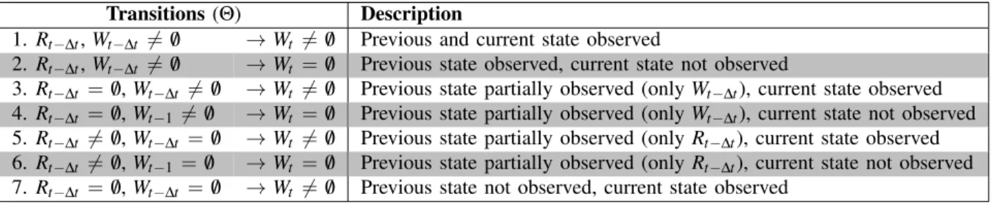
We modeled two possible actions: reading and posting. Therefore, let R be the vector representing what the user read and W the vector representing what the user wrote, then At−∆t ={Rt−∆t,Wt−∆t} and
At={Wt}. In this case NT=7 and table 2 describes the transitions and/or states that can be observed in
the data and that will be used in the simulator. Rt−∆t=/0,Wt−∆t=/0 orWt=/0 represent non-observed data.
Table 2: Description of transitions for two possible actions: read (R) and write (W).
Transitions(Θ) Description
1. Rt−∆t,Wt−∆t 6= /0 →Wt 6= /0 Previous and current state observed
2. Rt−∆t,Wt−∆t 6= /0 →Wt = /0 Previous state observed, current state not observed
3. Rt−∆t = /0,Wt−∆t 6= /0 →Wt 6= /0 Previous state partially observed (onlyWt−∆t), current state observed
4. Rt−∆t = /0,Wt−16= /0 →Wt = /0 Previous state partially observed (onlyWt−∆t), current state not observed
5. Rt−∆t 6= /0,Wt−∆t = /0 →Wt 6= /0 Previous state partially observed (onlyRt−∆t), current state observed
6. Rt−∆t 6= /0,Wt−1= /0 →Wt = /0 Previous state partially observed (onlyRt−∆t), current state not observed
7. Rt−∆t = /0,Wt−∆t = /0 →Wt 6= /0 Previous state not observed, current state observed
Therefore, for instance, suppose a user posted a message aboutObamaand aboutOther topics in the previous ∆t time interval and there are only these two topics being observed; if the first position of the vector is forObama index, and the other forOther in that order; thenWt−∆t= [1,1].
5.1.2 Learning the users behavior
We compute the Maximum Likelihood Estimation (MLE) with smoothing to estimate the parameter for eachθi∈Θtransition type. Therefore, for each user’s sampled data uwe estimateL for:
L(θ|Rt−∆t,Wt−∆t,Wt) =
count(θ,Rt−∆t,Wt−∆t,Wt) +1
count(Rt−∆t,Wt−∆t,Wt) +|S|
(2)
• Non-observed transitionsθ2, θ4,θ6 andθ7:
L(θ|Rt−∆t,Wt−∆t,Wt) =
1
count(Rt−∆t,Wt−∆t,Wt) +|S|
(3)
Where|S|is the number of states.
Recalling that we took into account that the user may post a message related to a topic, which is stored in the setΞ. For this reason, the aforementioned transitions are computed for each topicξi∈Ξ, so that the
actions of the users are modeled according to the type of messages that he/she is reading or writing. Users of OSN usually behave differently according to the period of the day. Therefore, we compute the probability of posting a message at a given period φi∈Φ, where 1≤i≤K. This takes into account
the total of messages mi posted by the user at φi and the messages posted over all periods (the whole
day), as illustrated in equation 4. In addition, we consider the following notation for each periodφi. The
corresponding starting time is denoted φi0∈Φ0, and its length (in hours) is denoted|φi|.
L(posting|φi) = mi
∑
φj∈Φ mj (4)The volume of messages posted by the user is saved in a vector containing integer values, where each position corresponds to the average number of messages written for an element in the setΞ. Equation 5 describes how to compute the transitions volume, given that N represents how manyWt vectors there are
for the same θ transition, L denotes the total of topics, i.e. |Ξ|, and wl j corresponds to the number of
messages written forξl∈Ξand transitionθ.
VWt(θ) = [ ∑j∈Nw1j N , ∑j∈Nw2j N , . . . , ∑j∈NwL j N ] (5)
Volume vectors are computed for both transitions and periods. Equation 6 shows how to compute the average for periods:
V(φi) = [ ∑j∈Mw01j M , ∑j∈Mw02j M , . . . , ∑j∈Mw0L j M ] (6)
Where M represents how many different vectors there are for period φi, and w0l j corresponds to the
number of messages sent for the topicξl ∈Ξat a periodφi.
The volume vectorV(φi), as we will explain further, is used by the simulator to set different weights to
VWt(θ), according to the current periodφi. For this reason, we divide each position ofV(φi) by the mean observed volume over all periods. As a consequence, the periods where the user posted a larger volume of messages will have greater weights than the periods where he/she posted less messages. In equation 7 we demonstrate how this division is done.
V0(φi) = [ v1i ¯ v1j|φj∈Φ , v2i ¯ v2j|φj∈Φ , . . . , vLi ¯ vL j|φj∈Φ ]|vli∈V(φi) (7)
Wherevli denotes the volume for the topicξl and periodφi.
Note that other aspects might be important to better represent the behavior of each user. The first aspect represents the probability of sending a message at a given weekday. The second one is the probability of observing a given lag during the transition between two states. A preliminary evaluation of both have not resulted in a positive impact in the overall modeling the users, and for this reason they are not considered in this work. But we believe that if more data is available, these aspects are worthy of further investigation.
5.2 SMSim Implementation
Considering that the user behavior is modeled into which we can call now theUserModelstructure. During the SMSim initialization two important steps are performed: (i) the graph is loaded from the edges list file; and (ii) for each user in the graph, an agent instance is created and each UserModel file is deserialized into the agent model.
We implemented SMSim using Java and the second step is performed by translating the transitions saved in the UserModel by the modeler to a map where the key represents the source state id and the value is another map containing the probabilities to go from the source state id to the target state id, i.e., the key of the latter map is the target state id and the value is theSimTransitionwhich contains the set of probability values. We defined these maps indexed by the states id to improve performance. Since each agent will have a set of transitions and there will be thousands of agents in the system interacting at the same time.
Every agent (user) is initialized in theIdlestate. When the SMSim is started, each agent switches its behavior toPostingorIdledepending on the activated transitions using Monte Carlo method. The transition will only be activated if the probability value calculated as described in equation 8 corresponds to a random value generated by the system.
ρ(θi) =L(θi|Rt−1,Wt−1,Wt)∗L(posting|φi) (8)
Wherevwt ∈VWt.
In this case, once transitionθi is picked, the volume of messages to be posted for each topicξl in the
periodφi of current time step is calculated using the weighted value of the corresponding average volume:
v(θ,φi,ξl) =vwt(θi)∗v 0
li(φi) (9)
If no transition is activated, the system switches the user’s state toIdle. We performed some experiments where instead of switching the state toIdlewe switched to the most probable state according to the transitions Θ. However that approach did not result in a positive impact in the overall simulation results. The same happened if we create a uniform probability distribution for transitions where both previous and current state were not observed.
5.3 Computing the Engagement Degree Ranking
At each time stept of the simulation the engagement degree of each useruis computed as the following: EDu(tn) =
np(tn)
nr(tn)
(10)
Wherenp andnr are the number of propagated and received messages, respectively, in a give time step tn. Then, when all agents have been stepped in the current time steptn and before transitioning to the next
time step, for each useruthe ranking is computed by: (i) updating the average ofEDufromt=1 tot=n;
(ii) updating the frequency that theEDu fromt=1 tot=nis higher than 0; (iii) generating a coefficient
by multiplying the ranking positions of the average and frequency lists; and finally, (iv) sorting the list users coefficient by the decrescent order.
5.4 Validation
The Root Mean Square Error (RMSE) is frequently used to validate simulation models like weather predictions or to evaluate the differences between two time series. The proposed models are validated using the Coefficient of Variation of the Root Mean Square ErrorCVRMSE (equation 11), where the results of the
simulator are compared with those computed from the observed data. HenceRMSE is applied to compare the curve of the total of messages sent by the users in the simulator, up to a timeT, with the curve plotted
from the observed data used to estimate the parameters of the simulator; and theCVRMSE normalizes to
the mean of the observed data. With this metrics we can compare both pattern and volume. The formula to calculate this error is presented in equation 11.
CVRMSE(T) = q ∑Tt=1(y0t−yt)2 T ¯ y|T t=1 (11)
where y0t represents the total of messages sent in the simulator at timet, and yt denotes the total of
messages sent at timetin the observed data. 6 EXPERIMENTAL RESULTS
In this section we present the experiments conducted with two main goals: a) to validate the modeling approach; and b) to conduct a sensitive analysis aiming at finding the impact of users that are the most likely to disseminate information through the network.
6.1 Scenarios
In order to compare two modeler’s version we change theΦ and|φi|period parameters with regard to the
size and two scenarios are considered:
Fixed: Modeler with 4 periods with equal durations: all periodsΦ=(‘Night’,‘Morning’, ‘Afternoon’, ‘Evening’) have the same length of hours, i.e. |φi|=6,∀φi∈Φ, with the corresponding starting times defined asΦ0=(12:00AM, 6:00AM, 12:00PM, 6:00PM).
Short Night: Modeler with 4 periods and short night: the same 4 periods in Φas the other scenario, but the ‘Night’ period is shorter with a duration of 4 hours and a later starting time, and the other periods are shifted. In addition, both the ‘Afternoon’ and ‘Evening’ periods are 7 hours long and the ‘Morning’ period is 6 hours long. The corresponding starting times are defined asΦ0=(4:00AM, 8:00AM, 2:00PM, 9:00PM). This scenario was defined because: a) the time considered in this work is UTC-3, i.e. Brasilia-Brazil local time, while most users reside in the USA so that the minimum time zone is 3 hours (considering the daylight saving time in both countries); and b) we observed that the volume of messages in the ‘Night’ period (considering the other scenario and the sampled data) generally has a shorter peak than the other scenarios, so the duration of the period should be adjusted.
For both scenarios,∆t=15 minutes. 6.2 Results on Validation
For each scenario we run 10 simulation trials and computed the average. In figure 1(a) the curves representing the volume of messages sent at each simulation step, for both scenarios, are shown along with the volume of messages plotted from the sampled data. In both scenarios the volume of messages results in a curve whose shape is similar to that computed from the real data. In figure 1(b) we show the validation with CVRMSE as described in section 5.4. It can be observed that the error rate of the simulator in the ‘Short
Night’ scenario is generally lower than in the ‘Fixed’ scenario. This indicates that the proper setting of the length and the starting times of the periods may improve the overall modeling of the users’ behavior.
6.3 Sensitive Analysis on Information Propagation
In order to measure the influence around the topics, we discuss the impact on the volume of messages sent through the simulated network by removing important users from it. Because the ‘Short Night’ scenario resulted in a better accuracy, we performed sensitive analysis on the users simulation models estimated
0 100 200 300 400 500 600 200 400 600 800 1000 Messages sent Time step Sampled Fixed Short Night (a) 0 100 200 300 400 500 600 0.0 0.1 0.2 0.3 0.4 0.5 0.6 0.7 Time step Fixed Short Night (b)
Figure 1: The volume of messages per time step in (a), and theCVRMSE validation metric in (b).
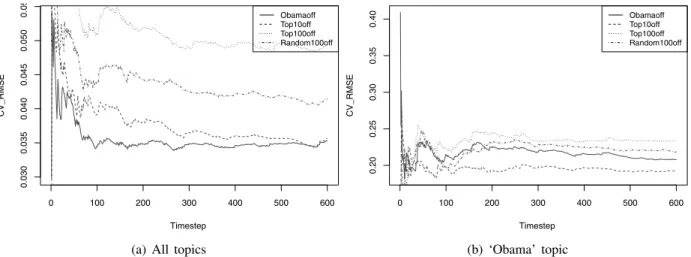
with that scenario. The impact is measured with RMSE andCVRMSE (see section 5.4). In figs. 2(a) and
2(b) we present these results for both the total number of messages for all topics and for ‘Obama’ topic, respectively. 0 100 200 300 400 500 600 0.030 0.035 0.040 0.045 0.050 0.055 CV_RMSE Time step Obama off Top10 off Top100 off Random100 off
(a) All topics
0 100 200 300 400 500 600 0.20 0.25 0.30 0.35 0.40 CV_RMSE Time step Obama off Top10 off Top100 off Random100 off (b) ‘Obama’ topic
Figure 2: Total number of messages for the ‘Short Night‘ simulation scenario.
‘Obama off’ means that the agent representing the Obama’s behavior is inactive in the network. ‘Top10 off’ and ‘Top100 off’ mean that the top 10 and top 100 influencers are inactive in the network, respectively. And ‘Random100 off’ means that 100 users randomly selected are inactive in the network. Recall that Obama is the seed of an egocentric network and his influence impacts more than a set of agents that are not influencers. And finally we want to analyze their impact to test the hypothesis we previously stated: Hypothesis 1: When the seed of the network is inactive, the influence spread by the seed drops considerably. Hypothesis 2: When the top N most engaged users that are also direct seed’s followers are inactive, the influence spread by them drops considerably.
From figure 2(a) we can observe two things: first that the Obama’s influence on the overall number of messages regardless the topic is lower than the inactivation of the others top influencers or inactivation of the random picked users; and second that their overall influence is less than 1 message per time step on average. On the other hand, in figure 2(b) we can see that the impact on the volume of messages about Obama is much higher with an increase of 22% on average. Moreover, Obama has more influence than the
top 10 influencers but less than the top 100 influencers and random 100 users, over time. And the Top100 series dominates the others. From these experiments, both hypothesis were observed in the results.
7 FINAL REMARKS
In this paper we proposed a method to simulate the behavior of users in a social media network, focused on Barack Obama’s Twitter network. The data sampled from Twitter allowed us to build individual stochastic models to represent how each user behaves when posting messages related to Barack Obama or other topics. Experiments considering two different scenarios demonstrated that by removing the seed of an egocentric network or the top most engaged users do impact on the volume of messages, in particular if regarding the topic about the seed. While by removing the top 100 most engaged have more impact than the seed. And by impact we mean it affects consistent and over time the number of messages sent by the users.
As future work, one focus might be improving the methodology employed to better fit the simulator outcome. In addition, others engagement degree computations can be used to find the top engaged users and evaluate their impact in the information flow. It would be also important to evaluate other methods to find the influential users. One direction for this would be to use a search algorithm, in which we could measure the impact of the removal of the users using metrics computed with the simulator.
REFERENCES
Ahn, Y.-Y., S. Han, H. Kwak, S. Moon, and H. Jeong. 2007. “Analysis of topological characteristics of huge online social networking services”. InProceedings of the 16th international conference on World Wide Web, WWW ’07, 835–844. New York, NY, USA: ACM.
Bachrach, Y., M. Kosinski, T. Graepel, P. Kohli, and D. Stillwell. 2012. “Personality and patterns of Facebook usage”. InProceedings of the 3rd Annual ACM Web Science Conference, WebSci ’12, 24–32. New York, NY, USA: ACM.
Bonchi, F., C. Castillo, A. Gionis, and A. Jaimes. 2011, May. “Social Network Analysis and Mining for Business Applications”. ACM Trans. Intell. Syst. Technol.2 (3): 22:1–22:37.
Cha, M., A. Mislove, and K. P. Gummadi. 2009. “A measurement-driven analysis of information propagation in the flickr social network”. InProceedings of the 18th international conference on World wide web, WWW ’09, 721–730. New York, NY, USA: ACM.
Delre, S. A., W. Jager, and M. A. Janssen. 2007, June. “Diffusion dynamics in small-world networks with heterogeneous consumers”.Comput. Math. Organ. Theory13 (2): 185–202.
Fishman, G. S. 2001. Discrete-event simulation: modeling, programming, and analysis. Springer Verlag New York Inc.
Goyal, A., F. Bonchi, and L. V. Lakshmanan. 2010. “Learning influence probabilities in social networks”. In Proceedings of the third ACM international conference on Web search and data mining, WSDM ’10, 241–250. New York, NY, USA: ACM.
Gruhl, D., R. Guha, D. Liben-Nowell, and A. Tomkins. 2004. “Information diffusion through blogspace”. InProceedings of the 13th international conference on World Wide Web, WWW ’04, 491–501. New York, NY, USA: ACM.
Holley, R. A., and T. M. Liggett. 1975. “Ergodic Theorems for Weakly Interacting Infinite Systems and the Voter Model”.The Annals of Probability3 (4): 643–663.
Janssen, M. A., and W. Jager. 2003, September. “Simulating market dynamics: interactions between consumer psychology and social networks”.Artif. Life9 (4): 343–356.
Jennings, N. R. 2001, April. “An agent-based approach for building complex software systems”.Commun. ACM 44 (4): 35–41.
Kempe, D., J. Kleinberg, and E. Tardos. 2003. “Maximizing the spread of influence through a social network”. InProceedings of the ninth ACM SIGKDD international conference on Knowledge discovery and data mining, KDD ’03, 137–146. New York, NY, USA: ACM.
Kwak, H., C. Lee, H. Park, and S. Moon. 2010. “What is Twitter, a social network or a news media?”. InProceedings of the 19th international conference on World wide web, WWW ’10, 591–600. New York, NY, USA: ACM.
Lee, S. H., P.-J. Kim, and H. Jeong. 2009, November. “Statistical properties of sampled networks”.Physical Review E 73.
Leskovec, J., L. A. Adamic, and B. A. Huberman. 2006. “The dynamics of viral marketing”. InProceedings of the 7th ACM conference on Electronic commerce, EC ’06, 228–237. New York, NY, USA: ACM. Leskovec, J., and E. Horvitz. 2008. “Planetary-scale views on a large instant-messaging network”. In
Proceedings of the 17th international conference on World Wide Web, WWW ’08, 915–924. New York, NY, USA: ACM.
Liu, D., and X. Chen. 2011. “Rumor Propagation in Online Social Networks Like Twitter – A Simula-tion Study”. InMultimedia Information Networking and Security (MINES), 2011 Third International Conference on, 278–282.
Macal, C. M., and M. J. North. 2010. “Tutorial on Agent-Based Modelling and Simulation”. Journal of Simulation4:151–162.
Milgram, S. 1967. “The Small World Problem”.Psychology Today2:60–67.
Rogers, E. M., and E. Rogers. 2003, August.Diffusion of Innovations, 5th Edition. 5th ed. Free Press. Saito, K., R. Nakano, and M. Kimura. 2008. “Prediction of Information Diffusion Probabilities for
Inde-pendent Cascade Model”. In Proceedings of the 12th international conference on Knowledge-Based Intelligent Information and Engineering Systems, Part III, KES ’08, 67–75. Berlin, Heidelberg: Springer-Verlag.
Strang, D., and S. A. Soule. 1998. “Diffusion in Organizations and Social Movements: From Hybrid Corn to Poison Pills”.Annual Review of Sociology 24 (1): 265–290.
Wicker, A. W., and J. Doyle. 2012. “Leveraging multiple mechanisms for information propagation”. In Proceedings of the 10th international conference on Advanced Agent Technology, AAMAS’11, 1–2. Berlin, Heidelberg: Springer-Verlag.
AUTHOR BIOGRAPHIES
MAIRA GATTIis a Research Staff Member in the Service Science group at IBM Research-Brazil. Her main area of expertise is in Computer Science and her interests are in Distributed Systems and Multi-Agent-based Simulation. Her email address [email protected].
ANA PAULA APPELhas a PhD in Computer Science from University of S˜ao Paulo and work as a researcher with human data analyses since 2012 at IBM Research-Brazil. Her email address [email protected].
CICERO NOGUEIRA is a Research Staff Member at IBM Research-Brazil since March 2012. His current research focus is on machine learning and data mining approaches. His email address is [email protected].
CLAUDIO PINHANEZleads the Service Systems Research group of IBM Research-Brazil, working on Social Computing, Service Science, and Human-Computer Interfaces. Claudio got his PhD. in 1999 from the MIT Media Laboratory. His email address [email protected].
PAULO CAVALINjoined IBM Research-Brazil in 2012, where he is currently a Research Staff Member. His main research fields are Pattern Recognition/Machine Learning. His email address [email protected].
SAMUEL BARBOSA is a Ph.D. candidate at University of S˜ao Paulo who is currently working as an intern at IBM Research-Brazil, where he develops his thesis on social networks user behavior modelling. His email address [email protected].