Local sensitivity analysis and bias model selection

(1)

Model Selection

Peng Yin

School of Mathematics and Statistics

University of Newcastle upon Tyne

A thesis submitted for the degree of

Doctor of Philosophy

(2)

I would like to thank my supervisor Dr. Jian Qing Shi for valuable guid-ance and advice, and for introducing me to the postgraduate study in the UK and inspiring me in the long but joyful doctoral journey. Thanks are due for his support, encouragement, and patience, which more than fulfilled the requirements of a supervisor role.

Thanks to my colleagues in the School of Mathematics and Statistics, and other peoples in the statistics group for sharing the knowledge and good times. I would also like to acknowledge the School of Mathematics and Statistics at Newcastle University for their financial support.

Thanks to Prof. Jane Hutton and Dr. Malcolm Farrow for being my thesis examiners and providing valuable suggestions and corrections. I am grateful to my family, mum and girlfriend, for their endless love and support, and my best friends who have provided unwavering faith in me.

(3)

Incomplete data analysis is often considered with other problems such as model uncertainty or non-identifiability. In this thesis I will use the idea of the local sensitivity analysis to address problems under both ignorable and non-ignorable missing data assumptions. One problem with ignor-able missing data is the uncertainty for covariate density. At the mean time, the misspecification for the missing data mechanism may happen as well. Incomplete data biases are then caused by different sources and we aim to evaluate these biases and interpret them via bias parameters. Under non-ignorable missing data, the bias analysis can also be applied to analyse the difference from ignorability, and the missing data mechanism misspecification will be our primary interest in this case. Monte Carlo sensitivity analysis is proposed and developed to make bias model selec-tion. This method combines the idea of conventional sensitivity analysis and Bayesian sensitivity analysis, with the imputation procedure and the bootstrap method used to simulate the incomplete dataset. The selection of bias models is based on the measure of the observation dataset and the simulated incomplete dataset by using K nearest neighbour distance. We further discuss the non-ignorable missing data problem under a selection model, with our developed sensitivity analysis method used to identify the bias parameters in the missing data mechanism. Finally, we discuss ro-bust confidence intervals in meta-regression models with publication bias and missing confounder.

(4)

1 Introduction 1

1.1 Missing Data Mechanism . . . 2

1.2 Missing Data Methods . . . 4

1.2.1 Complete Case Analysis . . . 4

1.2.2 Likelihood-Based Approach: EM Algorithm . . . 5

1.2.3 Imputation Procedures . . . 7

1.3 Model Uncertainty and Sensitivity Analysis . . . 10

1.3.1 Local Sensitivity Analysis . . . 11

1.3.2 Bias Model and Bayesian Sensitivity Analysis . . . 11

1.3.3 Missing Data Mechanism Bias . . . 13

1.4 Dissimilarity . . . 14

1.4.1 Nearest Neighbour Distance . . . 17

1.4.2 Permutation Test . . . 20

1.5 Structure of the Thesis . . . 22

2 Local Sensitivity Analysis for Missing Covariates Problems 24 2.1 Introduction . . . 24

2.1.1 Missing Data Problem . . . 25

2.2 Model Uncertainty and Incomplete-Data Bias . . . 25

2.2.1 Linear Model with Missing Confounder . . . 28

2.3 Partially Missing Confounder under MCAR . . . 29

2.3.1 Bias Models . . . 29

2.3.2 Incomplete Data Bias . . . 32

2.4 Partially Missing Confounder under MAR . . . 35

2.4.1 Incomplete Data Bias . . . 36

2.4.2 Simulation Study . . . 38

(5)

2.5.1 Incomplete Data Bias Analysis . . . 42 2.5.2 Simulation Study . . . 45 2.6 Discussion . . . 46 2.7 Appendix . . . 48 2.7.1 Proof of Lemma 2.1 . . . 48 2.7.2 Proof of Lemma 2.2 . . . 49

2.7.3 Proof of the Marginal Model . . . 52

2.7.4 Proof of Theorem 2.1 . . . 53

2.7.5 Proof of Incomplete Data Bias for GLMs under MAR . . . 54

3 Local Sensitivity Analysis for Misspecified Missing Data Mecha-nism 58 3.1 Introduction . . . 58

3.1.1 Uncertainty Problems for MDM . . . 59

3.2 Bias Models with Misspecified MDM . . . 60

3.3 Incomplete Data Bias . . . 63

3.4 Fuel Consumption Data Example . . . 65

3.5 Numerical Results under Misspecified MDM . . . 70

3.5.1 An Example: MAR-MCAR . . . 70

3.5.2 Misspecified MDM Model under MAR . . . 72

3.6 Discussion . . . 75

3.7 Appendix . . . 76

3.7.1 Proof of Theorem 3.1 . . . 76

3.7.2 Fuel Consumption Data . . . 79

3.7.3 Simulation Studies for Complex Misspecified Models . . . 80

4 Monte Carlo Sensitivity Analysis and Selection of Bias Models 85 4.1 Introduction . . . 85

4.2 Monte Carlo Sensitivity Analysis and Bias Model Selection . . . 86

4.2.1 Sensitivity Analysis and Bias Parameter . . . 86

4.2.2 Bias Model Selection . . . 88

4.2.3 Hypothesis Test forη . . . 91

4.3 Numerical Result . . . 92

4.3.1 An Example . . . 92

4.3.2 More Simulation Studies . . . 96

4.4 Monte Carlo Sensitivity Analysis for Fuel Consumption Data . . . 98

(6)

4.6 Appendix . . . 103

4.6.1 K Nearest Neighbour . . . 103

5 Local Bias Analysis for Non-Ignorable Missing Data 105 5.1 Introduction . . . 105

5.2 Bias Analysis for MNAR . . . 107

5.2.1 Double Misspecified Models . . . 107

5.2.2 Triple Misspecified Models . . . 108

5.3 Inference about MDM Bias . . . 110

5.4 Numeric Result for GLMs . . . 114

5.4.1 Equine Data Example . . . 114

5.6 Appendix . . . 117

5.6.1 Model Selection of Covariate Distribution . . . 117

5.6.2 Simulation Studies for Complex MNAR models . . . 119

6 Bias Model Selection for Non-Ignorable Missing Data 125 6.1 Introduction . . . 125

6.2 Mean Estimation with Non-Ignorable Missing Data . . . 126

6.3 Regression Models with Non-Ignorable Missing Data . . . 129

6.3.1 Fuel Consumption Data Example . . . 131

6.3.2 Simulation Studies for Misspecified Models . . . 134

6.5 Appendix . . . 137

6.5.1 Proof of Lemma 6.1 . . . 137

6.5.2 BSA Details used in Section 6.3.1 . . . 138

7 Robust Confidence Interval with Missing Data in Meta Analysis 139 7.1 Introduction . . . 139

7.2 Meta Regression Model and Confidence Intervals . . . 140

7.3 Extension of HC methods . . . 144

7.3.1 Trend Estimation in Meta-Analysis . . . 144

7.3.2 Bootstrap Methods (BS) . . . 147

7.4 Simulation Study with Publication Bias . . . 148

(7)

7.4.2 Confidence Intervals with Publication Bias . . . 150

7.5 Missing Confounder Problems in Meta-Analysis . . . 150

7.7 Appendix . . . 154

7.7.1 Proof of Equation (7.6) . . . 154

7.7.2 Proof of Equation (7.19) . . . 157

8 Conclusions and Future Work 162

(8)

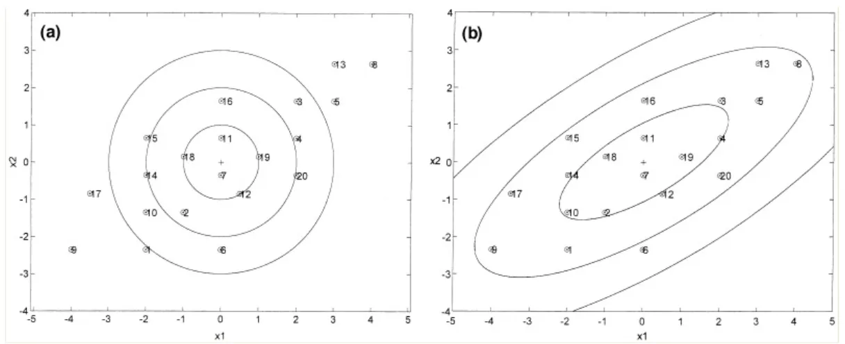
1.1 Euclidean and Mahalanobis distance illustration. (a) Plot of the sim-ulated data for two variables x1 and x2 together with the circles rep-resenting equal Euclidean distances towards the centre point; (b) Plot of the simulated data for two variables x1 and x2 together with the ellipses representing equal Mahalanobis distances towards the centre

point. . . 17

1.2 Examples of three inter-cluster distance measures: single, complete and average . . . 18

2.1 Curves h(r = 1|x) for various MDM models. Black line: MCAR with h(r = 1) = expit(1); Blue: MAR with h(r = 1|x) = expit(1−0.1x); Grey: MAR with h(r = 1|x) = expit(1−x); Red: MAR with h(r = 1|x) = expit(1−3x). . . 40

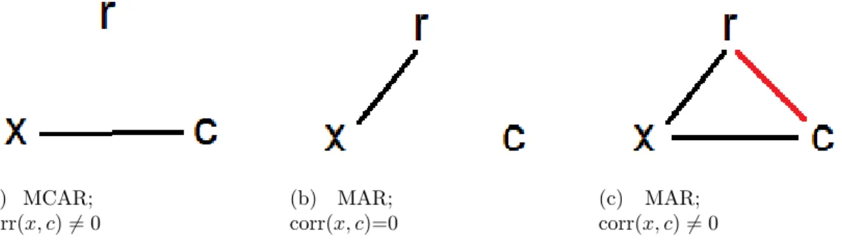
2.2 Picture of relationship between missingness indicatorR with covariate variables X and C. . . 40

3.1 Bias models with misspecifications. . . 61

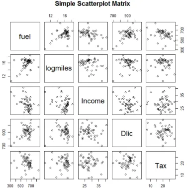
3.2 Scatterplot matrix for fuel consumption data . . . 66

3.3 Estimation of correlations. . . 69

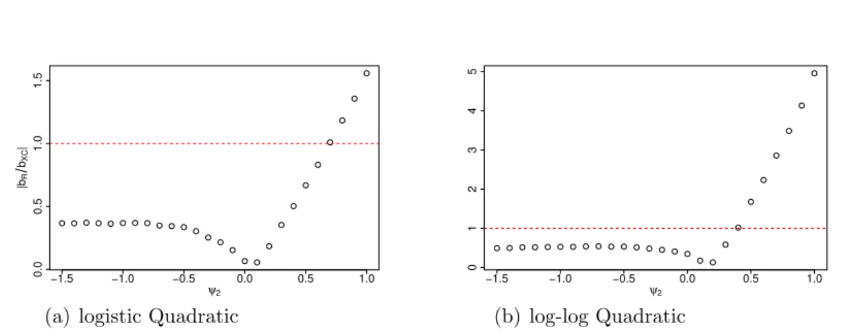
3.4 Simulation study: ratio of missing data bias and covariate bias. ψ2 ∈ (−1.5,1). . . 75

4.1 Diagram of bias model . . . 89

4.2 Selection of corr(x, c) under hierarchical measure. . . 94

4.3 Selection of corr(x, c) under KNN measure. Upper panel use Euclidean metric and lower panel use Mahalanobis metric. . . 95

(9)

4.5 Contour plots for selection of corr(x1, x2) and corr(x2, x3) for fuel con-sumption data. Fig (a): distance; Fig (b): achieved significance level. Mahalanobis average distance is used as in MC-BMS method. . . 101 5.1 Selection of corr(x, c). . . 118 5.2 Achieved significance level . . . 119 6.1 Bias parameter selection. Upper panel: KNN distances versus

differ-ent values of ψ; Lower panel: KNN distance versus the corresponding estimate of µfor the given value of ψ. . . 128 6.2 Bias parameter selection: histograms of the selected ψ with different

MC sizes. . . 130 6.3 Selection of bias parameter ψ for fuel consumption data: KNN (K=2)

distance versus values of ψ. . . 133 7.1 Coverage probabilities of the confidence intervals without assuming

publication bias. The dotted line stands for the 95% nominal proba-bility. . . 149 7.2 Coverage probabilities of the confidence intervals under the moderate

publication bias (γ = 3). . . 151 7.3 Coverage probabilities of the confidence intervals under the strong

pub-lication bias (γ = 1.5). . . 152 7.4 Biases of the fixed-effects and random-effects estimates under moderate

and strong publication bias: (a)(b) with moderate publication bias (γ = 3); (c)(d) with strong publication bias (γ = 1.5). . . 153 7.5 Coverage probabilities of the confidence intervals with moderate

cor-related missing confounder. . . 154 7.6 Coverage probabilities of the confidence intervals with strong correlated

(10)

1.1 Dissimilarity measures for continuous data. . . 16

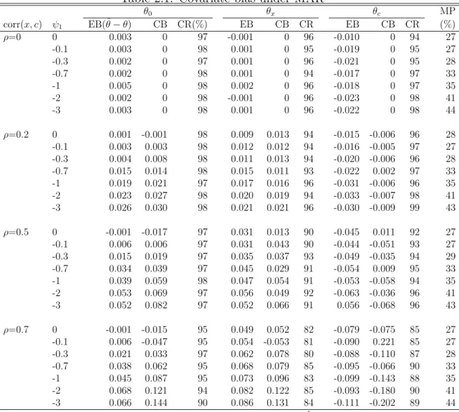
2.1 Covariate bias under MAR . . . 41

2.2 Covariate bias for GLM under MAR . . . 47

3.1 Variables in fuel consumption data . . . 65

3.2 Correlation of covariates in fuel consumption data . . . 65

3.3 Simulation study result . . . 67

3.4 Parameter estimation for conditional covariate density . . . 68

3.5 Covariate bias and MDM bias . . . 73

3.6 MAR simulation 1 . . . 82

4.1 Sensitivity analysis results of selecting corr(x, c) . . . 96

4.2 Sensitivity analysis and selection of corr(x, c) by MC-BMS . . . 99

4.3 Simulation results with covariate density uncertainty . . . 102

5.1 Simulation results for ˆθ . . . 113

5.2 Bias analysis result for Equine data under MNAR . . . 114

5.3 Incomplete data biases for GLM under MNAR . . . 116

5.4 Sensitivity analysis results . . . 118

5.5 MNAR simulation 1 . . . 121 5.6 MNAR simulation 2 . . . 121 5.7 MNAR simulation 3 . . . 122 5.8 MNAR simulation 4 . . . 122 5.9 MNAR simulation 5 . . . 123 5.10 MNAR simulation 6 . . . 123

(11)

6.1 Bias model selection: simulation study . . . 129 6.2 Simulation study for fuel consumption data . . . 133 6.3 Simulation study: average estimates and RMSE (in brackets) . . . 135 7.1 Coverage probabilities without publication bias (τ2 _{= 0}_.₅_×₁₀−4₎ _{. .} ₁₄₉

(12)

Introduction

Problems ofmodel uncertainty andincomplete data arise frequently in the statistical sciences. Most of the literature usually assumes that the model is correct and that we obtain observations on the variables that are described by that model: we have model certainty and complete data. In reality model certainty is always doubtful and incomplete sets of data are common.

Much of the theory and practice of statistics involves fitting parametric models for missing data, which comprises two components: one is for the complete data and the other is for the missing data mechanism (MDM). The former describes the probability distributions that fit the observations on the variables, while the latter characterizes the observation process by which some data may be missing or censored. We will first review the missing data types in Section 1.1. When we assume model certainty, many statistical techniques can be used to specify parametric models with missing data and we will review some of most popular methods in Section 1.2. Next the model uncertainty analysis will be addressed, and local bias analysis and sensitivity analysis will be discussed in Section 1.3. Since we will develop a novel approach of sensitivity analysis and make bias model selection by comparing the observed data set and a simulated data set, the choice of dissimilarities is important and the distance measures are reviewed in Section 1.4. Hypothesis testing is also considered and the procedure of permutation test is described. In Section 1.5, we will outline the structure of the thesis.

(13)

1.1

Missing Data Mechanism

Little and Rubin (2002) characterize the missing data mechanism into three types generally: missing completely at random (MCAR), missing at random (MAR) and missing not at random (MNAR). The first two missing types are usually considered as ignorable missing data while the MNAR is then named as non-ignorable missing data. Lu and Copas (2004) gave precise definitions of MAR and likelihood ignorable, and discussed the conditions when both are equivalent.

Suppose we have an-dimensional random vectorZ = (z1, . . . , zn)T and ad-dimensional

parameters of interest θ ∈ Θ. A working model f(z;θ) on z ∈ _Rn _{can be assumed}

for inference. Suppose that the observation process of Z suffers from missing data and hence, we need to define a binary random vector R = (r1, . . . , rn)T indicating

the observational status of Z, where ri takes the value 0 when the observation of zi

is missing and the value 1 whenzi is observed, i= 1, . . . , n.

ri =    1, zi observed; 0, zi missing. (1.1)

The parameterization of the joint distribution ofZ and Rcan always be fitted by the selection model form

f(z, r;θ, ψ) = f(z;θ)f(r|z, ψ), (θ, ψ)∈Θ×Ψ, (1.2)

with the parameters θ and ψ are assumed to be distinct (Rubin, 1976). The item f(z;θ) fits the probability density of the observations while the conditional density f(r|z, ψ) characterizes the missingness process on the observations and thus specifies a model for the missing data mechanism. The pair of random variables (Z, R) induces an observable random variable Y, which is

Y =Y(Z, R) = (y1, . . . , yn)T. (1.3) where yi =    zi, ifri=1; R, ifri=0. i= 1, . . . , n.

(14)

where the symbol _R used in the vector argument means when r = 0 all we know is that the missing values are distributed at some points in _R = (−∞,−∞). In this case, complete dataZ can be separated into two components: the set of the observed values Zobs and the set of the missing values Zmis. 1 The density of incomplete data Y can be expressed as:

f(y;θ, ψ) = Z (y) f(z;θ)f(r|z;ψ)dz = f(zobs;θ) Z

f(zmis|zobs;θ)f(r|z;ψ)dzmis (1.4)

where (y) on the integration sign means the the marginal density is taken over the level set, i.e. Y = Y(Z, R). Examples of level sets of y(z, r) can be found in Copas and Eguchi (2005, p.463).

Thus Rubin’s MAR condition can be expressed as follows. A MDM is said to be

MAR if the conditional distribution f(r|z;ψ) has the special form (Lu and Copas, 2004)

f(r|z;ψ) = h(y(z, r), ψ) for all (z, r)∈Z×R, (1.5) where, for any fixedψ andr,h(.;ψ) is a function mapping real number field into [0,1]. Under MAR, the MDM depends on y only through the observed part of the sample

y=y(z, r).

Also it is well known that MCAR is a special case of MAR, where Z and R are statistically independent in the usual sense. Rubin (1976) and Little and Rubin (2002) distinguished betweenmissingness completely at random, where the outcomes are independent of the mechanism governing missingness, andmissingness at random, where there is dependence between, but only in the sense that missingness may depend on the observed, but not further on the unobserved measurements. Normally MAR (and MCAR) are named as ignorable in the likelihood setting. Lu and Copas (2004) give the definition of likelihood ignorable (LIG) to explain the meaning of it:

Definition 1. A MDM is said to be LIG if the integral

Z

f(zmis|zobs;θ)f(r|z;ψ)dzmis (1.6)

1_{The complete data}_Z _{can be separated in different ways for different purposes. For example, we} use subscript here to denote a set of the observed values (i.e. Zobs) or missing values (Zmis). Also

in Chapter 6, we use superscript to denote a set of variables which are always observed (Zobs_{), or a}

(15)

is free ofθ for almost all realizations of (z, r)∈Z×R and for all (θ, ψ)∈Θ×Ψ.

And they stated that generally MAR is a necessary and sufficient condition for LIG for complete density family.

When neither MCAR nor MAR hold, we say the data are missing not at random or non-ignorable, which means that even accounting for all the available observed information, the reason for observations being missing still depends on the unseen observations themselves. In this case, it is not always theoretically possible to char-acterize all parameters for this class of models given a certain choice of covariates, and this problem is termed as model non-identifiability.

1.2

Missing Data Methods

Over the last several decades a variety of models and methods are proposed to an-alyze incomplete data. Because standard techniques for regression models require fully observed information, one simple way to avoid the problem of missing data is to infer from the subjects that are completely observed. This method, known as a complete case (CC) analysis, is the technique most commonly used with missing val-ues in the covariates and/or response, although it can be biased except the data are MCAR. Another ad hoc method of dealing with missing covariate data is to exclude those covariate variables with missingness from the analysis. But this procedure can lead to model misspecification (missing confounder) and is not recommended. Other approaches like maximum marginal distribution (MLE with EM algorithm), multiple imputation (MI), fully Bayesian (FB), and weighted estimating equations (WEEs) methods are getting popular for a wide variety of missing data problems, includ-ing missinclud-ing covariate data in the linear regression model, generalized linear models (GLMs), survival analysis, as well as missing responses in the model of longitudinal data and meta analysis.

1.2.1

Complete Case Analysis

One simple way to avoid the missing data problem will be to use complete case anal-ysis, excluding all units for which the outcome or any of the inputs are missing. This method has advantages such as simplicity, and comparability of univariate statistics,

(16)

since these are all calculated on a common sample base of cases. However, this ap-proach may suffer biased estimations as it discards incomplete cases and thus loss some information. Little and Rubin (2002) pointed out that the only unbiased sit-uation is under MCAR assumption, then the complete case is just one effectively random subsample of the original dataset. But in other cases, the analysis without modification will cause seriously biased results and is not recommended.

1.2.2

Likelihood-Based Approach: EM Algorithm

The maximum likelihood method is one of the most popular methods for bias analysis with missing data. Many articles in the literature discuss missing responses and/or missing covariates under ignorable or non-ignorable assumption by this method. These include Little and Rubin (2002), Diggle and Kenward (1994), Ibrahim et al. (2005) and Molenberghs et al. (2008).

Chen and Ibrahim (2001) proposed semiparametric maximum likelihood estimators for identifiable regression coefficients. Under the same identity assumption and with a conditioning argument on MDM, Tang et al. (2003) made inferences based on a pseudo-likelihood function. Subsample ignorable likelihood for regression analysis with missing data has also been discussed by Little and Zhang (2011). Empirical likelihood based inference procedure has been proposed by Rao and Wang (2002) and Qin and Zhang (2007). There has also been some literature for likelihood based methods for establishing identifiability and asymptotic properties of estimators in missing covariate problems such as Robins and Rotnitzky (1995).

Let Dobs and Dmis denote the observed values and missing values respectively. The

marginal probability density of Dobs is obtained by integrating out the missing data

Dmis:

f(Dobs|θ) =

Z

f(Dobs, Dmis|θ)dDmis.

We define the likelihood ofθ based on dataDobs but ignoring the missing-data

mech-anismto be any function of θ proportional to f(Dobs|θ):

L(θ|Dobs)∝f(Dobs|θ).

More generally, we can include in the model the distribution of a variable indicating whether each component of D is observed or missing. Similar to notation (1.1), we

(17)

define an indicator R as follows R =    1, D observed; 0, D missing. (1.7)

We can treat R as a random variable and specify the joint distribution of R and D. The density of this distribution can be specified as the product of the densities of the distribution ofD and the conditional distribution of R given D, that is,

f(D, R|θ, ψ) = f(D|θ)f(R|D, ψ).

The conditional distribution ofR givenDindexed by an unknown parameterψ refers to the model of the missing-data mechanism we introduced. In some situations the distribution is known, andψ is unnecessary. The actual observed data consist of the values of the variables (Dobs, R), and the distribution of the observed data is:

f(Dobs, R|θ, ψ) =

Z

f(Dobs, Dmis|θ)f(R|Dobs, Dmis, ψ)dDmis.

The likelihood of θ and ψ is any function of θ and ψ proportional to the equation above:

L(θ, ψ|Dobs, R)∝f(Dobs, R|θ, ψ).

And if missing data is LIG, then the distribution of observed data is:

f(Dobs, R|θ, ψ) =f(R|Dobs, ψ)f(Dobs|θ).

The Expectation-Maximization(EM) algorithm is a very general iterative algorithm for ML estimation in incomplete-data problems. In fact, the range of problems that can be attacked by EM is very broad and includes problems not usually considered to be ones arising from missing or incomplete data (e.g. variance components estimation, iteratively reweighted least squares). The algorithm is comprised of two steps: an Expectation step and a Maximization step. Specifically, letθ(i)be the current estimate of the parameterθ. The E step of EM finds the expected loglikelihood ifθ wereθ(i)_:

Q(θ|θ(i)) =

Z

(18)

wherel(θ|D) is the log-likelihood ofθ.

The M step of EM determines θ(i+1) _{by maximizing this expected loglikelihood, and} it has the following property:

Q(θ(i+1)|θ(i))≥Q(θ, θ(i)), f or all θ.

The E step calculates the conditional average of the ‘missing data’ given the observed data conditional on the current parameter estimations, and then substitutes these expectations for the ‘missing data’. The quotations around ‘missing data’ are there because the missing values themselves are not necessarily being substituted by EM, which is different from imputation procedure.

The M step is particularly simple to describe: perform maximum likelihood estimation of θ just as if there were no missing data, that is, as if they had been filled in. Thus the M step of EM uses the identical computational methods as ML estimation from l(θ|D). These two steps are then iterated until convergence happens. The stationary point is a global maximum and EM yields the unique maximum likelihood estimate of θ froml(θ, Dobs) in well behaved problems (Schafer, 1997, pages 51-55), i.e. problems

with not too many missing entries and not too many parameters.

1.2.3

Imputation Procedures

Imputation is another general and flexible method for handling missing data problems. There are many ways to make the fill-in, and we list some of the most popular below: 1. Mean imputation: where means from the responding units in the sample are substituted. The idea is to replace each missing value with the mean of the observed values for that variable. Let xij be the value of X for units j in

variablei, i= 1, . . . , m, j= 1, . . . , n. Mean imputation substitutes the mean ¯xi

of theni responding units for units that are sampled but that do not respond: xr_ij=0 = ¯xr_i=1. However, this approach can distort the shape of distributions and then distort relationships between variables.

2. Hot deck imputation: can be broadly defined as a method where an imputed value is selected from an estimated distribution for each missing value, in con-trast with mean imputation, where the mean of the distribution is substituted.

(19)

The simplest theory is obtained when imputed values can be selected from the values for the responding units by a probability sampling design. The hot deck with replacement selects is the most common one, but its estimator is only unbiased under unrealistic assumption that the probability of response is not related to the values ofX. The nearest neighbour hot deck (Sander, 1983) and the sequential hot deck (Colledge et al., 1978) approach may be considered to improve the method.

3. Regression imputation: replaces missing values with predicted values from a regression of the missing item given items observed for the unit, usually calcu-lated from units with both observed and missing variables present. One simple way is to fit a parametric regression model of variables with missingness against variables totally observed, based on observed samples only, then predict the variables with missingness by the regression model (Little and Rubin, 2002). There are many regression technique, such as stochastic regression imputation and Bayesian linear regression imputation. Generally, this method is model based imputation technique and is widely used in multiple imputation meth-ods.

4. Multiple imputation methods(Rubin, 1978, 1987): impute more than one value for the missing items. This method is most widely used now and we have a detailed review below.

Multiple Imputation:

Multiple imputation was first proposed by Rubin (1978) and a comprehensive dis-cussion can be found in Little and Rubin (2002), Schafer (1997) and Raghunathan et al. (2001). The method has valid inference on missing data problem, especially under ignorable missingness assumption and thus has a variety of applications. Single imputation introduced above has the advantage of allowing standard complete data methods of analysis, however, it is also difficult to reflect sampling variability under one model for nonresponse as pointed out by Little and Rubin (2002). While mul-tiple imputation can overcome this problem as the method involveN complete data analyses to display variation in valid inferences across the models in dealing with uncertainty. The analysis of a multiply imputed data set is quite direct. Suppose

(ˆθi, Wi), i = 1, . . . , N are N complete-data estimates and their associated variance

(20)

model. In order to make inferences forθ we average the results across the individual imputations: ¯ θ= 1 N N X i=1 ˆ θi.

The variability associated with the estimate has two components: the within impu-tation variance: W = 1 N X ˆ Wi,

and the between-imputation variance:

B = 1

N−1

X

(ˆθi−θ¯)2

thus the total variability is combined as

V =W + (1 + 1

N)B.

A rough 95% confidence interval can be obtained as ¯θ±2V1/2_{, but a better calculation} is to use the approximation of Student’st distribution:

(θ−θ¯)V−1/2 ∼tν,

with the degrees of freedom,

ν = (N −1)[1 + 1 N + 1 W B] 2 .

Notice that when there is infinite number of imputations (N =∞), the total variance V reduce to the sum of the two variance components, then the confidence interval is based on a normal distribution (ν=∞).

Rubin (1987) pointed out that the efficiency of the estimate based onN imputations of a proportion pof missing data is

(1 + p

N)

−1_,

(21)

As there are various imputation techniques which can be applied in practice, how to make a proper imputation strategy must be considered. MI procedure requires a mechanism and statistical assumptions to make valid inferences. The basic idea is sampling data from a conditional distribution of variables with missingness on variables without missingness. Take the missing covariates problem for example, assume response variables T is completely observed and covariate variables X is partially missing. R is the missingness indicator defined in equation (1.7). Then the imputation distribution is given as

f(xmis|t, xobs, R)∝f(t|x, θ)f(x)f(R|t, x, ψ).

Specially, when the missing data mechanism is assumed under ignorable missingness, the MDM need not to be specified in this case, and the above equation reduces as

f(xmis|t, xobs, R)∝f(t|x, θ)f(x).

1.3

Model Uncertainty and Sensitivity Analysis

An assessment of uncertainty due to incomplete data or model misspecification is a topic that has attracted many researchers for several decades, (see e.g Cornfield et al., 1959; Vemuri et al., 1969; Draper, 1995; Copas and Li, 1997), in which sensitivity analysis is one of the most commonly used approaches. It has been widely used in bias analysis for different areas, including: sensitivity analysis for publication bias in meta-analysis (Copas and Shi, 2000a,b) using the Heckman model (Heckman, 1979), sensitivity analysis for incomplete contingency tables by Molenberghs et al. (2001), local sensitivity analysis in Cook (1986), Copas and Eguchi (2001) and probabilistic sensitivity analysis in Oakley and O’Hagan (2004). Those discussions characterize the sensitivity analysis in different ways, but their aims are essentially the same: to examine the influence of individual uncertainty on model based inference. A different approach is to consider all possible sources of uncertainty by defining a prior density, and a Monte Carlo sensitivity analysis involves sampling ‘bias parameters and then inverts the bias model to provide a distribution of bias-corrected estimates’ (Greenland, 2005, p.269). Also Draper (1995) evaluated the model uncertainty through Bayesian

(22)

model averaging while Saha and Jones (2005) applied the bias analysis techniques to address non-identifiability issues.

1.3.1

Local Sensitivity Analysis

Copas and Eguchi (2005, 2001) discuss local model uncertainty when inference is based on incomplete data. We still use the notation defined in Section 1.1, denoting Zfor complete data andY for incomplete data. The data sampling distribution under complete data is denoted asgZ(z;θ) and its marginal model asgY(y;θ). The working

modelfZ under complete data (which is misspecified fromgZ) has the corresponding

marginal distributionfY under incomplete data, inference based on fY (misspecified

marginal model) θY has a bias from inference from complete data θZ. The bias is

named as incomplete data bias and the models for measuring the bias are called

bias models. However, Lin et al. (2012) found under identifiable assumption, the working model fY is not always the same as the marginal model of fZ, and extra

misspecification occurs. Lin et al. (2012) extended Copas and Eguchi’s work and discussed the so-calledmarginal model bias in missing confounder problem for GLMs with nonlinear link functions. The details of local sensitivity analysis for incomplete data will be discussed in Chapter 2 and 3.

1.3.2

Bias Model and Bayesian Sensitivity Analysis

Sensitivity analysis is mainly used to determine the statistical uncertainty issue in fac-torizingmodelsorparameter errors. Good references about sensitivity analysis about modelling uncertainty include Saltelli et al. (2004), Saltelli et al. (2008) and Oakley and O’Hagan (2004), but in this thesis, we mainly focus on the sensitivity analysis with nuisance parameters in the missing data problem. Let D and R denote the ob-servations vector and missingness indicator vector which takes 1 if data is observed or 0 otherwise. The complete data model can be factorized into an extrapolation model and an observed data model,

f(D, R|θ) =f(Dmis|Dobs, R, θmis)f(Dobs, R|θobs). (1.8)

The observed data distribution f(Dobs, R|θobs) is identifiable and can be fitted by

(23)

f(Dmis|Dobs, R, θmis) cannot be identified unless extra assumptions are made.

Sen-sitivity of non-identifiable parameters should be considered carefully. Those param-eters are therefore described as sensitivity parameters or bias parameters (Daniels and Hogan, 2008; Greenland, 2005), denoted byη. Local sensitivity analysis is based on derivatives of parameters of interest evaluated at some belief η = η0 which helps us to understand the robustness of the practical model in a local area, but has lim-ited value in understanding the consequences of global uncertainty about η. Global sensitivity analysis considers these more substantial changes individually without lim-itation (see e.g. Oakley and O’Hagan, 2004) although an unrealistically wide range is usually a troublesome problem without proper selection on the inputs. Bayesian techniques were then proposed to overcome the difficulty (McCandless et al., 2007, 2008; Gustafson et al., 2010, see e.g.), offering a route to sample smoothly via a prior distribution, and it weights possible scenarios rather than the conventional method which only reflects the investigator’s plausible beliefs. Take one example in Mc-Candless et al. (2007), let T be disease variable, X1 as exposure and X2, C denote the measured and unmeasured confounders respectively. They used the factorization

P(T, C|X1, X2) = P(T|X1, C, X2)P(C|X1, X2) and model the confounding effect of

C using logistic regression models:

logit[P(T = 1|X1, C, X2)] =θ0+θ1X1+θ2C+θ3X2,

logit[P(C = 1|X1, X2)] =η0+η1X1+η2X2.

To interpret the parameter of interest θ = (θ0, θ1, θ2, θ3), we need to specify a joint prior distribution of (θ, η) as f(θ|T, X1, X2, C) = Z f(θ|T, X1, C, X2, η)f(η|T, X1, C, X2)dη ∝ Z P(T, X1, C, X2;θ, η)f(θ, η)dη.

In principal, a prior distributionf(θ, η) from any standard parametric family can be used for Bayesian sensitivity analysis (BSA). In most literatures, priors are usually specified independently as

f(θ, η) =f(θ)f(η) (1.9)

and the exponential family is always a popular choice. However, there is rarely discussions on testing the prior choice on the performance of interval estimators, since

(24)

the sensitivity parameter is unknown. Depending on the specified prior distribution, the posterior average may be asymptotically biased and credible intervals may not have expected coverage probability, according to Gustafson (2005).

Monte Carlo sensitivity analysis (MCSA) is a type of Bayesian sensitivity analysis with modifications. Assuming that f(θ|η) is uniformly distributed and posterior distributionf(η|Dobs, R) is close to the prior distributionf(η), the MCSA procedure

is to sample from f(θ|Dobs, R) = Z f(θ|Dobs, R, η)f(η|Dobs, R)dη ≈ Z f(θ|Dobs, R, η)f(η)dη;

the details can be found in Greenland (2005). However, since

f(η|Dobs, R) ∝

Z

f(Dobs, R|η, θobs)f(θobs|η)f(η)dθobs

=

Z

f(Dobs, R|θobs)f(θobs|η)f(η)dθobs

= f(Dobs, R|η)f(η),

that means the posterior of the bias parameters is not equal to the prior i.e.,f(η|Dobs, R)6= f(η); more discussion can be found in Daniels and Hogan (2008).

1.3.3

Missing Data Mechanism Bias

As well as the totally missing confounder problem, partially missing covariates issue is also very common. The literature analyse the partially missing data in partially linear models such as Liang et al. (2004) , GLMs such as Ibrahim and Lipsitz (1999), survival analysis such as Herring et al. (2004) and longitudinal data study such as Chen and Zhou (2011) etc.

The selection modelgZ =f(Z)f(R|Z) and pattern mixture modelgZ =f(Z|R)f(R)

are two classes of models described by Little(1993,1994) for missing data problems. When the MAR assumption is plausible, the selection model formulation seems com-pelling because it leads to likelihood ignorable for complete density family. However, as pointed out by Little (1993), valid inference is based on knowledge of the missing data mechanism; if assumptions about the missing data mechanism are misspecified, extra uncertainty bias exists and we call it missing data mechanism bias. We will

(25)

consider the model uncertainty under the three types of MDM respectively, and lo-cal bias analysis is conducted under identifiable assumption. And the incomplete data bias is separate, particularly as covariate bias, missing data mechanism bias and marginal model bias (for non-linear models) due to their bias sources. Bias analy-sis under non-ignorable missing data is particularly difficult and we can assume an ignorable working model, then the MDM bias actually measures the departure from non-ignorability. However, the true MDM model is unknown in practice and further sensitivity analysis is required.

Local sensitivity analysis for misspecified MDM will be discussed generally in Chapter 3 and the problems with non-ignorable missing data will be further disscussed in Chapter 5 and 6.

1.4

Dissimilarity

In Chapter 4, we will propose a new method for sensitivity analysis. One key step is to measure the similarity or dissimilarity between the observed data set and a simulated set.

A quantitative measure of closeness is named asdissimilarity, distance or similarity

(a general term is proximity) (Everitt et al., 2011). Gower and Legendre (1986) summarized a list of similarity measures for binary data, and Gower (1971) proposed one general similarity measure to construct proximities for mixed mode data (with continuous and categorical):

sij = p X k=1 wijksijk/ p X k=1 wijk

where sijk is the similarity between the ith and jth individual as measured by the kth variable, and wijk is typically one or zero depending on whether or not the

comparison is considered valid. For binary and categorical variables with more than two categories, the component similarities, sijk, take the value one when the two

individuals have the same value and zero otherwise. For continuous variables, Gower suggests using the similarity measure

(26)

wherexik andxjk are respectively thekth variable value of thep-dimensional

observa-tions for individualsi and j, andRk is the range of observations for the kth variable.

More suggested similarity measures can be found in Estabrook and Rodgers (1966), Legendre and Chodorowski (1977), Lerman (1987) and Ichino and Yaguchi (1994). Dissimilarity measures or distance measures between individuals are typically cal-culated to describe the proximities for continuous variables, where a dissimilarity measure, dij, is termed adistance measure if it fulfills the metric inequality

dij +dim ≥djm

for pairs of individualsij,im and jm(Everitt et al., 2011). Also a series of measure-ment spaces have been proposed for deriving a dissimilarity matrix, such asEuclidean distance,Minkowski distance ,Canberra distance, etc. See Table 1.4. More summary lists can be found in Gower (1985), Gower and Legendre (1986), Jajuga et al. (2003) and Everitt et al. (2011). The most commonly used distance isEuclidean distance

dij = [

p

X

k=1

(xik−xjk)2]1/2,

which is a special case (r = 2) of the Minkowski metric

dij = [

p

X

k=1

(xik−xjk)r]1/r.

This distance can be interpreted as physical distance between two p-dimensional points x0_i = (xi1, . . . , xip) and x0j = (xj1, . . . , xjp) in Euclidean space. It is commonly

used to evaluate the proximity of objects in two or three dimensional space and it works well when a data set has ‘compact’ or ‘isolated’ clusters (Mao and Jain, 1996). Investigations of the relationships between dissimilarity matrices, distance matrices and Euclidean matrices are carried out in Gower and Legendre (1986) and Cailliez and Kuntz (1996). Another widely used distance is Mahalanobis distance, which is scaled space from the Euclidean norm but would reduce into Euclidean norm when covariance matrix shrinks into diagonal. It is given as

dij = [

p

X

k

(27)

Table 1.1: Dissimilarity measures for continuous data. Measure Formula Euclidean distance dij = [ p P k=1 (xik−xjk)2]1/2 Manhattan distance dij = p P k=1 |xik−xjk| Minkowski distance dij = ( p P k=1 |xik−xjk|r)1/r (r ≥1) Canberra distance dij =    0 forxik =xjk=0; p P k=1 |xik−xjk| (|xik|+|xjk|) for xik 6= 0 or xjk 6= 0 Pearson correlation dij = (1−φij)/2 with φij = p P k=1 (xik−x¯i.)(x_jk −x¯_j.)/[ p P k=1 (xik−x¯i.)2 p P k=1 (xjk−x¯j.)2]1/2 where ¯xi. = p P k=1 xik/p Angular separation dij = (1−φij)/2 with φij = p P k=1 xikxjk/[ p P k=1 x2 ik p P k=1 x2 jk]1/2

Mahalanobis distance dij = [(xi−xj)TS−1(xi−xj)]1/2, S is covariance matrix

with S as covariance matrix.

Figure 1.1 (by Maesschalck et al., 2000) presents points with the same inter-cluster Euclidean and Mahalanobis distances from centre points by circles and ellipses respec-tively. The Euclidean distance spread evenly as circles while Mahalanobis distance as ellipses scaled by its covariance matrix, i.e. point 4 has the same distance as point 20 from centre under the Euclidean metric; but point 20 is farther than point 4 under the Mahalanobis metric. However, Mahalanobis space will reduce into Euclidean space if the covariance matrix is diagonal.

(28)

Figure 1.1: Euclidean and Mahalanobis distance illustration. (a) Plot of the simulated data for two variablesx1andx2 together with the circles representing equal Euclidean distances towards the centre point; (b) Plot of the simulated data for two variablesx1 and x2 together with the ellipses representing equal Mahalanobis distances towards the centre point.

1.4.1

Nearest Neighbour Distance

A series of methodologies have been developed since people find the necessity of clus-tering observations into different groups, which include hierarchical and partitional approaches (hierarchical classification consists of a series of partitions while partitional methods produce only one). There is literature that summarizes these methodologies such as Jain and Dubes (1988), and Jain et al. (1999) and Everitt et al. (2011).

Hierarchical Clustering:

Everitt et al. (2011) pointed out that hierarchical clustering techniques may be sub-divided into agglomerative methods, which begin with each pattern in a singleton cluster and merge clusters together, and divisive methods which separate the whole cluster (observations) into finer groupings. Most popular heuristic clustering criteria includesingle linkage (nearest neighbour),complete linkage (farthest neighbour) and

average linkage. The single link was first introduced by Florek et al. (1951) and later by Sneath (1957) and Johnson (1967). It is also known as the nearest neighbour technique, but if not only the one closest individual defined as its neighbour, but kth nearest are chosen as neighbours, we call it kth Nearest Neighbour. Complete linkage is the opposite of single linkage, and the defining feature is that the distance between groups is that of the most distant pair of individuals. Average linkage - the distance between all pairs of individuals from each group or weighted average linkage

(29)

(McQuitty, 1966) works well in clustering, and these methods are compared in lots of studies including Milligan (1981), Cunningham and Ogilvie (1972), Blashfield (1976), Hubert (1974) and Duflou and Maenhaut (1990).

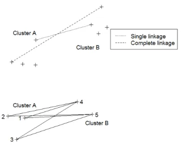
The single, complete, average linkage is illustrated by Figure 1.2:

Figure 1.2: Examples of three inter-cluster distance measures: single, complete and average

1. Single linkage (Sneath, 1957): minimum distance between pair of objects, one in one cluster and one in the other.

2. Complete linkage (Sorensen, 1948): maximum distance between pair of objects, one in one cluster, one in the other.

3. Average linkage (Sokal and Michener, 1958): average distance between pair of objects, one in one cluster, one in the other.

(30)

The kth Nearest Neighbour clustering procedure was proposed by Wong and Lane (1983), and it is designed to be strongly set-consistent based on density estimates. The earlier literature with discussion of density estimating in clustering procedures can be found in Bock (1979), Wishart (1969) and Ling (1972).

Let the observations x1, . . . xn be independent, Wong and Lane (1983) estimate the

density at a pointx byfn(x) given by

fn(x) =k/[nVk(x)],

where Vk(x) is the volume of the smallest sphere centred at x containing k sample

observations. Then the relationship of ‘neighbour’ for two points is given by

Definition 2. Two observations xi and xj are said to be K-neighbours if

d∗(xi, xj)≤dk(xi) ordk(xj),

where d∗ is the Euclidean metric and dk(xi) is the kth nearest-neighbour distance to

point xi.

A distance matrix arises from these density estimates according to the following definition:

Definition 3. The distance d(xi, xj) between the observations xi and xj is

d(xi, xj) = 1 2[ 1 fn(xi) + 1 fn(xj) ] =    n

2k[Vk(xi) +Vk(xj)] if xi and xj are neighbours

∞ otherwise.

Thekth nearest neighbor rule is considered the simplest and most intuitively appeal-ing nonparametric classification procedure (Hall et al., 2008). However application of this method is inhibited by lack of knowledge about its properties, in particular, the parameter selection, and the absence of techniques for empirical choice ofk, and the presence of noisy or irrelevant features. Much effort has been exerted in select-ing or scalselect-ing features to improve classification. Wong and Lane (1983) suggested k= 2log2N to be effective for sample size N from 50 to 500 (see Wong and Schaack, 1982). And its increase should correspond to the increase in sample size. Hall et al.

(31)

(2008) detailed the way in which the value ofk determines the misclassification error, and advised empirical choice ofk to minimize the average error rate. They considered the Possion and Binomial models for training samples, and thekth nearest neighbour method locates the cluster position for each test sample. However, we find these choices are relatively conservative for the sensitivity analysis. In practice, a series of k may be considered, for example, different values of K are used in KNN regression and classification in R package ’caret‘ (from Jed Wing et al., 2013).

1.4.2

Permutation Test

Compared with the abundant discussion about cluster algorithm procedures, little re-search has investigated the properties of significance tests for distinguishing between the hypothesis H0 of a ‘homogeneous’ population and an alternative H1 involving ‘clustering’ or ‘heterogeneity’. But fortunately Lee (1979) and Bock (1985) and most recently Auffermann et al. (2002) contributed to this area. The likelihood ratio (LR) and union-intersection (UI) criteria and a ‘linear discrimination’ statistics are shown in Lee (1979), and these tests are claimed to be equivalent. Meanwhile Bock (1985) considered four types of test statistics: the largest gap between observations, their mean distance (or similarity), the minimum with-in cluster sum of squares resulting from a k-mean algorithm and the resulting maximum F statistics. These tests are used to investigate the uniformity and unimodality hypothesis and alternatives. Al-though Bock (1985) provided theoretical discussion of the test measure, and a possible threshold is suggested with the measurement statistics distribution (asymptotically) estimated, the accuracy for the critical threshold and the power of the test still need to reconsidered. With the development of computing technology, the bootstrap algo-rithm (Efron and Tibshirani, 1993) was applied in testing fMRI data by Auffermann et al. (2002), where Fisher’s linear discriminant function (Fisher, 1936) is chosen as the statistical measure.

Permutation Test and Bootstrap Test:

When we consider the two samples/clusters problem, Fisher’s permutation test (Fisher, 1971) is popularly used. Our target is to test the null hypothesisH0 of no difference between two groupsX1 and X2,

(32)

The equality here meansX1andX2assign equal probabilities to all sets,P rob_X₁{A}=

P rob_X

2{A}for any subsetAof the common sample space of thex1andx2. Normally the test statistic can be the mean difference, ˆd =|X¯1−X¯2|(for scalar variables), and we expect that if theH0 is not true, the value of ˆd will be larger than if H0 is true. To carry out the test, the achieved significance level(ASL) of the test is defined as the probability of observing at least that large a value ˆd∗ when the null hypothesis is true,

ASL=P robH0{dˆ

∗ _≥ _ˆ

d}.

The smaller the value of ASL, the stronger the evidence against H0. Fisher’s per-mutation test is a clever way of calculating an ASL for the general null hypothesis

X1 =X2. First of all, we combine the two groups together as X = (X1,X2), with sample size N =n1+n2. We re-write the data frame as D = (X,R), where vector

R indicates which group each observation belongs to. It consists of n1 individuals from group 1 and n2 individuals from group 2, there are _nN

1

possible R vectors, corresponding to all possible ways of partitioningN elements into two subsets of size n1 and n2. Permutation theory thus considers the permutations of x1’s and x2’s as equally likely ifH0 is true. In other words, let ˆd=S(R,X) for some functionS, and for any one of the _nN

1

possible vectors R∗, the corresponding test statistics ˆ

d∗ = ˆd(R∗) = S(R∗,X)

should be the same as ˆd under H0. The distribution that puts probability 1/ _nN₁

on each one of these ( ˆd∗) is called the permutation distribution of ˆd. The permutation ASL is defined to be the permutation probability that ˆd∗ exceeds ˆd,

ASLperm = P robperm{dˆ∗ ≥dˆ}

= #{dˆ∗ ≥dˆ}/

N

n1

where #{.} denotes the cardinality of the set.

Bootstrap method can be applied to calculate the ASL, which can be done by

[

ASLperm= #{dˆ∗(b)≥dˆ}/B

(33)

More generally, two quantities of carrying out a bootstrap hypothesis test are:

1. A test statistic t(x).

2. A null distribution ˆF0 for the data under H0.

The empirical distribution ˆF0 is a nonparametric estimate specified by the null hy-pothesis H0 given X.

Given these, we generate B bootstrap values of t(x∗) under ˆF0 and estimate the achieved significance level by

[

ASLboot = #{t(x∗b)≥t(x)}/B

Bootstrap tests are useful in situations where the alternative hypothesis in not-well specified, and normally it requires a large B. The choice of test statistic t(x) will determine the power of the test, that is , the chance that we rejectH0 when it is false. Permutation algorithm is quite similar to bootstrap algorithm, and the main difference is that permutation sampling is carried out without replacement while bootstrap with replacement. And their efficiencies are about the same.

1.5

Structure of the Thesis

This thesis mainly focuses on the missing data problem with the model uncertainty issue, and the procedure of missingness can be separated into ignorable and non-ignorable assumptions. Local bias analysis is conducted using an ML method to assess the impact on the estimation of parameters of interest. We recognize that the statistical modelling assumption with parametric models is questioned as the lack of identifiablility or the lack of randomization, thus sensitivity analysis is applied to these problems.

The structure of the thesis is as follows. We first use incomplete data bias analysis to address the model uncertainty problems. In Chapter 2, we will discuss the covari-ate distribution misspecification for partially missing confounder problems. And in Chapter 3, the covariate distribution misspecification and missing data mechanism

(34)

misspecification are both investigated. We use some examples to illustrate the uncer-tainty issue and the local bias analysis. In Chapter 4, we concentrate on measuring the uncertainty sources and propose a novel Monte Carlo sensitivity analysis method to make bias model selection (MC-BMS). Under ignorable missingness, the uncertainty about covariates distribution will be the primary concern. And in Chapter 5, we further apply the incomplete data bias analysis to non-ignorable missing data. And the missing data mechanism bias is calculated given covariate distribution, although it may be difficult to specify in practice. Further discussion based on the MC-BMS method for covariate density specification (based on pattern mixture model frame) will be given in Chapter 5 and discussion for missing data mechanism modelling (based on selection model frame) will be given in Chapter 6. We also discuss the other missing data problem for meta-analysis in Chapter 7, such as publication bias and missing confounder problems. And a robust confidence interval is proposed for meta regression models. Chapter 8 contains conclusions and suggestions for future work.

(35)

Local Sensitivity Analysis for

Missing Covariates Problems

2.1

Introduction

Copas and Eguchi (2005) discussed the model uncertainty issue with missing data by local bias analysis. They used a parametric model for inference when the data generating distribution is close to but not necessarily part of the considered parametric model. Bias is caused by the misspecified working model under incomplete data Y, and the bias is called incomplete data bias by Copas and Eguchi (2005). Lin et al. (2012) noticed that the actual working model may be a conditional model rather than the marginal model under incomplete data, and the so-called marginal model bias is measured under an identifiable local analysis assumption. We follow up their work and extend to partially missing data under ignorable assumption. The bias analysis is a useful tool for identifying the uncertainty parameters (termed asbias parameters) and analysing the model misspecifications, and we will apply it to missing data mechanism misspecification in Chapter 3 and non-ignorable missing data in Chapter 5.

We will introduce Copas and Eguchi’s discussion about uncertainty analysis for miss-ing data problems in Section 2.2, and interpret the incomplete data bias via bias parameters. One example about missing confounder problem will be discussed in Section 2.2.1. We further extend the inference to partially missing confounder prob-lems, and argue that the model uncertainty issue is also important in this case due

(36)

to the lack of identifiablility or the lack of randomization. The incomplete data bias analysis will be performed for a linear regression model under missing completely at random in Section 2.3 and missing at random assumption in Section 2.4. Then we will discuss the ‘double misspecified’ problems for generalized linear models in Section 2.5.

2.1.1

Missing Data Problem

Incomplete data is very common in epidemiology trials, and an example which illus-trate some of the missing data problems is the case control studies to assess the link between alcohol consumption and breast cancer. A linear regression model may be assumed to examine the effect of alcohol use (denoted as variable X) towards breast cancer case (the log odds ratio is taken as the response variableT). Longnecker et al. (1988) reported significant association between the consumption of alcohol and the risk of breast cancer based on a meta-analysis of 16 published epidemiological studies. As agreed by these and later researchers, the estimation of parameter (denoted asθx)

should be adjusted for the potential confounders (e.g. age, see Garland et al., 1999), which is denoted asC. The regression model is given as

t =θ0+θxx+θcc+e (2.1)

where (θ0, θx, θc) are regression coefficients and e∼N(0, σ2) bringst variation.

In practice, the confounder C is not always observed unfortunately and this analysis is likely to be influenced by missing the values and may lead to potential bias. This dissertation analyses the incomplete data biases for the missing data problems and also try to interpret the bias sources via bias parameters. The models we used for bias analysis is then namedbias models.

2.2

Model Uncertainty and Incomplete-Data Bias

A statistical model is merely a parameterized family of probability distributions to which we believe the true distribution belongs (Amari, 1985). Given collected data, we specify a model{f(., θ), θ∈Θ} for inference about parameterθ, which is usually a vector and our interest may be part of it. We conceptually assume the observed

(37)

data is from the true distribution, however in practice, data generating distribution, denoted as g, is not always equal to f. Also we should consider the influence of missing data.

Copas and Eguchi (2005) discussed the model uncertainty issue and incomplete-data bias analysis. They suggested a rather general asymptotic setting for exploring the link between local model uncertainty, defined in an appropriate way. For complete dataZ and incomplete dataY, parametric modelsgZ andgY specify the distribution

ofz andyrespectively. In many cases, inference is based on a working modelfZ while z is in fact generated by a nearby distribution gZ . Following Copas and Eguchi’s

discussion, to formulate distribution in a local neighbourhood of fZ, let uZ(z;θ) be

any scalar function ofz and parameter θ, standardized to have mean 0 and variance 1 under the modelfZ. Then for small values of , the sampling model

gZ =gZ(z;θ, , uZ) = fZ(z;θ) exp{uZ(z;θ)} (2.2)

is non-negative and integrates to 1 up to and including first-order terms in , and so identifies a distribution in the neighbourhood of fZ. If = 0 then gZ = fZ

meaning the working model is the correct model. Intuitively, can be thought of as the ‘magnitude’ of misspecification and uZ can be thought of as the ‘direction’ of

misspecification. If we fix and imagine θ and uZ ranging over all possibilities, gZ

will cover all distribution within a ‘tubular neighbourhood’ of ‘radius’ around the working modefZ. And the distribution of y=y(z) that is induced by gZ is

gY = gY(y;θ, , uZ) = Z (y) fZ(z;θ) exp{uZ(z;θ)}dz ≈ fY(y;θ) exp{uY(y;θ)}, (2.3)

where uY(y;θ) = Ef{uZ(z;θ)|y} and fY is the corresponding working model of fZ

for incomplete data: fY =

R

(y)fZdz. The notation (y) on the intergration sign is interpreted in Section 1.1. These and later approximations are correct to first-order in terms of. We put these inferences into the following lemma:

Lemma 2.1. The data sampling distribution under complete data(Z)isgZ (Equation

2.2), which has the corresponding ‘working model’ fZ. Correspondingly, the

(38)

‘working model’ fY. The estimation of parameters is

θgZ =argθ[Eg{sZ(z;θ)}= 0]≈θ+IZ−1Ef{uZ(z;θ)sZ(z;θ)},

which is the limit of MLE when we use working model fZ but the sampling model is gZ. The estimation from Y is

θgY =argθ[Eg{sY(y;θ)}= 0]≈θ+I_Y−1Ef{uY(y;θ)sY(y;θ)}.

Under the identifiability condition (see Lin et al., 2012), the incomplete-data bias bθ

is defined as the first-order approximation to the difference θgY −θgZ, which is given

by

θgY −θgZ ≈bθ =Ef[uZ(z;θ){IY−1sY(y;θ)−IZ−1sZ(z;θ)}] (2.4)

with IY, IZ, sY, sZ as information matrices and score vectors of fY, fZ respectively.

Detailed proof for Lemma 2.1 is given in Appendix 2.7.1. Lemma 2.1 uses the first order approximation to estimate the bias, and thus require a local analysis assumption to make inference validly, which means that the misspecification quantity is small so thatfZ is in local neighbour ofgZ.

Notice that Copas and Eguchi’s definition of incomplete data bias is given as (θgY −θgZ), which is the difference of estimators from incomplete data distribution gY and complete data distribution gZ. In most literatures, the bias is commonly

defined as the difference between the estimator and true value, that is (θgY −θtrue).

Copas and Eguchi (2005) (page 470) argued that the difference of (θgZ −θtrue) is

the difference of ‘object of interest’ θIN T and ‘object of inference’ θIN F. This is a fundamental problem on how to interpretθ. For example, if θIN T is the mean of the population from which we are sampling, and object of inference θIN F is the value of θ for which the model (noted as gZ) is closest to the true distribution in the

sense of Kullback-Leibler divergence. Royall and Tsou (2003) found θIN F ₌ _θIN T

for the model N(θ, σ2_{) or Possion (}_θ_{) when the model fails, but not for log-normal} distribution. They also argued that parametric inference aboutθ is meaningful only when θIN F ₌_θIN T_{. Our discussion is based on this assumption, then the difference}

(39)

2.2.1

Linear Model with Missing Confounder

Assume we have an experiment design which contains response variableT, and inde-pendent covariatesXandC. VariableXusually describes the treatments or therapies in clinical research. AndC represents the confounder. We denoteZ = (T, X, C) and

Y = (T, X) as the complete and incomplete data respectively, with confounder C missing for all observations. We suppose c ∼ N(0, σ2

c) here but the results can be

extended to other distributions.

Complete data Z = (T, X, C) follows the distribution:

gZ =fT|XC(t, x, c)fXC(x, c).

IfX and C are assumed independent, the working model underZ is

fZ =fT|XC(t, x, c)fX(x)fC(c).

According to equation (2.3), incomplete data Y = (T, X) has distribution:

gY =fY exp(uY)

wherefY is the working model under Y

fY =fT|X(t, x)fX(x)

which is actually the marginal model offZ for the linear regression model if residuals

are normally distributed, see the detailed discussion in Appendix 2.7.3. But if resid-uals are not normally distributed, the ‘double misspecification’ may be considered, see Lin et al. (2012). This case usually happens in non-linear models or generalized linear models, and we will discuss this issue in Section 2.5.

Assume that the response variable has a linear regression model:

t|(x, c)∼N(θ0+θxx+θcc, σ2) (2.5)

(40)

response distribution is an ordinary regression model without c

t|x∼N(θ0+θxx, σt2|x). (2.6)

whereσ2_t_|_xis the variance oftgivenx. Residuals are assumed to be i.i.d with covariates and it can be proved that σ_t2_|_x = σ2 +θ_c2σ_c2. Since x is a scalar variable, there is a bound to limit the quantity of incomplete data bias (Copas and Eguchi, 2005):

Lemma 2.2. Incomplete Data Bias for Linear Model:

The bias of parameter estimation bθx (θx-component) for linear model between

com-plete data model and incomcom-plete data model is bounded by

b2

θx

nvarf(ˆθx)

≤corr(t, c|x)2corr(x, c)2 (2.7)

where n is the sample size.

The first term on the right-hand side of inequality (2.7) is proportional to the partial correlation between t and c given x, which measures how much we lose since not observing the hidden variable c. The second term is the dependence between the treatments (X) and confounder (C) that is caused by the lack of randomization, which is a measure of non-ignorability in the design. The most troublesome confounder is one which is linearly correlated with treatment, see more discussion in Appendix 2.7.2.

Corollary 2.1. When corr(x, c) = 0 and under the ignorable assumption we have

bθx = 0.

Below we will extend the uncertainty problems for partially missing confounder data problems.

2.3

Partially Missing Confounder under MCAR

2.3.1

Bias Models

In this section, we continue to discuss the missing data problem in (2.1). Now con-founder C is partially missing with probability π, and suppose its missing type is

(41)

missing completely at random, which indicates π is a constant. We denoteR as an indicator vector:

r=    1, c observed; 0, cmissing. (2.8)

The complete data set isZ = (T, X, C, R), withRBernoulli distributedR ∼B(1, π). And the corresponding incomplete data set isY = (T, X, C(r)_{, R}_{), where}

c(r)=    c, r = 1; R, r = 0. (2.9)

The symbol_R used here means whenr= 0 all we know is that ctakes some value in R= (−∞,∞).

Starting from the sampling model, we rewrite the density function gZ as follows:

gZ(z;θ, π) = fZexp{uz}

= fT|XC(t|x, c;θ)fXC(x, c)h(r;π)

where the missing data mechanism component is h(r;π) = πr₍₁₋_π₎1−r_{. And the}

working model (assumingX and C are independent) is given as :

fZ =fT|XC(t|x, c;θ)fX(x)fC(c)h(r;π). (2.10)

Then the misspecification of the model is caused by the association between observed variableX and missing variable C, represented by

exp{uz}=

fXC(x, c)

fX(x)fC(c)

. (2.11)

As the misspecification is related to [XC] only1_{, we write}_u

Z asuXC in the following.

AndbXC represents the incomplete data biasbθ caused by covariate density

misspec-ification. Here the incomplete data bias can also be termed covariate bias according to the bias source.

(42)

As covariateC is partially missing, we split all casesY into two parts: complete cases and incomplete cases, Y = (Ycc,Yic). For complete cases (when r= 1)

fYcc =fZ =fT|XC(t|x, c)fX(x)fC(c)h(r= 1;π).

While for incomplete cases (whenr = 0)

fYic = Z (y) fZdz = Z (y) f(t, x, c)h(r = 0;π)dz = Z c fT|XC(t|x, c)fX(x)fC(c)h(r = 0;π)dc = fX(x)h(r= 0;π) Z c fT|XC(t|x, c)fC(c)dc = fT|X(t|x)fX(x)h(r = 0;π), wherefT|X(t|x) = R

cfT|XC(t|x, c)fC(c)dc. Similarly to the discussion given in Section

2.2.1, the working model under incomplete data isfY =

R

(y)fZdz, the marginal model of complete data working model.

Then we write the models into one general form:

Estimation of parametersθ fromfY is calculated by maximizing the log-likelihood of

(2.12), which is biased if covariate correlation is not equal to zero. The incomplete data bias analysis is conducted below.

(43)

2.3.2

Incomplete Data Bias

For complete dataZ = (T, X, C, R), we use a linear fixed effect model to fit the data

t|(x, c)∼N(θ0+θTxx+θcc, σ2) (2.15)

where σ2 _{is the variance of error and variable} _x _{can be a vector. And with the} incomplete data :

t|(x, c, r)∼N(θ0+θxTx+rθcc, σ2+ (1−r)θ2cσ

2

c).

For complete cases, the incomplete data model is the same with the complete data model; while for incomplete cases, we assume (t|x, r = 0) ∼ N(θ0 +θTxx, σ2+θ2cσc2)

which is similar to the totally missing confounder problem discussed in Section 2.2.1. Here we use the ML method to estimate the parameters θ = (θ0, θxT, θc) and the

incomplete-data bias. For complete data and incomplete data, the log-likelihood for the linear model is

lZ(θ;z) = logf(t|x, c;θ) = Cons−logh(r)−1 2log(σ 2 )− 1 2 (t−θ0−θTxx−θcc)2 σ2 lY(θ;y) = logf(t|x, c, r;θ) = Cons−logh(r)−1 2log(σ 2_{+ (1}₋_r₎_θ2 cσ 2 c)− 1 2 (t−θ0−θxTx−rθcc)2 σ2_{+ (1}₋_r₎_θ2 cσ2c .

The above formulas have component −logh(r) which is constant under MCAR and thus can be ignored. Here, we assumeσ2 _{is given (it can be replaced by its estimation} s2 _{which can be obtained from each study). From log-likelihood} _l

Z and lY, the score

functions under complete data and incomplete data are

sZ(z;θ) =      t−θ0−θxTx−θcc σ2 (t−θ0−θTxx−θcc)x σ2 (t−θ0−θxTx−θcc)c σ2      andsY(y;θ) =      t−θ0−θTxx−rθcc σ2₊₍₁₋_r₎_θ2 cσ2c (t−θ0−θTxx−rθcc)x σ2₊₍₁₋_r₎_θ2 cσ2c (t−θ0−θTxx−rθcc)rc σ2₊₍₁₋_r₎_θ2_σ2     

(44)

respectively. Fisher information matrix for complete data is IZ = 1 σ2      1 µx µc µx Σx E(xc) µc E(xc) Σc      , (2.16) whereµx =E(x), µc =E(c),Σx =E(xxT), Σc=E(c2). Similarly, IY = π σ2      1 E(x|r= 1) E(c|r= 1) E(x|r= 1) E(xxT|r= 1) E(xc|r= 1) E(c|r = 1) E(xc|r= 1) E(c2_|_r _{= 1)}      +1−π σ2 Y      1 E(x|r= 0) 0 E(x|r= 0) E(xxT_|_r_{= 0) 0} 0 0 0      (2.17) whereσ2

Y =σ2+θc2σc2. Using Lemma 2.1, we have the incomplete data bias as

θgY −θgZ =Ef[uZ(z;θ){IY−1sY(y;θ)−IZ−1sZ(z;θ)}].

In this chapter, we only concentrate on the covaraite distribution misspecification, and the incomplete data bias is mainly generated by the correlation betweenX and C, so we call itcovariate biasparticularly, denoted bybXC. For simplifying notations,

we definev = (1, x, rc)T_,_v

1 = (1, x, c)T andv0 = (1, x,0)T. Since ET|XC(sZ) = 0 for

allx and c, thus

bXC = IY−1EfZ{uXCsY} −IZ −1_E fZ{uXCsZ} = IY−1[πE{uXCsY|r=1}+ (1−π)E{uXCsY|r=0}] −IZ−1EXC{uXCET|XC(sZ)} ≈ IY−1(1−π)E[uXC cθc σ2 Y v0] = θc(1−π) IY−1 σY E(cuXCv0).

In this chapter we consider the uncertainty caused by missing covariate and thus the misspecification of f(x, c). As shown in formula (2.11), if the misspecification

(45)

quantity is small, then EfZ(cuXCv0) = EfZ{cv0log f(x, c) f(x)f(c)} ≈ EX,C{cv0 f(x, c)−f(x)f(c) f(x)f(c) } = EXC(cv0)−EX,C(cv0) = (0,cov(x, c),0)T.

Here EXC indicates the expectation under distribution f(x, c), while EX,C indicates

the expectation under independent distributionf(x)f(c). So we have the incomplete data bias for θgY as

bXC = θc(1−π)IY−1 σ2 Y      0 cov(x, c) 0      . (2.18)

If covariate correlation corr(x, c) = 0, the incomplete data biasbXC =0 as we stated

in Corollary 2.1. If we write the inverse of the Fisher information matrixIY as

IY−1 =      Iθ0θ0 _Iθ0θx _Iθ0θc Iθ0θx _Iθxθx _Iθxθc Iθ0θc _Iθxθc _Iθcθc      ,

then we have the incomplete data bias for θx-component:

bθx ≈θc(1−π)

Iθxθx

σ2

Y

cov(x, c). (2.19)

If covariateC is totally missing (π = 0), then Iθxθx ₌ σ 2 Y σ2 xand bθx =θc Iθxθx σ2 Y

cov(x, c) = (Iθxθx₎1/2_corr(_{t, c}_|_x_)corr(_{x, c}₎ _(2.20)

since corr2(t, c|x)≈ θ 2 cσc2 σ2 Y

(46)

that the incomplete data bias for partially missing data is also impacted by the covari-ate correlation, but the size of the bias gets smaller than totally missing confounder problem as (1−π)<1.

2.4

Partially Missing Confounder under MAR

Another missing data mechanism is termed as missing at random (MAR, Rubin, 1976). It means that the probability that a variable is observed/missing