Title
longitudinal data analysis
Author(s)
Zheng, XY; Fung, WK; Zhu, ZY
Citation
Statistica Sinica, 2014, v. 24 n. 2, p. 515-531
Issued Date
2014
URL
http://hdl.handle.net/10722/199235
VARIABLE SELECTION IN ROBUST JOINT MEAN AND COVARIANCE MODEL FOR LONGITUDINAL
DATA ANALYSIS
Xueying Zheng1, Wing Kam Fung2 and Zhongyi Zhu1 1Fudan University and 2The University of Hong Kong
Abstract: In longitudinal data analysis, a correct specification of the within-subject covariance matrix cultivates an efficient estimation for mean regression coefficients. In this article, we consider robust variable selection method in a joint mean and covariance model. We propose a set of penalized robust generalized estimating equations to simultaneously estimate the mean regression coefficients, the general-ized autoregressive coefficients, and innovation variances introduced by the modified Cholesky decomposition. The set of estimating equations select important covari-ate variables in both mean and covariance models together with the estimating procedure. Under some regularity conditions, we develop the oracle property of the proposed robust variable selection method. Finally, a simulation study and a detailed data analysis are carried out to assess and illustrate the small sample per-formance; they show that the proposed method performs favorably by combining the robustifying and penalized estimating techniques together in the joint mean and covariance model.
Key words and phrases: Covariance matrix, penalized generalized estimating equa-tion, longitudinal data, modified cholesky decomposiequa-tion, robustness, variable se-lection.
1. Introduction
Longitudinal data arise more and more frequently in a variety of scientific domains that seek insightful and comprehensive research in a branch of statisti-cal modeling. Different from other types of data, we often assume independence among distinct subjects but dependence within each subject; within-subject cor-relation raises a fundamental challenge for the analysis of longitudinal data. Liang and Zeger (1986), a milestone in the development of methodology for longitudinal data analysis, proposed generalized estimating equations (GEE) for estimation of generalized linear regression coefficients. The main advantage of their method is that even when the within-subject correlation is treated as a nuisance parameter with an assumed parsimonious structure, GEE still brings about a consistent estimator for the mean regression model. Subsequential, Qu, Lindsay, and Li (2000) used the quadratic inference function (QIF) to enhance
the efficiency by considering the structure of the covariance matrix. Taking ro-bustification into account, He, Fung, and Zhu (2005) proposed the robust GEE method to prevent the unexpected influence from outliers in a longitudinal data set.
Ignoring the within-subject correlation can result in an inefficient estimator of a regression model. In practice, the within-subject covariance structure itself may be of scientific interest. Relevant topics here include component analysis and factor analysis in multivariate statistical problems. Recent research on the estimation of the covariance matrix includes, but is not limited to, Rothman, Levina, and Zhu (2009), El Karoui (2008) and Bickel and Levina (2008).
Similar to the mean regression, covariances may be dependent on various explanatory variables. Pourahmadi (1999, 2000) proposed a joint mean and covariance regression model by decomposing the covariance matrix employing generalized autoregressive coefficients and innovation variances. Ye and Pan (2006) extended the joint model under the framework of generalized estimating equations which required no assumptions on the distribution of the data. By introducing generalized autoregressive coefficients and innovation variances, their joint model eliminated the positive definiteness constraint in estimation of the covariance matrix. Instead, three generalized estimating equations were proposed to estimate the covariance matrix and the mean simultaneously.
A number of developments have been followed, see Fan, Huang, and Li (2007), Fan and Wu (2008), and Xu and Mackenzie (2012). Leng, Zhang, and Pan (2010) generalized Ye and Pan’s model to a semiparametric joint mean and covariance model. Mao, Fung, and Zhu (2011) extended Leng, Zhang, and Pan (2010)’s work further to a generalized partially linear varying coefficient model. Zheng, Fung, and Zhu (2013) extended the robust estimating equation in He, Fung, and Zhu (2005) to the joint mean and covariance model by creating three robust estimating equations to mitigate the effect of outliers in both mean and covariance estimation.
Variable selection is a technique for selecting a subset of relevant covari-ates in constructing reliable statistical models. Many variable selection methods are based on the penalized likelihood or penalized estimating equations. Com-monly used penalties include LASSO, ALASSO (adaptive lasso in Zou (2006)) SCAD, and Hard penalties. In longitudinal data analysis, Fu (2003) proposed the penalized generalized estimating equation with LASSO penalty. Other vari-able selection criteria include AIC andCp, extended by Pan (2001) and Cantoni, Flemming, and Ronchetti (2005), respectively, to the case of longitudinal data under the framework of GEE.
In contrast, little work has been done on covariance variable selection or identification. Jeng and Daye (2011) noticed that to curve the sparsity in the
covariance matrix can improve the efficiency on mean estimation, especially in high dimensional problems, though their main objective was still the mean esti-mation. Within the framework of the joint mean and covariance model, Huang et al. (2006) proposed covariance selection and estimation via penalized nor-mal likelihood. Kou and Pan (2011) proposed a penalized maximum likelihood method for the joint model that employed variable selection in both models si-multaneously, the covariance matrix being treated as of equal importance as the mean.
In this paper, we develop a penalized robust estimating equations based method to select important explanatory variables. Simulation studies have shown that both the classical GEE and the joint mean and covariance model are sensi-tive to outliers, see details in He, Fung, and Zhu (2005) and Zheng, Fung, and Zhu (2013). Nevertheless, the discussion on robust variable selection methods has been limited. We consider the SCAD and ALASSO penalties, and show the oracle property of the proposed robust variable selection method. In data analysis, the robust variable selection procedure can provide standard errors for mean coefficients estimation, due to sensible covariance matrix modeling and the accommodation of outliers in both subject and observation levels.
The remainder of this article is organized as follows. Section 2 describes the main model and its asymptotic properties. Simulation results are given in Section 3. In Section 4, we apply the proposed method to a hormone data set.
2. Robust Variable Selection in Joint Mean and Covariance Model 2.1. Joint mean and covariance model
Suppose that we have a sample of m subjects. Let yi = (yi1, . . . , yini) T be theni repeated observations at time pointti = (ti1, . . . , tini)
T of theith subject. Let E(yi) = µi = (µi1, . . . , µini)
T and Cov(y
i) = Σi be the ni ×1 mean vector and ni×ni covariance matrix ofyi, respectively.
To eliminate the constraint of positive definiteness in estimation of the covari-ance matrix Σi, we implement a modified Cholesky decomposition by introducing a unique lower triangular matrix Φi with 1’s as diagonal entries and a unique diagonal matrix Di with positive diagonals such that
ΦiΣiΦTi =Di.
Here the lower-diagonal entries of Φi are the negatives of the autoregressive coefficients ϕijk defined in
ˆ yij =µij + j−1 ∑ k=1 ϕijk(yik−µik),
the linear least squares predictor ofyij based on its predecessorsyi(j−1), . . . , yi1.
The diagonal entriesσ2
ij ofDi are the innovation variancesσij2 =var(εij), where εij =yij −yijˆ .
We adopt linear models for the mean, generalized autoregressive parameters, and innovation variances as in Ye and Pan (2006):
µij =xTijβ, ϕijk =gijkT γ, logσ2ij =zijTλ, (2.1) where xij, gijk, and zij are p×1, q ×1 and d×1 vectors of covariates, and β, γ and λ are associated parameters. The covariates gijk and zij may contain baseline covariates, time and associated interactions. The log-linear model of the innovation variance follows Cook and Weisberg’s (1983) model for the variance. Cook and Weisberg developed a log-linear model that allows for dependence of the variance on an arbitrary set of variables. In practice, the whole set of the covariates is difficult to define. An orthogonal form for a polynomial of time was recommended as the covariate for the autoregressive component by Ye and Pan (2006):
gijk = (1, (tij−tik), (tij−tik)2, . . . , (tij −tik)q−1)T.
The linear assumption in (2.1) can be replaced by quadratic assumptions, or the use of nonparametric or semiparametric models after the decomposition, see Mao, Fung, and Zhu (2011) and Leng, Zhang, and Pan (2010). To simplify matters we start from the linear assumption.
In the models at (2.1), estimation for generalized autoregressive coefficients and innovation variances are treated as important as the estimation for the mean. Letθ = (θ1, . . . , θs)T = (β1, . . . , βp;γ1, . . . , γq;λ1, . . . , λd)T, where s=p+q+d. To select important subsets of the covariates, we assume that all interesting explanatory variables, together with their interactions, are involved. By using the same λ, the proposed method is applicable for correlated data as long as the correlated (or longitudinal) measurements have similar correlation structure between clusters.
2.2. Penalized robust generalized estimating equations
We propose a penalized robustified generalized estimating equations
U(θ) = ([U1(β)]T, [U2(γ)]T, [U3(λ)]T)T,
for the mean, generalized autoregressive parameters, and innovation variances, respectively: U1(β) = m ∑ i=1 XiT(Viβ)−1hiβ(µi(β))−mqτ(1)(|β|)sgn(β) = 0, (2.2)
U2(γ) = m ∑ i=1 TiT(Viγ)−1hγi(ˆri(γ))−mqτ(2)(|γ|)sgn(γ) = 0, (2.3) U3(λ) = m ∑ i=1 ZiTDi(Viλ)−1hλi(σi2(λ))−mqτ(3)(|λ|)sgn(λ) = 0, (2.4) where hβi(µi(β)) = Wiβ[ψβ(µi(β))−Ciβ(µi(β))], hγi(ˆri(γ)) = Wiγ[ψγ(ˆri(γ))− Ciγ(ˆri(γ))] and hλi(σi2(λ)) = Wiλ[ψλ(σ2i(λ))−Ciλ(σi2(λ))] act as the core of the estimating equations with Xi = (xTi1, . . . , xTini)
T, Z
i = (ziT1, . . . , zinTi) T, g
ij = (gijT1, . . . , gTij(j−1))T and Ti = (gTi1, . . . , ginTi)T.
Equations (2.3) and (2.4) are in agreement with (2.2), in which ri in U2(γ)
and ε2i in U3(λ) play roles similar to that of yi in U1(β), and can be viewed as
working responses. Here covariance estimation is treated the same mean esti-mation in the proposed model, in the spirit of the joint model in Ye and Pan (2006).
We specify items in (2.2)−(2.4). InU2(γ), ri and ˆri areni×1 vectors with
jth components rij =yij −µij and ˆrij =E(rij|ri1, . . . , ri(j−1)) = ∑j−1
k=1ϕijkrik,
where ∑0k=1 is zero when j = 1. In U3(λ), εij = yij −yˆij and ε2i and σi2 are ni×1 vectors with jth components ε2ij and σij2, respectively, where in fact E(ε2i) = σi2. Moreover, TiT =∂ˆrTi /∂γ is the q×ni matrix with the jth column ∂ˆrij/∂γ =
∑j−1
k=1rikgijk and Di= diag{σ 2
i1, . . . , σin2i}.
Again at (2.2)−(2.4), Viβ = Ai−1/2Σi, Ai is the diagonal elements of Σi, Viγ =Di1/2,Viλ=Ae−i 1/2Σi, ande Aie is the diagonal elements ofΣi. The sandwiche working covariance structureΣie =Bi1/2Ri(δ)Bi1/2 can be used to model the true
e
Σi = Cov(ε2i) with Bi = 2diag{σ4i1, . . . , σ4ini} and Ri(δ) mimics the correlation betweenε2ij and ε2ik by introducing a new parameter δ. This idea was proposed by Ye and Pan (2006).
The parameter δ has little effect on the estimation in practice. Consider-ing the AR(1) structure, we can estimate δ by the slope from the regression of log(ˆε2ij,εˆ2ik) on log(|tj −tk|). Details can be found in Example 4 in Liang and Zeger (1986). In our simulations and data analyses, the estimate of δ always falls in the interval [0,0.3]. Moreover, results in Table 3 for simulation Study 2 also imply that we can ignore the difference between the independent and AR(1) structure forRi(δ).
Penalized robust generalized estimating equations are distinguished from conventional generalized estimating equations in two aspects. First, the un-desirable influence of outliers is controlled. In the core of the estimating equa-tions, ψβ(µi) = ψ(A−i 1/2(yi −µi)), ψγ(ˆri) = ψ(Di−1/2(ri −ri)), andˆ ψλ(σi2) = ψ(Ae−i 1/2(ε2i −σi2)). The function ψ(·) is chosen to limit the influence of out-liers in the response variable, and a common choice is Huber’s score function
ψc(x) = min{c,max{−c, x}} for some constant c, c = 2 in our implementa-tion. To ensure Fisher consistency, we use Ciβ(µi) = E[ψ(A−i 1/2(yi −µi))], Ciγ(ˆri) =E[ψ(Di−1/2(ri−ˆri))] and Ciλ(σ2i) =E[ψ(Aei−1/2(ε2i −σ2i))]. When yi’s are normal, the three expectations depend only on the choice of constant c in Huber’s score function. We can also assign weights to each subject by diago-nal weighting matrices Wiβ = diag(wiβ1, . . . , wβin
i), W γ i = diag(w γ i1, . . . , w γ ini) and Wiλ = diag(wλi1, . . . , winλi). Similar to Qin, Zhu, and Fung (2009), the weight functionwij is chosen to be the Mahalanobis distance
wij =w(pij) = min { 1, [ b0 (pij−mp)TS−1 p (pij−mp) ]ρ/2} ,
withρ≥1, wheremp andSp are some robust estimates of the location and scale ofpij such as the minimum covariance determinant estimators. We introduce the weight function to bound the influence of leverage points, covariate space only. As indicated in He, Fung, and Zhu (2005), we can include certain covariates that are likely to contribute to the leverage. In our simulation study, b0 is chosen
as the 95th percentile of the chi-squared distribution with degrees of freedom equal to the dimension ofpij and ρ is fixed as 1. For simplicity and consistency, we choose pij = xij for all three weighting matrices and denote them as Wi = diag(wi1, . . . , wini).
Selecting variables is achieved by adding a penalty term to each estimating equation. Usually, qτ(l)(·) is the first derivative for some penalty pτ(l)(·), where l = 1,2,3. For brevity, we replace pτ(1), pτ(2) and pτ(3) by pτ and qτ(1), qτ(2) and qτ(3) by qτ when no misunderstanding arises. In the simulation and data analyses, we only consider SCAD and ALASSO penalties to show the asymptotic properties. Fan and Li (2001) defined the smoothly clipped absolute deviation (SCAD) penalty function:
pτ(|θ|) =τ(|θ|){I((|θ|)< τ)}+ (a− |θ|/2τ) a−1 I(τ <(|θ|)< a) + a 2τ 2(a−1)(|θ|)I{(|θ|)≥aτ},
in which a = 3.7 was suggested by the authors. As a compromise between LASSO and Hard penalties, SCAD enjoys unbiasedness, sparsity and continuity properties simultaneously.
As a consistent version of theL1penalty, ALASSO penalty ispτ =τ|θ|w, for a known data–driven weightw. In this paper, we employ the weight w= 1/|θ˜|, where ˜θ is the regression coefficient estimate obtained from solving (2.2)−(2.4) without penalty.
2.3. Asymptotic properties
We write the m subjects–based penalized estimator ˆθm= ((ˆθsm1)T, (ˆθms2)T)T for the true value θ0 = ((θs01)T, (θ
s2
0 )T)T, where θ
s1
0 and θ
s2
0 are the nonzero
and zero components of θ0, respectively. Denote the dimension of θs01 by s1 and
s=s1+s2. The parameter space is assumed compact and the true value θ0 is
in the interior of the parameter space Θ.
In what follows we show that the penalized estimator ˆθm exists and con-verges to θ0 at the rate Op(m−1/2), implying that it has the same consistency
rate as the ordinary estimator. We prove that the√m–consistent estimator ˆθs1 m is asymptotically normally distributed and possesses the oracle property under certain regularity conditions.
Theorem 1. Under the assumptions in S1 of the supplementary material,
(a) there exists an approximate zero-crossing solution θˆ of U(θ) = 0, such that
ˆ
θ=θ0+Op(m−1/2);
(b) for any √m consistent approximate zero-crossing solution of U(θ) = 0, we have
lim m→∞P{
ˆ
θj = 0, j > s1}= 1.
The definition of the zero-crossing estimator ˆθ, which is introduced in John-son, Lin, and Zeng (2008), is given in S1 of the supplementary material. Theorem 1 implies that when we choose a properτm, our robust penalized GEE approach can simultaneously achieve √m consistency of the regularized regression coeffi-cient estimation and consistency of variable selection.
To obtain the asymptotic distribution of ˆθ, we take B = limm→∞(1/m) Cov[UR(θ
0)] and assume it to be positive definite. The definition of UR(θ0) is
given in supplement S1. We assume κm(θ) = E[m1UR(θ)], κm(θ0) = 0, κm(θ) is
continuous on Θ, and κm(θ) is differentiable at θ0 with nonsingular derivative
matrix G. Define cm = (qτm(|θ s1 01|)sgn(θ s1 01), . . . , qτm(|θ s1 0s1|)sgn(θ s1 0s1)) T and Ω = diag{−qτ′m(|θ0|)sgn(θ0)},whereτm is equal to eitherτm(1),τm(2), orτm(3), depending on whether θ0j is a component of β0, γ0, or λ0 (1 ≤ j ≤ s). θ0j is the jth component ofθ0, and θ0s1j is the jth component ofθ
s1
0 (1≤j≤s1).
Theorem 2. Under the conditions given in S1 of the supplementary material, for the SCAD penalty we have
√ m(Gs1 m + Ωsm1){θˆsm1 −θ s1 0 + (Gsm1 + Ωms1)−1cm} →Ns1(0, B s1) in distribution, where Bs1,Gs1
m, and Ωsm1 are the s1×s1 submatrix ofB,G, and
Ω corresponding to the nonzero componentsθs1 0 .
As a result, the asymptotic covariance matrix Cov(ˆθs1 m) of ˆθsm1 is 1 m(G s1 m+ Ωsm1)−1Bˆms1(Gsm1+ Ωsm1)−1.
Thus, our proposed robust penalized joint model based on the SCAD penalty possesses the oracle property. Proofs of Theorems are sketched in S1 of the supplementary material.
2.4. Implementation
An iterative MM algorithm for estimating β,γ and λ is described in detail in S2 of the supplementary material. Meanwhile, the choice of τ is critical. In practice, we selectτ(1) by minimizing the robustified generalized cross-validation (GCV) criterion
GCVβ(τ) =
RSSβ(τ)/m
{1−d(τ)/m}2,
whereRSSβ(τ) is the robustified residual sum of squares m
∑
i=1
[Wiψ(A−i1/2(yi−xiβˆτ))]2,
and d(τ) is the effective number of parameters, dβ(τ) = tr([ ˆG(β)+∆τ( ˆβτ)]−1 [ ˆG(β)]T); here ˆβτ is the solution of the penalized robust GEE when τ is fixed. We select ˆτ = argminτGCVβ.
Similar to the choice of τ(1) we select tuning parameters τ(2) and τ(3) by minimizing the robustified GCV statistics
GCVγ(τ) = RSSγ(τ)/m {1−dγ(τ)/m}2 , GCVλ(τ) = RSSλ(τ)/m {1−dλ(τ)/m}2 ,
whereRSSγ(τ) =∑mi=1[Wiψ(Di−1/2(ri−ri))]ˆ 2 andRSSλ(τ) =∑mi=1[Wiψ( ˜A−i 1/2 (ˆε2
i−σˆi2))]2. dγ(τ) anddλ(τ) are the effective numbers of covariance parameters. To avoid computational burden, we recommend selecting parameters sequen-tially, as follows
(1) Fix τ(2) =τ(3)= 0, choose ˆτ(1)= argminτ(1)GCVβ(τ(1));
(2) Fix τ(1) = ˆτ(1) and τ(3) = 0, choose ˆτ(2) = argminτ(2)GCVγ(τ(2)); (3) Fix τ(1) = ˆτ(1) and τ(2) = ˆτ(2), choose ˆτ(3)= argminτ(3)GCVλ(τ(3)); (4) The final choice is (ˆτ(1),ˆτ(2),τˆ(3)).
The process of tuning parameter selection has merits aside from reducing the computational burden. From a numerical point of view, minimizing GCVγ and
GCVλ does not always benefit mean estimation. Sequentially selecting tuning parameters lets us adjust and stabilize selection while balancing the importance of estimation for the mean and the covariance structure.
3. Simulation
We conducted a simulation study to assess the performance of the proposed estimators on three aspects: The efficiency of our robust model compared with the corresponding non-robust version; the necessity of the robust method for the presence of outliers; comparison with the classical GEE method under covariance matrix misspecification.
We compared model errors of different variable selection procedures using median of model error (MME), where model errors are evaluated, following Fan and Li (2001) as
M Eβ = ( ˆβ−β0)TXXT( ˆβ−β0),
M Eγ= (ˆγ−γ0)TT TT(ˆγ−γ0), M Eλ= (ˆλ−λ0)TZZT(ˆλ−λ0),
where X = (X1T, . . . , XmT)T, T = (T1T, . . . , TmT)T, and Z = (Z1T, . . . , ZmT)T. We employ average correctly fit percentage (CF%) to measure the accuracy of the model selection procedure, where correctly fit means that the procedure selects the exact subset model. Moreover, we compare the average numbers of regression coefficients that are correctly shrunk (CS) to zeros. Replications of each scenario were at 200.
We generated balanced data sets, ni = n, for convenience. In practice, our method also works well for the nearly balanced data set (Zhou and Qu (2012)). In the data example, we can also handle unbalanced data when the observation time information is available; this is a reasonable assumption for longitudinal data, as the subjects’ measurements are recorded along with the observation time. Study 1. We simulated 100 (or 200) subjects, each of which had 5 observations that were multivariate normalN5(µi,Σi). The true values of the mean
parame-ter and log-innovation variances were β = (3,0,0,−2,1,0,0,0,0,−4)T and λ= (0,1,0,0,0,−2,0)T, respectively. Two specifications are designed for generalized autoregressive parameters; γ = (0,0,0,0,0,0,0)T and γ = (0.2,0,0,0,0,0,0)T. The mean covariates xij = (xijt)10t=1 were drawn from the multivariate normal
with mean 0 and covariance matrix of AR(1) structure with variance σ2 = 1 and correlation parameter ρ = 0.5 (i = 1, . . . ,100; j = 1, . . . ,5). Then gijk = (xijt −xikt)t7=1 and zij = (xijt)7t=1 were covariates for the generalized
autoregressive parameters and the log-innovation variances. Using these values, the mean µi and covariance matrix Σi were constructed through the modified Cholesky decomposition from (2.2)−(2.4). The responses yi’s were then drawn from N(µi,Σi) (i= 1, . . . ,100).
We consider two contaminations:
C0: randomly choose 1% ofxij1 to bexij1−1;
C1: randomly choose 2% ofxij1 to bexij1−3 and 2% ofyij to beyij+ 10. NC represents no contamination situation hereafter. C1 is a commonly used contamination setting in previous research on robust methods, and we consider a tiny contamination in C0. The initial value of the mean estimation was obtained from the robust GEE estimation in He, Fung, and Zhu (2005) with independent working correlation that guarantees consistency of the autoregressive parameters and innovative parameters after the first iteration. If the covariance matrix falls into the spanned space of the covariates, the proposed method converges quickly under no contamination, usually in a few steps. However, in non-robust modeling, the traditional MM algorithm has a large probability of non-convergence under contaminations. Typically, in C1, 180 of 200 replications cannot obtain a final estimation due to divergence of iteration in covariance estimation, even when the initial value of estimation for the mean parameter β is close to the true value. Moreover, in 10%-20% of replications the non-robust algorithm fails to converge in C0, where the perturbation is almost negligible.
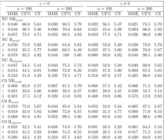
To check asymptotic properties, we simulated with sample size of 100 and 200 subjects. In Table 1, we list the median of model error (MME), average correctly fit percentage (CF%), and average numbers of regression coefficients that are correctly shrunk (CS) for both robust and non-robust methods, under NC (no contamination) and C0 (tiny contamination). Notice that the results for C0 were obtained based on convergence cases only. Rscad and Ralasso represent the proposed robust method employing SCAD and ALASSO, respectively. NR is the non-robust method.
As the number of subjects m increases, the MME of both robust and non-robust methods decreases, while CF% and CS approach 1 and the true number of zero parameters, respectively. These are consistent with the oracle property. The Rscad and NR methods perform equally well in variable selection under NC, although an acceptable loss of efficiency for the robust method can be detected from the slightly larger MME (in NC Rscad compared to NC NR). However, under C0, the robust method apparently outperforms the non-robust method in both estimation efficiency and variable selection. Especially in covariance model identification, the non-robust method fails to correctly identify the innovation variance model under small contamination in most replications.
We compare the performance of Rscadand Ralasso to find that Rscad outper-forms Ralasso inβ and λestimation and Ralasso performs better inγ estimation. In fact, SCAD allows almost no penalty if the true parameter is far from 0 while ALASSO penalizes all parameters, which increases the MME, especially inλ. In
Table 1. Parameter estimation and selection in Study 1.
γ= 0 γ̸= 0
n= 100 n= 200 n= 100 n= 200
MME CF% CS MME CF% CS MME CF% CS MME CF% CS
NC NRscad β 0.040 66.0 5.61 0.030 80.5 5.79 0.032 56.5 5.47 0.021 73.5 5.70 γ 0.016 36.5 5.86 0.000 76.0 6.62 0.021 45.0 5.09 0.004 86.0 5.82 λ 0.057 73.5 4.71 0.032 93.5 4.93 0.043 77.5 4.71 0.026 96.0 4.96 NC Rscad β 0.050 72.0 5.68 0.040 84.0 5.82 0.039 53.0 5.38 0.026 73.0 5.70 γ 0.018 35.5 5.77 0.000 69.5 6.49 0.025 37.5 5.00 0.006 76.0 5.67 λ 0.078 92.5 4.92 0.048 100 5.00 0.060 93.0 4.92 0.040 99.5 5.00 NC Ralasso β 0.047 54.5 5.41 0.033 75.5 5.73 0.049 52.0 5.38 0.030 69.0 5.65 γ 0.012 44.5 6.01 0.000 72.0 6.50 0.021 47.0 5.00 0.003 85.5 5.85 λ 0.242 51.0 4.28 0.193 73.5 4.71 0.318 67.0 4.57 0.265 86.0 4.84 C0 NRscad β 0.068 65.0 5.57 0.067 81.5 5.79 0.068 57.5 5.42 0.066 71.5 5.63 γ 0.021 33.0 5.66 0.000 59.5 6.37 0.061 28.0 4.45 0.039 52.5 5.14 λ 0.331 17.5 3.12 0.520 15.0 3.02 0.408 19.0 3.06 0.575 12.0 2.83 C0 Rscad β 0.053 72.0 5.67 0.043 85.0 5.84 0.052 52.0 5.34 0.065 87.5 5.87 γ 0.018 35.0 5.82 0.000 72.0 6.55 0.040 31.5 4.77 0.000 71.0 6.53 λ 0.068 91.0 4.91 0.052 99.5 5.00 0.088 85.0 4.83 0.069 99.0 4.99 C0 Ralasso β 0.055 52.5 5.41 0.038 74.0 5.70 0.091 50.5 5.29 0.061 64.5 5.54 γ 0.013 41.5 5.93 0.000 74.5 6.55 0.049 28.5 4.54 0.017 71.5 5.61 λ 0.280 43.5 4.22 0.224 67.5 4.63 0.550 60.0 4.49 0.420 84.0 4.82
Simulation results of median of model error (MME), average correctly fit percentage (CF%), and average numbers of regression coefficients that are correctly shrunk (CS) for both robust (Rscad, Ralasso) and non-robust (NR) methods, under NC (no contamination) and C0 (tiny contamination), with 200 replications.
sum, although both robust methods can resist the contamination according to our simulations, Rscad is preferred.
Standard errors for SCAD estimators in Study 1 for non-zero parameters (β1, β4, β5, β10, γ1, λ2, and λ6) are attached in Table S3.1 of the
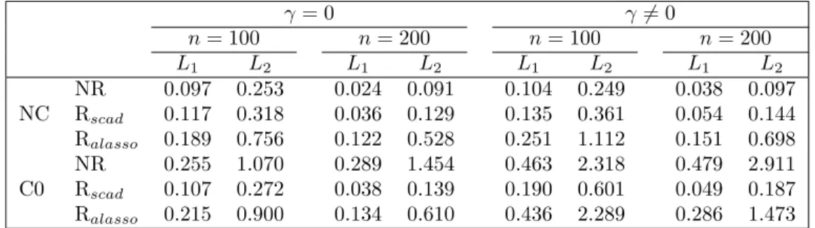
supplemen-tary material. In fact, the standard errors of the robust method are close to those of the non-robust method under no contamination and are much smaller under contamination C0. To investigate the influence of outliers in covariance estimation, we list entropy losses and quadratic losses (defined in S3 of the supple-mentary material) in Table 2. Again, we find poor performance of the non-robust method in C0 compared to the robust approach.
Table 2. Entropy loss (L1) and quadratic loss (L2) in estimating Σ in Study 1. γ= 0 γ̸= 0 n= 100 n= 200 n= 100 n= 200 L1 L2 L1 L2 L1 L2 L1 L2 NR 0.097 0.253 0.024 0.091 0.104 0.249 0.038 0.097 NC Rscad 0.117 0.318 0.036 0.129 0.135 0.361 0.054 0.144 Ralasso 0.189 0.756 0.122 0.528 0.251 1.112 0.151 0.698 NR 0.255 1.070 0.289 1.454 0.463 2.318 0.479 2.911 C0 Rscad 0.107 0.272 0.038 0.139 0.190 0.601 0.049 0.187 Ralasso 0.215 0.900 0.134 0.610 0.436 2.289 0.286 1.473
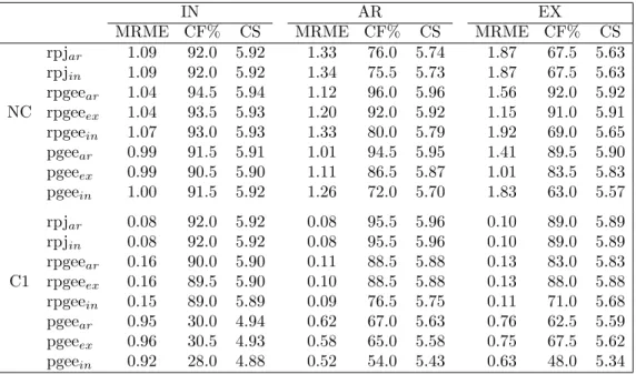
Study 2. In this study, we looked into the effect of covariance misspecification on mean estimation. We compared the performance of the robust penalized joint model, denoted rpj in Table 3, method with that of robust and non-robust penalized generalized estimating equations, denoted rpgee and pgee, methods that assume a fixed working correlation matrix and solve (2.2) for the mean. The most salient difference of the three methods is that our joint model builds regression models after decomposing the covariance matrix, while RPGEE and PGEE treat the covariance matrix as a nuisance and the marginal variance of yi is estimated from the sample. In PGEE, we set the tuning parameter of the Huber functioncas 1,000 and the weightW =I when solving (2.2) for the mean. Under the same mean set-up as in Study 1, we considered the covariance structures working independence (IN), auto-regressive (AR), and exchangeable (EX) with correlation parameter 0.5. We compared the performance of eight estimators: rpjar and rpjin are robust joint models with independent and AR(1) correlation structure assumptions for Cov(ε2i) in (2.4), respectively; rpgeeein, rpgeeear, and rpgeeeex (or pgeeein, pgeeear, and pgeeeex) are robust (or non-robust) penalized GEE estimations with IN, AR and EX as working correlation matrices. We adopted SCAD penalty in the study.
Table 3 lists the results under NC and C1. In the table, we employed MRME (the median of relative model error) to compare the performance of the eight estimators
ME (model error) of the estimator
ME of PGEE estimator with true covariance matrix.
In the absence of outliers (NC), in general, pgee estimators performed slightly better than rpgee estimators which in turn were better than the rpj estimators. Besides, rpjinand rpjar had similar performances, which suggests that the choice of the δ in (2.4) has little effect on the mean and covariance estimation. As a result, we fixed δ= 0 in a later application.
Table 3. Simulation results for Study 2.
IN AR EX
MRME CF% CS MRME CF% CS MRME CF% CS
rpjar 1.09 92.0 5.92 1.33 76.0 5.74 1.87 67.5 5.63 rpjin 1.09 92.0 5.92 1.34 75.5 5.73 1.87 67.5 5.63 rpgeear 1.04 94.5 5.94 1.12 96.0 5.96 1.56 92.0 5.92 NC rpgeeex 1.04 93.5 5.93 1.20 92.0 5.92 1.15 91.0 5.91 rpgeein 1.07 93.0 5.93 1.33 80.0 5.79 1.92 69.0 5.65 pgeear 0.99 91.5 5.91 1.01 94.5 5.95 1.41 89.5 5.90 pgeeex 0.99 90.5 5.90 1.11 86.5 5.87 1.01 83.5 5.83 pgeein 1.00 91.5 5.92 1.26 72.0 5.70 1.83 63.0 5.57 rpjar 0.08 92.0 5.92 0.08 95.5 5.96 0.10 89.0 5.89 rpjin 0.08 92.0 5.92 0.08 95.5 5.96 0.10 89.0 5.89 rpgeear 0.16 90.0 5.90 0.11 88.5 5.88 0.13 83.0 5.83 C1 rpgeeex 0.16 89.5 5.90 0.10 88.5 5.88 0.13 88.0 5.88 rpgeein 0.15 89.0 5.89 0.09 76.5 5.75 0.11 71.0 5.68 pgeear 0.95 30.0 4.94 0.62 67.0 5.63 0.76 62.5 5.59 pgeeex 0.96 30.5 4.93 0.58 65.0 5.58 0.75 67.5 5.62 pgeein 0.92 28.0 4.88 0.52 54.0 5.43 0.63 48.0 5.34
Simulation results of median of relative model error (MRME), average correctly fit percentage (CF%), and average numbers of regression coefficients that are correctly shrunk (CS) under NC (no contamination) and C1 (contamination), with 200 replications. rpjar and rpjinare robust joint models with independent and AR(1) correlation structure in (2.4), respectively; rpgeeein, rpgeeear, and rpgeeeex(or pgeeein, pgeeear, and pgeeeex) are robust (or non-robust) penalized GEE estimations with IN, AR, and EX as working correlation matrices.
Under C1, rpj estimators improved substantially over the rpgee and pgee estimators. Without the bounded score on the mean estimator, pgee mean esti-mators collapsed in any of the IN, AR or EX covariance structure, as all MRME’s for rpj and rpgee are less than 1 in C1. By adopting the robust estimator for the mean, rpgee estimators had reasonable performances on the mean estimation. However, rpj estimators further improved the performance of the mean estima-tor (variable selecestima-tor). Standard errors for the mean estimaestima-tors can be found in supplementary Table S3.2, which reveals the influence of outliers on the mean estimation.
Table S3.3 of the supplementary material lists entropy losses and quadratic losses on covariance matrix estimation. When there is no contamination, rpgee and pgee had comparable performances, and better than rpj. However, under C1, rpgee and pgee can be seriously affected by the contamination.
4. Data Analysis
has been analyzed be Fung et al. (2002), He, Zhu, and Fung (2002), Fan, Qin, and Zhu (2012), and Qin, Zhu, and Fung (2009). The data set contains 492 observations of progesterone level within a menstrual cycle, collected from 34 women clinical participants. In our model, the response variable yij is the log-transform of progesterone level and the observation time istij, apart from which patient’s age and body mass index (BMI) are recorded. Two objectives were considered when we implemented the robust variable selection method in the joint mean and covariance model to this hormone data set: to accommodate the influence of outliers and leverage points, and to detect outliers in the data set; to identify statistically significant covariates in linear models of both mean and covariance matrix.
The starting mean model we proposed was yij =β0+β1Agei+β2BM Ii+β3tij +β4t2ij
+β5Agei×BM Ii+β6Agei×tij +β7BM Ii×tij+eij
=xTijβ+eij.
For the covariance model, we followed the model in (1) and chose the correspond-ing covariates as
gijk= (1,(tij −tik),(tij −tik)2,(tij−tik)3)T, zij =xij.
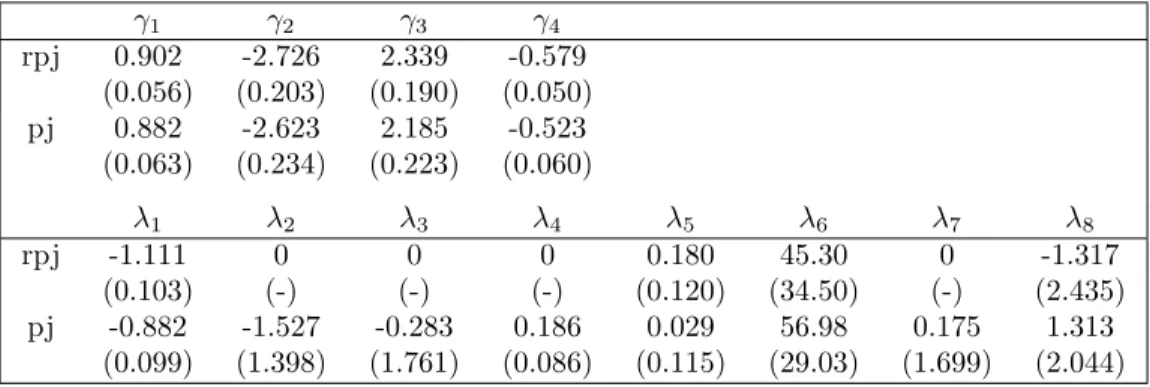
Three estimators were under consideration: rpj is the robust penalized joint model; pj is the penalized joint model proposed by Kou and Pan (2011); gee is the widely-used GEE estimator. Table 4 summarizes estimators of the mean parameters with standard errors. We noticed that the joint models (rpj and pj) are more parsimonious than gee as they choose time as the only significant variable. This is consistent with previous research that found that both Age, BMI, their interaction and interactions with time are not statistically significant in the model. We found that the regression coefficients for Time obtained by rpj and pj rather different, the non-robust pj estimator is affected by outliers.
Estimates with standard errors for the generalized autoregressive coefficients and innovation variances are summarized in Table 5. We found that the cubic polynomial of time is statistically significant for autoregressive coefficients γ in all fits. Standard errors in non-robust method are larger than those in the robust method. Unlike estimators of generalized autoregressive coefficients, significant covariates for innovation variances were not found in our analysis. Due to the existence of outliers, the non-robust method failed to select significant covariates for innovation variances.
Outlier detection was practiced with our procedure. By investigating the standardized residualssij and the weight functionwij, we found one observation-level outlier (observation 10) and one subject-observation-level leverage point (subject 18).
Table 4. Estimators of the mean parameters β and standard errors (inside brackets) for progesterone data.
Intercept Age BMI Time Time2 Age×BMI Age×Time BMI×Time
rpj 0.837 0 0 0.691 0 0 0 0 (0.074) (-) (-) (0.053) (-) (-) (-) (-) pj 0.892 0 0 0.562 0 0 0 0 (0.078) (-) (-) (0.056) (-) (-) (-) (-) gee 0.870 1.684 -2.671 0.709 0.186 -4.829 1.493 0.701 (0.126) (2.180) (2.928) (0.049) (0.085) (50.09) (0.827) (0.857)
In the table, rpj represents the robust penalized joint model; pj represents penalized joint model proposed by Kou and Pan (2011); gee is the traditional GEE estimator. Working independence is considered.
Table 5. Estimates of the generalized autoregressive parametersγand inno-vation variance parametersλfor progesterone data.
γ1 γ2 γ3 γ4 rpj 0.902 -2.726 2.339 -0.579 (0.056) (0.203) (0.190) (0.050) pj 0.882 -2.623 2.185 -0.523 (0.063) (0.234) (0.223) (0.060) λ1 λ2 λ3 λ4 λ5 λ6 λ7 λ8 rpj -1.111 0 0 0 0.180 45.30 0 -1.317 (0.103) (-) (-) (-) (0.120) (34.50) (-) (2.435) pj -0.882 -1.527 -0.283 0.186 0.029 56.98 0.175 1.313 (0.099) (1.398) (1.761) (0.086) (0.115) (29.03) (1.699) (2.044)
pij = (AGEi, BM Ii) contributed to the weight functions wij in our robust method. Subject 18 is a leverage point which had not been identified before; it has an extremely high BMI of 38 that heavily downweights the cluster of ob-servations from the patient. A careful inspection of the standardized residualsij tells us that case 10 is the most extreme point with sij = −6.09. The proges-terone level of the 10th observation for subject 1 (case 10) is 2.46, which is very different from its neighborhood observations 9 and 11 measured one day before and one day after. This inconsistency has not been noticed in the literature. All other thirteen observations of subject 1 range from 8.5 to 13.4 and in particular, this observation was the lowest progesterone level in the data set. We concluded that case 10 of subject 1 is a clear outlier. The influence of this outlier on the parameter estimates is detailed in Table S4.1 of the supplementary material. We also noticed that some observations have large standardized residuals, such as cases 117, 334 and 372, due to the fact that they are extreme values of the progesterone level within a subject. The effects on these potential outliers are downweighted by our robust method in the estimation of mean and covariance
parameters.
Acknowledgement
The authors are grateful to two reviewers, an associate editor, and the Co-Editor for their insightful comments and suggestions which have improved the manuscript significantly. This work was supported by the National Natural Sci-ence Foundation of China (10931002, 11271180).
References
Bickel, P. J. and Levina, E. (2008). Regularized estimation of large covariance matrices.Ann. Statist.36, 199-227.
Cantoni, E., Flemming, J. M. and Ronchetti, E. (2005). Variable selection for marginal longi-tudinal generalized linear models.Biometrics61, 507-514.
Cook, R. D and Weisberg, S. (1983). Diagnostics for heteroscedasticity in regression.Biometrika 70, 1-10.
El Karoui, N. (2008). Operator norm consistent estimation of large dimensional sparse covari-ance matrices.Ann. Statist.36, 2717-2756.
Fan, J., Huang, T., and Li, R. (2007). Analysis of longitudinal data with semiparametric esti-mation of covariance function.J. Amer. Statist. Assoc.35, 632-641.
Fan, J. and Li, R. (2001). Variable selection via nonconcave penalized likelihood and its oracle properties.J. Amer. Statist. Assoc.96, 1348-1360.
Fan, J. and Wu, Y. (2008). Semiparametric estimation of covariance matrices for longitudinal data.J. Amer. Statist. Assoc.103, 1520-1533.
Fan, Y. L., Qin, G. Y. and Zhu, Z. Y. (2012). Variable selection in robust regression models for longitudinal data.J. Multivariate Anal.109, 156-167.
Fu, W. J. (2003). Penalized estimating equations.Biometrics59, 126-132.
Fung, W. K., Zhu, Z. Y., Wei, B., and He, X. (2002). Influence diagnostics and outlier tests for semiparametric mixed models.J. Roy. Statist. Soc. Ser. B64, 565-579.
He, X., Fung, W. K., and Zhu, Z. Y. (2005). Robust estimation in generalized partial linear models for clustered data.J. Amer. Statist. Assoc.472, 1176-1184.
He, X., Zhu, Z. Y., and Fung, W. K. (2002). Estimation in a semiparametric model for longitu-dinal data with unspecified dependence structure.Biometrika89, 579-590.
Huang, J., Liu, N., Pourahmadi, M., and Liu, L. (2006). Covariance matrix selection and estimation via penalised normal likelihood.Biometrika93, 85-98.
Jeng, X. J. and Daye, Z. J. (2011). Sparse covariance thresholding for high-dimensional variable selection.Statist. Sinica21, 625-657.
Johnson, B., Lin, D. Y., and Zeng, D. (2008). Penalized estimating functions and variable selection in semiparametric regression models.J. Amer. Statist. Assoc.103, 672-680. Kou, C. and Pan, J. (2011). Variable selection for joint mean and covariance models via penalised
Likelihood, Technical report, Probability and Statistics Group School of Mathematics, The University of Manchester.
Leng, C., Zhang, W., and Pan, J. (2010). Semiparametric mean-covariance regression analysis for longitudinal data.J. Amer. Statist. Assoc.105, 181-193.
Liang, K. Y. and Zeger, S. L. (1986). Longitudinal data analysis using generalized linear models.
Biometrika73, 13-22.
Mao, J., Fung, W. K. and Zhu, Z. Y. (2011). Joint estimation of mean–covariance model for longitudinal data with basis function approximations. Comput. Statist. Data Anal. 55, 983-992.
Pan, W. (2001). Akaike’s information criterion in generalized estimating equations.Biometrics 73, 13-22.
Pourahmadi, M. (1999). Joint mean-covariance models with applications to longitudinal data: unconstrained parameterisation.Biometrika86, 677-690.
Pourahmadi, M. (2000). Maximum likelihood estimation of generalized linear models for multi-variate normal covariance matrix.Biometrika87, 425-435.
Qin, G. Y., Zhu, Z. Y., and Fung, W. K. (2009). Robust estimation of covariance parameters in partial linear model for longitudinal data.J. Statist. Plann. Inference139, 558-570. Qu, A., Lindsay, B., and Li, B. (2000). Improving generalised estimating equations using
quadratic inference functions.Biometrika87, 823-836.
Rothman, A. J., Levina, E., and Zhu, J. (2009). Generalized thresholding of large covariance matrices.J. Amer. Statist. Assoc.104, 177-186.
Xu, J. and Mackenzie, G. (2012). Modelling covariance structure in bivariate marginal models for longitudinal data.Biometrika99, 649-662.
Ye, H. and Pan, J. (2006). Modelling covariance structures in generalized estimating equations for longitudinal data.Biometrika93, 927-941.
Zheng, X. Y., Fung, W. K., and Zhu, Z. Y. (2013). Robust estimation in joint mean-covariance regression model for longitudinal data.Ann. Inst. Statist. Math.65, 617-638.
Zhou, J. and Qu, A. (2012). Informative estimation and selection of correlation structure for longitudinal data.J. Amer. Statist. Assoc.107, 701-710.
Zou, H. (2006). The Adaptive Lasso and its oracle properties. J. Amer. Statist. Assoc. 101, 1418-1429.
Department of Biostatistics, Fudan University, Shanghai, China. E-mail: [email protected]
Department of Statistics and Actuarial Science, The University of Hong Kong, Hong Kong. E-mail: [email protected]
Department of Statistics, Fudan University, Shanghai, China. E-mail: [email protected]