Mixed scale joint graphical
lasso
Pircalabelu E, Claeskens G, Waldorp L.
KBI_1616
Mixed Scale Joint Graphical Lasso
Eugen Pircalabelu1, Gerda Claeskens1,Lourens J. Waldorp2
1KU Leuven, ORSTAT and Leuven Statistics Research Center,
Naamsestraat 69, 3000 Leuven,Belgium
2University of Amsterdam, Department of Psychological Methods,
Weesperplein 4, 1018 Amsterdam, The Netherlands
Abstract
We develop a method for estimating brain networks from fMRI datasets that have not all been measured using the same set of brain regions. Some of the coarse scale regions have been split in smaller subregions. The proposed penalized estimation procedure selects undi-rected graphical models with similar structures that combine informa-tion from several subjects and several coarseness scales. Both within scale edges and between scale edges that identify possible connections between a large region and its subregions are estimated. Mixed scale data; Fused and Group lasso; Joint graphical lasso; ℓ1 penalization,
Sparsistency
1
Introduction
This work is motivated by the need to jointly estimate multiple undirected graphs from data that do not all have the same measurement scale. The example used here, originates from resting state functional magnetic reso-nance imaging (rsfMRI) where for two subjects brain activity measurements at voxel level were recorded. The rsfMRI images were segmented, first, in 68 atlas-based regions of interest (ROIs, i.e., sets of voxels that form non-overlapping parts of the brain), corresponding to a coarse measurement scale with anatomically large brain regions. Based on the procedure ofHagmann
and others (2008) several of the large ROIs were further split in two or more
smaller regions, resulting in a finer scale with 114 ROIs. For each subject, for all ROIs at each scale, n= 240 volumes of the blood oxygenation level dependent (BOLD) signal have been obtained. The researcher has knowl-edge about which ROIs have been split and a similar functional behavior for
a region and its subregions is expected. The setup bears some similarity to the multiresolution framework ofChoi and Willsky(2007);Choiand others (2010). However, by nature of the splitting process, the measurement for the coarse region cannot be algebraically reconstructed from the measurements of its subregions.
The objectives are twofold. First, we wish to jointly estimate sparse undirected graphs that show cerebral pathways between ROIs, where each ROI is associated with a node in the graph, using all the available data at coarse and finer scales. Analyzing data available at only one scale would make the implicit assumption that the chosen scale is in a sense ‘best’ and it has been shown that the definition of the ROIs has a high impact on the es-timated graph (see, e.g.Zaleskyand others,2010;Schmittmannand others,
2015). Our procedure avoids such a selection. To overcome the differences in the dimensionality between measurement scales, our procedure introduces two algebraic operators that make use of the knowledge which finer scale regions are subregions of a coarse scale region. Second, dependencies exist between a coarse scale node and its corresponding finer scale nodes due to the experimental design. This we refer to as ‘splits’. Our procedure is di-rected at estimating such splits. These splits are of interest because if the subregions are all connected, then it seems reasonable to assume that these subregions act as one, and so the region one scale up is good enough for modelling connectivity. In this sense estimating different scales simultane-ously with our proposed method indicates a data driven mixture of scales to use for modeling connectivity.
The graphs are estimated by enforcing sparsity viaℓ1-based penalization, studied for the estimation of undirected graphical models byYuan and Lin
(2007),Banerjeeand others (2008),Friedmanand others (2008),Bickel and Levina (2008a,2008b), Cai and others (2010) and Leng and Tang (2012) among others. See also B¨uhlmann and Van De Geer (2011) and Hastie
and others (2015) for a thorough treatment of regularization based on ℓ1
penalties and generalizations. Joint estimation of multiple sparse graphs has been studied by Guo and others (2011), Danaher and others (2014),
Gaskins and Daniels(2013),Zhaoand others (2014) andMohanand others (2014). For an overview, see alsoFanand others (2015).
We estimate graphs that show interactions between the regions both ‘within’ (to reveal brain pathways between ROIs) and ‘between’ coarseness scales (to reveal dependencies between coarser and finer nodes). The method can accommodate data from more than one subject, more than two measure-ment scales and an unequal numbers of splits for different ROI. Important for the method to work is the information on which regions have been split
and how many splits they have at each scale. We constrain the graphs for the different scales to be ‘similar’ to each other by using the ‘fused’ or ‘group’ graphical lasso penalties as inDanaherand others (2014). The cur-rent setting is diffecur-rent in that, first, their method requires to have the same measurement scale to combine graphs and, second, we allow for connections between the split and unsplit ROIs.
2
Notation
We associate to each random variable a node in an undirected graphG(E, V) where V ={1, . . . , p} represents the set of nodes andE is the set of undi-rected edgesi−j between a pair of nodes (i, j). A superscript denotes the measurement scale. Let X(k) be the random vector of variables that corre-spond to the ROIs for scalek, with length q(k). Whenk= 1, X(1) collects all variables at the coarse scale. All scales are splits of the coarsest scale. We call scalek > 1 finer than scale 1, or conversely scale 1 is coarser than scalek.
Define the vector X and its concentration matrix Θ, both partitioned according to the lengths q(k), k = 1, . . . , K, where the matrices Θkk are
the inverse covariance matrices corresponding to each of the K coarseness scales, while the matrices Θkk′ with k 6= k′ are the across-scale inverse covariance matrices between scales kand k′. If an element θi,j 6= 0 then an
edge links nodesiandjin the graphG(E, V) and there is thus, a one-to-one correspondence betweenΘand G(E, V),
X= (X(1)T,X(2)T, . . . ,X(K)T)T∼N(0,Σ), Σ−1≡Θ≡ Θ11 . . . Θ1K .. . . .. ... ΘK1 . . . ΘKK .
The goal is to estimate the matrices Θkk on the diagonal in such a way that they are sparse and ‘similar’ to each other, since they differ only in the measurement scale. The non-zero elements in Θkk are interpreted as the ‘within’ scale edges. The non-zero elements in the off-diagonal matrices
Θkk′ (k′6=k) are interpreted as the ‘between’ scale edges. The between scale graphs are constrained to be sparse as we only allow for the estimation of edges corresponding to splits of the same regions across the scales, i.e. coarse regioni is only allowed to connect to its subregions and not to subregions of another coarse region. Since we know exactly which regions are split, the sparsity pattern of the off-diagonal matrices is partially known, while this is unknown for the matrices on the diagonal.
(a) (b) (c)
Figure 1: Illustrative example involving ROIs 4 and 28 at two coarseness scales. Region 28 is split, first in 2, then in 3 subregions, whereas region 4 is unsplit at both scales. Panel (a) shows edges at the coarse scale, (b) shows edges at the fine scale and (c) shows edges between coarse regions and finer subregions.
Figure 1 shows an example using ROIs 4 and 28 at two scales. At both scales ROI 4 is unsplit, whereas ROI 28 is split first in two and next in three subregions. The matrixΘ11(within edges at the coarse scale) is represented in (a), (b) depictsΘ22. The between scale edges, or splits, contained inΘ12
are in (c). The goal is to estimate all these edges.
Denote by k ∈ {1, . . . , K} the coarseness scale, by h ∈ {1, . . . , H} a coarse ROI and byl ∈ {1, . . . , L} a partition of a coarse ROI, always used alongside region h. The couple {k, h(l)} denotes partition l of region h at scalek. In the example of Figure 1,{2,28(2)} refers to the second partition of ROI 28 at the second scale. There are K scales and H regions at the coarsest scale. The number of partitions within a scale is denoted by Lk
and can vary (e.g. at scale k = 3 we can have more splits of the region h
than at scale k = 2). The number of partitions can vary for each region (e.g.h′ can have more splits thanh). If a coarse ROI has not been split, the
region is used unchanged in the other scales.
The dimensions of each submatrix Θkk are dictated by the number of splits encountered at scale k and can be all different. To induce similarity between scales we couple a region that is split into, say, three regions at a finer scale to the original single region. This coupling requires that we have the same dimension in both scales (three in this case). To tackle this dimen-sionality problem we introduce in Section5the ‘expand’ operator which has the purpose of transforming all submatrices to a common dimension that is most informative.
We denote by the set W = {θi,jkk, k = 1, . . . , K;i, j = 1, . . . , q(k)} all el-ements of the block matrices on the main diagonal. If an element of W is non-zero, an undirected edge is present between different splits of dif-ferent regions within a scale. In the example of Figure 1(a)-(b), W corre-sponds to the parameters related to edges using nodes from a fixed scale. Define the set B = {θi,jkk′;k6=k′|i corresponds to h(l) and j corresponds to
h(l′),∀hand l, l′ = 1, . . . , L
k and k, k′ = 1, . . . , K} to contain all entries of
off-diagonal submatrices. In Figure 1(c), B corresponds to parameters re-lated to edges between the partitions of a ROI across scales. This reflects interest in parameters that (if non-zero) correspond to an undirected edge betweendifferent splits (landl′) of a region (h) across different scales (kand
k′). Only edges that relate to the same regions across scales are of interest
as they refer to the splits.
3
Estimation method
Since the number of nodes at each measurement scale is not the same due to the splitting, also the vector lengthsq(k),k= 1, . . . , K are different. As a first step, we bring all componentsX(k) to the same length by applying the ‘expand’ operator. When a certain coarse region has been split in, say, three subregions in its finest measurement scale, the expand operator repeats the measurement for that region three times. As a result, all expanded vectors have the same length. The mathematical details about this operator are given in Section5.
LetY = Ex(X, D) be the expanded vector based on the measurements X and the knowledge of the region splits D. For a sample Y1, . . . ,Yn,
denote bySExthe empirical variance matrix and letΣExbe the true variance matrix of Y. We minimize the following objective function
q(Ψ) =ntrace(SExΨ)−log detΨ+X
i6=j pλn1,λn2(|ψ 11 i,j|, . . . ,|ψi,jKK|) o , (1)
over symmetric positive definite matricesΨ, having the same dimension as
ΣEx and acting as a pseudo-concentration matrix sinceΣExis not invertible. Note thatΨ−1 6=ΣEx.
The penalty function pλn1,λn2 is a convex real valued function
depend-ing on two regularization values (λn1, λn2) that forces small entries to be shrunk to zero through λn1, while enforcing similarity between subgraphs
usepλn1,λn2(|ψ
11
i,j|, . . . ,|ψKKi,j |) to denote
pλn1,λn2(|ψ
11
i,j|, . . . ,|ψ1i,jK|,|ψ22i,j|, . . . ,|ψi,j2K|, . . . ,|ψKKi,j |).
To ensure similarity between the concentration submatrices Θkk, we use a ‘fused’ (FGL) or a ‘group’ (GGL) graphical lasso penalty as in Danaher
and others (2014). For the fused lasso penalty, see Tibshirani and others
(2005), H¨ofling and others (2010), Liu and others (2010) and Yang and
others (2015). The group lasso penalty has been introduced by Yuan and
Lin(2006) as a form of shrinkage that allows certain groups of parameters to be jointly estimated as zero or non-zero values. The two penalties in our context take the form,
pF GLλn1,λn2(|ψi,j11|, . . . ,|ψi,jKK|) = λn1 X k X k′ |ψi,jkk′|+λn2 X k X k′>k |ψi,jkk−ψi,jk′k′|, pGGLλn1,λn2(|ψi,j11|, . . . ,|ψi,jKK|) = λn1 X k X k′ |ψi,jkk′|+λn2{ X k (ψi,jkk)2}1/2,
where{ψ11i,j, . . . , ψi,jKK}are the elements in the expanded matrix that corre-spond to the unexpanded elements{θ11
i,j, . . . , θKKi,j } from the set W ∪ B. If
there is a ROI that has been split, the cardinality of{ψ11i,j, . . . , ψi,jKK}is larger than that of {θ11
i,j, . . . , θKKi,j }. For both penalties, the first term regularizes
all allowed edges (both within and between scales), while the second part, related toλn2, regularizes the similarity of the edges between the scales. All entries ofΨfor which the corresponding entries inΘare not inW ∪ B, are defined 0 due to only considering connections between ROIs and their split versions as enforced by the design.
FGL penalizes the differences between matrix entries, thus making them more similar to each other, while GGL allows entire groups of entries to be all zero or all non-zero. It encourages that non-zero entries of the concen-tration matrices occur at the same places. By setting entries to non-zero values at the same positions across the coarseness scales, the group penalty also enforces the within group matrices to be similar to each other. When the ordering of the scales is important, one might find the fused penalty more appropriate. When the group formed by the coarse regions and all its splits is of interest, rather than the ordering of the scales, then the group penalty might be more appropriate. Both penalties encourage shared spar-sity patterns across the different scales and as a consequence the matrices or rather their graph representations are close together. They have both been applied, so far, only for the case where one deals with the same scale of
coarseness, whereas we extend these ideas to different scales of coarseness. With the approach proposed in Danaher and others (2014) one cannot si-multaneously estimate several sparse graphs that allow between coarseness scale edges. Moreover, their technique is constructed for the case where the number of regions for both scales is the same, which for our problem is not the case, as we make a clear distinction between coarser and finer regions.
By optimizing (1) we obtain an estimated matrix which has a larger di-mension than desired. To bring all estimated matrices back to their original dimensions, we apply the ‘reduce’ operator on ˆΨ, see Section 5 for details. Roughly, if a coarse scale region is expanded in four subregions, the esti-mates for the four regions are combined in a (weighted) average, a single estimate, for the coarse scale region. We define the resulting reduced matrix as the mixed scale joint graphical lasso (msJGL) estimate of the concentra-tion matrix, since it jointly estimates the between and within scale edges across all coarseness scales.
4
Algorithm for the mixed scale joint graphical
lasso
The proposed algorithm, based on the ADMM algorithm presented inBoyd
and others(2011), allows one part of theΨmatrix to be estimated using the
FGL or GGL penalty, while the other part of the matrix is estimated using a regularℓ1 penalty. All off-diagonal elements ofΨcorresponding to the set
B receive only the ℓ1 penalty, while all elements of the submatrices on the main diagonal ofΨ, or equivalently the elements in the setW, receive both the ℓ1 penalty and either the group or fused penalty. The structural 0’s in the off-diagonal matrices are obtained by taking a large enough penalty such that all entries corresponding to unallowed edges in G(E, V) are set to zero. LetI and 0 be the identity and the null matrix of the appropriate dimension. The algorithm is described as follows.
Step 1: Apply the ‘expand’ operator to construct SEx and set ˆΨ = I, U =
0, Z=0.
Step 2: Update ˆΨ= arg minΨ(trace(SExΨ)−log detΨ+ ρ2||Ψ−Z+U||2F).
The solution is obtained in closed form. Compute the eigen decompo-sition ρ(Z−U)−SEx = QΛQT, where ρ > 0 is an arbitrary fixed scalar and form a diagonal matrix with entries ˜Xii ={eigi+ (eig2i +
4ρ)1/2}/(2ρ), where eigi is the i-th eigenvalue. Update ˆΨ=QXQ˜ T. Step 3: Split ˆΨ, U, Z into block matrices according to the number of scales.
Step 4: Update the block submatrices Zkk with k= 1, . . . , K , for which the FGL or GGL penalty is used,Zkk= arg minZkk
PK
k=1ρ2||Ψˆ
kk
−Zkk+ Ukk||2F +P
i=6 jpλn1,λn2(|zi,j11|, . . . ,|zi,jKK|). The Zkk can take different
values for the FGL and GGL penalties, but in both cases this amounts to applying the soft-thresholding operator on a linear combination of matrices.
Step 5: Update Zkk′ with k 6=k′ for which the ℓ1 penalty is used as Zkk
′
= Softλn1/ρ(Ψkk′ +Ukk′),where Softλn1/ρ is the soft-threshold operator usingλn1/ρas thresholding value.
Step 6: Update U = ˆΨ+U −Z and repeat steps 2-6 until convergence. Step 7: ‘Reduce’ ˆΨ to obtain ˆΘRed, the msJGL estimated concentration
ma-trix.
5
The Expand and Reduce operators
We denote by a◦b the elementwise and by a⊗b the Kronecker product between the vectors a and b. By 1q we denote a vector of length q with
elements equal to 1. The vector s(k) records for each coarsest region the number of splits at scalek. Letdh;h={1, . . . , H}be the maximal number of
edges that can be set between splits of a regionhfrom different measurement scales, hereby accounting for the hierarchical structure by only counting edges between consecutive scales. Let X((kh)) be the subvector of splits of region h for scale k. Further, let vh(k) = dh/#X((kh)), where the symbol #
denotes the number of elements in the vector.
Definition 1. Let X = (X(1)T,X(2)T, . . . ,X(K)T)T. Define a design
vec-tor D = s(1) ◦s(2) ◦. . .◦ s(K) ≡ (d1, d2, . . . , dH)T that records the
prod-uct of the number of splits across all coarseness scales. The expand op-erator produces the vector Ex(X,D) of length PH
h=1dhK, which is
de-fined asEx(X,D) = Ex(X(1),D),Ex(X(2),D), . . . ,Ex(X(K),D)T
where Ex(X(k),D) =(X((1)k)⊗1 v(1k)) T,(X(k) (2)⊗1v2(k)) T, . . . ,(X(k) (h)⊗1vh(k)) T, k= 1, . . . , K.
This operator ensures that all submatrices Ψkk′ have the same dimen-sion, which, in turn, allows to enforce similarity between coarse and finer scales, and to connect splits across scales.
Definition 2. Let Ψ be an expanded matrix and P a projection matrix of dimension PK k=1 PH h=1s (k) h × PH
to the length of the unexpanded vector X, while the number of columns corresponds to the length of the expanded vector Ex(X,D). Let ΘRed = Red(Ψ) =PΨPTbe the reduced matrix. P is constructed by placing1/v(hk)
on the row corresponding to the unexpanded region h from scale k and all the columns for the expanded region.
Using 1/v(hk)in the matrixP assigns equal weights to all splits of a region. Weighted averages where splits get different weights can be obtained by using other values. The matrixΘRed has the same dimension and structure asΘ. Only the entries that have been expanded in Ψ are reduced, as all other entries remain unchanged.
The reduce operator is not rank preserving, but has the properties that: (i) ΘRed contains a 0 on position (i, j) if all entries in Ψpertaining to the couple (i, j) are also 0 and (ii) if Ψ is symmetric and full rank, then also
ΘRedis a symmetric full rank matrix. Property (i) is similar to the ‘OR’ rule ofMeinshausen and B¨uhlmann(2006). If the entries in the expanded matrix are non-zero and do not cancel each other, then the reduced entry will also be non-zero. Property (ii) holds because the reduce operator is equivalent to applying elementary operations on the rows and columns of Ψ, which can be organized such thatΘRed becomes the upper-left submatrix and the off-diagonal blocks are each others transpose. Following Proposition 16.2 from Gallier (2011, pp. 435) if the matrixΨ is positive definite, alsoΘRed
is positive definite, implying full rank. The symmetry of ΘRed follows by that ofΨ.
6
Theoretical properties
Due to the eigenvalue decomposition of the expanded matrix, the complex-ity of the algorithm in Section4is of orderO (PH
h=1dhK)3
. Danaherand
others (2014) and Witten and others (2011) investigated improvements in
computational speed when the concentration matrix is block diagonal. In this case one can apply within each scale the FGL, GGL or graphical lasso (GL) on only a smaller subset of variables. A similar argument cannot be made for the msJGL, because of the design of the problem: the off-diagonal elements provide dependence information between larger and smaller parti-tions of the same anatomical ROI.
The ADMM algorithm is guaranteed to converge if the objective func-tion is closed, proper and convex (Assumpfunc-tion 1 inBoydand others,2011) and the Lagrangian of the objective function has a saddle point (their As-sumption 2). We make the same asAs-sumptions.
Let Sn = {(i, j)|ψkk
′0
i,j 6= 0;k, k′ = 1, . . . , K}, where the true expanded
matrix is Ψ0 = (ψkki,j′,0), and let sn = #Sn−pn denote the number of
off-diagonal non-zero elements in Sn. Let Φ0 ≡ (Ψ0)−1 be the inverse of
the pseudo-concentration matrix Ψ0. We stress that Φ0 is not a proper covariance matrix, but a pseudo-covariance matrix. Assume that: (a) there exist constants τ1 and τ2 such that 0 < τ1 <eigmin(Φ0) < eigmax(Φ0) <
τ2<∞; (b) the sequences
an= maxi,j∈Snmaxk,k′=1,...,K |p
′ λn,λn2(|ψ 11,0 i,j |, . . . ,|ψ KK,0 i,j |)| =O {(pn/sn+1+ 1)logpn/n}1/2
bn= maxi,j∈Snmaxk,k′=1,...,K |p
′′ λn,λn2(|ψ 11,0 i,j |, . . . ,|ψ KK,0 i,j |)| =o(1) and (c) for any non-random matrices A, B for which the operator norm
kAk = O(1), kBk = O(1), the quantity maxi,j | (A(SEx −Φ0)B)i,j |=
Op((logpn/n)1/2).
Condition (a) guarantees that the eigenvalues of Φ0 are well-behaved. The sequencean in condition (b) is connected to the bias of estimating
non-zero entries and represents the maximal value over indices (i, j) of any of the
K components in the partial derivative vector. And condition (c) mimics the result of Lemma 2 fromLam and Fan(2009) for the extended matrices.
Proposition 1. Under conditions (a)–(c) if (i) n−1logp
n = O(λ2n1) and (ii) (pn+sn)n−1(logpn)k =O(1) for some k >1, there exists a minimizer
ˆ
Ψsuch that ||Ψˆ −Ψ0||2F =O{(pn+sn)n−1logpn}.
Proposition 2. Under conditions (a)–(c) and conditions of Proposition 1 for any local minimizer that satisfies||Ψˆ−Ψ0||2F =OP{(pn+sn1)n−1logpn}
and||Ψˆ−Ψ0||2 =OP(ηn)for a sequenceηn→0, if the sequence{
p n−1log(p n)+ √η n +λn2 θkk i,j q PK k=1(θi,jkk)2 I(k = k′)} = O(λ
n1) for the GGL penalty or if
{p
n−1log(p
n) + √ηn+λn2Pk′′>ksgn(θkki,j −θk
′′k′′
i,j )I(k = k′)} = O(λn1) for the FGL penalty, then with probability tending to 1, ψˆkk′
ij = 0 for all
(i, j)∈Sc.
Proof. The proofs follow from Theorems 1 and 2 fromLam and Fan(2009) which follow the lines ofRothmanand others (2008) andBickel and Levina
(2008a, 2008b). We show that (i) P(infU∈Aq(Ψ0 +∆U) > q(Ψ0)) → 1 which implies that there exists a minimizer in the set
Ψ0+∆U :||∆U||2F ≤
C2
of ∂q(Ψ)
∂ψkk′
ij
wheni, j ∈Sc, depends only on sgn(ψkk′
ij ) which implies that∀k, k′
ˆ
ψijkk′ = 0 withi, j∈Snc with probability tending to 1.
For (i) it can be shown that q(Ψ)−q(Ψ0) can be decomposed as I1+
I2+I3, a sum which is asymptotically positive. For (ii) we can show that
ψkk i,j q PK k=1(ψkki,j)2 ≤1 and P k′′;k′′>ksgn(ψkki,j −ψk ′′k′′ i,j ) ≤K−1 (since it is a
finite sum, as K is fixed, of 1s or−1s). Ifψi,jkk′ lies in a small neighborhood of 0 (excluding the value 0), as long as the conditions of Proposition2 hold in the case of the GGL or FGL penalty, then the sign of the derivative will depend on the sign of ψkki,j′ only. This is because we can choose the
λn1 sequence to be large such that it dominates the remaining terms. This sparsistency rate implies that for entries that do not get the GGL/FGL penalty, the rate is pn−1log(p
n) +√ηn which is the same as for GL. For
entries that receive the GGL/FGL penalty, the rate is worse, due to the extra term associated withλn2.
7
Simulation study
We have evaluated the performance of msJGL against the performance of GL on seven measures:
(i) TPR= #estimated edges that are true edges
#true edges (true positive rate, larger
is better);
(ii) FPR= #edges that are NOT present in the true graph#estimated edges that are NOT true edges (false positive rate, smaller is better);
(iii) FDR= #estimated edges that are NOT true edges
#estimated edges (false discovery rate,
smaller is better);
(iv) SI= 1−#estimated edges#possible edges (sparsity index);
(v) SHD= #edge additions/deletions such that estimated graph = true graph (structural Hamming distance, smaller is better);
(vi) F1 = 2P R/(P +R) where P = #estimated edges that are true edges#estimated edges andR=T P R(F1 score,Jardine and van Rijsbergen,1971, larger is better); (vii) FL=||ΘˆRed−Θ||F = q Pp i=1 Pp j=1|θˆijRed−θij| 2, where p represents the number of columns of the matrixΘ(Frobenius loss, smaller is better).
Data corresponding to two different coarseness scales have been used for the simulation study. For the second scale, a graph with 300 or 600 nodes was generated. For the first scale, a graph with 1/3rd of this number of nodes
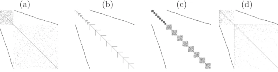
was generated, where each node was obtained from concatenating the ‘finer’ nodes from the second scale. The number of regions that were combined to obtain a coarser region varied randomly, meaning that some nodes were obtained by merging more regions than other nodes. Specifically, we have first sampled with replacement 300 indices from the set{1, . . . ,100} or 600 indices from the set {1, . . . ,200}, making sure that each integer from the set appeared at least once. The number of times an index appeared is how many finer nodes are combined to obtain the coarser node. For both scales the graph structure generated was either ‘random’, ‘hub’, ‘cluster’, ‘banded’ or ‘scale-free’. See Figure 2.
(a) (b) (c) (d)
Figure 2: Simulated data. Schematic representation of concentration ma-trices corresponding to four graphs used in the simulation study. For two scales a random (a), hub (b), cluster(c) or scale-free (d) graph has been generated. Black dots represent an edge between nodes, or equivalently a non-zero element in theΘmatrix. In each graph the ‘smaller’ bulk of points (bottom left) represents the graph for the first scale and the ‘larger’ bulk of points (top right) represents the graph for the second scale. The coarser regions of scale 1 have been split in finer regions on which the second scale has been measured. The splits are denoted by the two ‘lines’ above/below the diagonal.
From the composed graph we have defined aΣ−1 matrix as follows. The adjaceny matrix of the graph (that contained only 0 or 1 values, where 1 on rowiand columnj denotes the presence of an edge between nodesiand j) was multiplied with the value 3.9 and then an eigenvalue decomposition was performed. The diagonal values of the matrix were replaced by the absolute value of the minimal eigenvalue, to which the value 0.4 was added to ensure positive definiteness. Withn either 100, 300 or 3000, data were generated from a normal distribution, of mean vector 0 and with Σ as covariance matrix. Note that as in the real example from Section 8 both graphs are available for all the samples. The number of simulation runs was set at 500. Both msJGL and GL use the ADMM algorithm in the optimization process.
In the GL case, we estimate from the data two separate graphs (corre-sponding to each scale) using for each of them a separate graphical lasso. Note that there is no involvement of the reduce/expand operators when us-ing GL and note too that the estimated graphs based on GL do not take into account any desire of obtaining graphs that are similar to each other, nor do they account that some nodes in the larger graph are actually ob-tained from splitting nodes in the coarser graph; as such GL is insensitive to dependencies induced by splits.
FPR TPR 0 .5 1 0 .25 .5 GL msJGL λ2=.001 msJGL λ2=.003 msJGL λ2=.007 msJGL λ2=.01 msJGL λ2=.05 FDR msJGL FDR GL 0 .5 1 0 .5 1 λ2=.001 λ2=.003 λ2=.007 λ2=.01 λ2=.05 SI msJGL SI GL .4 .7 1 .4 .7 1 λ2=.001 λ2=.003 λ2=.007 λ2=.01 λ2=.05 F1 msJGL F1 GL 0 .5 1 0 .5 1 λ2=.001 λ2=.003 λ2=.007 λ2=.01 λ2=.05 SHD msJGL SHD GL 0 400000 0 200000 400000 λ2=.001 λ2=.003 λ2=.007 λ2=.01 λ2=.05 FL msJGL FL GL 200 600 1000 200 600 1000 λ2=.001 λ2=.003 λ2=.007 λ2=.01 λ2=.05
Figure 3: Simulated data. The panels present the TP rate against FP rate, FD rate, Sparsity index (top row) and F1 score, Hamming distance and Frobenius loss (bottom row) for msJGL and GL.
Figure 3 presents the obtained results. Each symbol represents the av-erage over all simulation runs within one simulation setting, where a certain
p,n,λn1,λn2 and penalty was used. For this study bothλn1and λn2 take a value in the fixed set{.001, .003, .007, .01, .05}and once aλn1 is selected, then it is used for both msJGL and GL. For the FDR, SHD and FL plots, a value above the diagonal indicates a more favorable position of msJGL against GL. For theF1 and SI plots, a value below the diagonal indicates a more favorable position of msJGL against GL.
pro-vided larger TP rates. For ease of exposition, Figure3(top left panel) shows the TPR and FPR performance for the case where the number of nodes was 800 (200 coarse scale nodes and 600 finer scale nodes), the sample size was 300 and the FGL penalty was used. For each of the 5 types graphs a curve is presented. Similar behavior was observed for the other settings and when using the group penalty. In a large majority of cases the SHD,F1 and FDR measures were either comparable or better for msJGL. With respect to the Frobenius loss, the results indicate that the performance is either compara-ble to that of the graphical lasso or slightly worse due to the constraint of the similarity of submatrices which forces entries in the concentration matrix to have similar values. In general, increasing theλn2 regularization parameter has as a direct effect a slight improvement in the performance, increasing in the same time the sparsity of the msJGL graph as this increases the regular-ization imposed on the estimated concentration matrix. Whileλn1 involves shrinking single entries in the concentration matrix, λn2 influences groups of parameters.
8
rsfMRI example
For two subjects that were instructed to stay alert and focus on a white fixation cross, rsfMRI data were acquired. The obtained images at scale 1 were segmented into 68 atlas-based ROIs, while for the second scale 114 atlas-based ROIs have been used (Desikanand others,2006). The 68 ROIs correspond to a coarser scale of measurement which implies that the brain regions under investigation were anatomically larger. In the second step, some of the large regions were further split into several smaller regions, resulting in a total of 114 ROIs for which the cerebral activity has been measured. For all ROIs we obtained n = 240 volumes of the BOLD sig-nal. See Schmittmann and others (2015) for more information regarding the acquisition of the data.
We want to investigate: (i) if there are links present in the estimated networks due to the splitting of regions between scales, that connect coarser regions with their smaller counterparts; (ii) which links are present between regions within a given coarseness scale. To answer these questions, we have applied the msJGL algorithm to the data from both subjects using the FGL and GGL penalties on a grid of regularization parameters (λn1,λn2). The final regularization parameters have been selected to convey sufficient information about brain pathways without having the graphs too cluttered, nor having them too sparse. A cross-validation scheme or an information
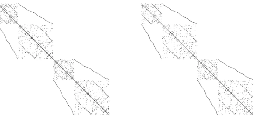
Figure 4: fMRI data. Schematic representation of estimated concentration matrices with the fused (left panel) and group (right panel) msJGL proce-dure using (λn1, λn2) = (.4, .1). The black dots represent an edge between nodes, or equivalently a non-zero element in the estimated concentration matrix. The square ‘bulks’ of points denote the within coarseness scale edges, while the ‘lines’ above/below the diagonal denote the between scale edges. Each panel represents two subjects with two scales (coarse and fine). criterion-based selection could also have been used to select an appropriate regularization value.
Figure 4 shows that both the FGL and GGL estimated between scale edges (‘split’ dependencies) as most of the entries are non-zero. This suggests that conditional independencies between the coarser and finer scale splits, are not supported by the data.
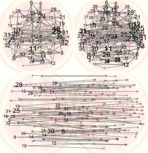
Figure 5 presents both the common and the unique edges pertaining to the estimated graphs for both subjects at each scale (upper row) and the estimated splits across the scales (bottom row). The graphs appear stable across subjects, which is seen by the percentage of common edges within scales (97.9% for the coarse scale and 98.2% for the fine scale) and between scales (93.7%). Our method explicitly estimates the splits, and provides information on how the different scales are functionally related. Here we can see that most differences between the subjects within and between scales are in the parietal and prefrontal areas. This is in line with poorer reliability in these brain areas as found inMueller and others (2015).
It is striking that the coarser regions do not connect with some of the finer subregions. The coarser regions connect at most to one or two finer subregions, indicating that some of the coarser regions are formed by
group-Figure 5: fMRI data. Fused msJGL within scale (top row) and between scale (bottom row) graphs. Both the coarse scale (top left) and the fine scale (top right) are presented. Full line edges are common edges for both subjects, while dashed and dot-dashed edges are estimated for one subject, but not for the other. The values of the regularization parameters are (λn1, λn2) =
(.4, .1).
ing together several heterogeneous finer subregions. This would indicate that the function of one or more subregions is different. This is likely to be found in rather arbitrary parcellations (Zaleskyand others,2010). This is the case for ROIs 23, 29 and 30. The most extreme case is that of the
coarse ROI 29, which for one subject connects to only one split, although the left and right hemispheres contained each four splits, suggesting that this coarser region is a conglomerate of regions that exhibit different cerebral activity. On the other hand regions 8, 9, 10, 12, 13, 14, 16, 30 and 32 from the left hemisphere, as well as regions 7, 8, 9, 10, 12, 16, 31 and 32 from the right hemisphere seem to be homogeneous regions, as links are present between the coarser regions and all of their finer splits.
The impact of using either a group or fused penalty can be important for the estimated structure and sparsity of the networks, but there is an agreement with respect to which regions are deemed important. Regions 10, 24, 25, 26, 28, 29, 31 and 32 are highly connected (see Figure 5) with the rest of the ROIs for both scales and both penalties.
The analysis was performed on a standard laptop. As a test, we let the algorithm perform 1000 iterations, which took around 2 minutes when applied to one subject and about 86 minutes for two subjects. In both cases two coarseness scales have been used.
9
Discussion
We have developed a new method of jointly estimating graphs where the nodes come from mixed coarseness scales. The approach is motivated by an fMRI dataset where the brain image has been ‘partitioned’ in various regions of interest in an incremental manner. The cerebral activity has been measured first, for 68 ROIs and then for 114 ROIs, where the latter, finer ROIs were created by splitting the coarser ROIs. Using the proposed method we were able to identify certain brain regions which exhibit either a homogeneous or heterogeneous cerebral activity pattern. The method has direct applicability beyond fMRI data, in other areas where data on different scales are observed and where the joint estimation of graphs that resemble each other is desired.
Having multiple coarseness scales, sets as an open problem the identifi-cation of an optimal coarseness scale of the data at which a scientist should perform the analysis. Different scales lead to some qualitative differences in the conclusions, but one would hope that the decision on the scales is invari-ant. Such questions related to the selection of an optimal coarseness scale are the subject of ongoing research. The proposed method avoids selecting one such optimal scale and produces interpretable results at all available scales.
Acknowledgements
The authors wish to thank the reviewers for their constructive comments. E. Pircalabelu is postdoctoral researcher of the Research Foundation Flan-ders (FWO) of which the support is acknowledged, together with support from KU Leuven grant GOA/12/14, and of the IAP Research Network P7/06 of the Belgian Science Policy. The computational resources and services used in this work were provided by the VSC (Flemish Supercomputer Center), funded by the Hercules Foundation and the Flemish Government - depart-ment EWI.
References
Banerjee, O., El Ghaoui, L. and d’Aspremont, A. (2008). Model selection through sparse maximum likelihood estimation for multivariate Gaussian or binary data. Journal of Machine Learning Research 9, 485– 516.
Bickel, P. J. and Levina, E. (2008a). Covariance regularization by thresholding. The Annals of Statistics 36(6), 2577–2604.
Bickel, P. J. and Levina, E. (2008b). Regularized estimation of large covariance matrices. The Annals of Statistics 36(1), 199–227.
Boyd, S., Parikh, N., Chu, E., Peleato, B. and Eckstein, J.(2011). Distributed optimization and statistical learning via the alternating direc-tion method of multipliers. Foundations and Trends in Machine Learn-ing 3(1), 1–122.
B¨uhlmann, P. and Van De Geer, S. (2011). Statistics for High-Dimensional Data: Methods, Theory and Applications. Springer.
Cai, T. T., Zhang, C.-H. and Zhou, H. H.(2010). Optimal rates of con-vergence for covariance matrix estimation.The Annals of Statistics.38(4), 2118–2144.
Choi, M.J., Chandrasekaran, V. and Willsky, A.S.(2010). Gaussian multiresolution models: exploiting sparse Markov and covariance struc-ture. IEEE Transactions on Signal Processing 58(3), 1012–1024.
Choi, M.J and Willsky, A.S. (2007). Multiscale Gaussian graphical models and algorithms for large-scale inference. In: Statistical Signal Processing, 2007. SSP ’07. IEEE/SP 14th Workshop on. pp. 229–233.
Danaher, P., Wang, P. and Witten, D. (2014). The joint graphical lasso for inverse covariance estimation across multiple classes. Journal of the Royal Statistical Society, Series B, 76(2), 373–397.
Desikan, R. S., S´egonne, F., Fischl, B., Quinn, B. T., Dickerson, B. C., Blacker, D., Buckner, R. L., Dale, A. M., Maguire, R. P., Hyman, B. T., Albert, M. S.and others. (2006). An automated label-ing system for subdividlabel-ing the human cerebral cortex on MRI scans into gyral based regions of interest. NeuroImage 31(3), 968 – 980.
Fan, J., Liao, Y. and Liu, H. (2015). An overview on the estimation of large covariance and precision matrices. Technical report.
Friedman, J., Hastie, T. and Tibshirani, R. (2008). Sparse inverse covariance estimation with the graphical lasso. Biostatistics 9(3), 432– 441.
Gallier, J.(2011). Geometric Methods and Applications: For Computer Science and Engineering. Springer.
Gaskins, J. T. and Daniels, M. J. (2013). A nonparametric prior for simultaneous covariance estimation. Biometrika 100(1), 125–138.
Guo, J., Levina, E., Michailidis, G. and Zhu, J. (2011). Joint esti-mation of multiple graphical models. Biometrika 98(1), 1–15.
Hagmann, P., Cammoun, L., Gigandet, X., Meuli, R., Honey, C. J., Wedeen, V. J. and Sporns, O. (2008). Mapping the structural core of human cerebral cortex. PloS Biology 6(7), e159.
Hastie, T., Tibshirani, R. and Wainwright, M. (2015). Statisti-cal Learning with Sparsity: The Lasso and Generalizations, Chapman & Hall/CRC Monographs on Statistics & Applied Probability. Taylor & Francis.
H¨ofling, H., Binder, H. and Schumacher, M. (2010). A coordinate-wise optimization algorithm for the fused lasso. Technical Report.
Jardine, N. and van Rijsbergen, C.J.(1971). The use of hierarchic clus-tering in information retrieval. Information Storage and Retrieval 7(5), 217–240.
Lam, C. and Fan, J.(2009). Sparsistency and rates of convergence in large covariance matrix estimation. The Annals of Statistics 37(6B), 4254– 4278.
Leng, C. and Tang, C. Y.(2012). Sparse matrix graphical models. Jour-nal of the American Statistical Association 107(499), 1187–1200.
Liu, J., Yuan, L. and Ye, J.(2010). An efficient algorithm for a class of fused lasso problems. In: Rao, B., Krishnapuram, B., Tomkins, A. and Qiang, Y. (editors),KDD. pp. 323–332.
Meinshausen, N. and B¨uhlmann, P. (2006). High-dimensional graphs and variable selection with the lasso. The Annals of Statistics 34(3), 1436–1462.
Mohan, K., London, P., Fazel, M., Witten, D. and Lee, S. (2014). Node-based learning of multiple Gaussian graphical models. Journal of Machine Learning Research 15(1), 445–488.
Mueller, S., Wang, D., Fox, M. D., Pan, R., Lu, J., Li, K., Sun, W., Buckner, R. L. and Liu, H.(2015). Reliability correction for functional connectivity: Theory and implementation. Human brain mapping36(11), 4664–4680.
Rothman, A. J., Bickel, P. J., Levina, E. and Zhu, J.(2008). Sparse permutation invariant covariance estimation. Electronic Journal of Statis-tics 2, 494–515.
Schmittmann, V. D., Borsboom, D., Jahfari, S., Savi, A. and Wal-dorp, L. J. (2015). Making large-scale networks from fMRI data. PLoS One 10(9), e0129074.
Tibshirani, R., Saunders, M., Rosset, S., Zhu, J. and Knight, K. (2005). Sparsity and smoothness via the fused lasso. Journal of the Royal Statistical Society, Series B, 67(Part 1), 91–108.
Witten, D. M., Friedman, J. H. and Simon, N.(2011). New insights and faster computations for the graphical lasso.Journal of Computational and Graphical Statistics 20(4), 892–900.
Yang, S., Lu, Z., Shen, X., Wonka, P. and Ye, J. (2015). Fused multiple graphical lasso. SIAM Journal on Optimization 25(2), 916–943. Yuan, M. and Lin, Y.(2006). Model selection and estimation in regression with grouped variables. Journal of the Royal Statistical Society, Series B,68, 49–67.
Yuan, M. and Lin, Y. (2007). Model selection and estimation in the Gaussian graphical model. Biometrika 94(1), 19–35.
Zalesky, A., Fornito, A., Harding, I.H., Cocchi, L., Y¨ucel, M., Pantelis, C. and Bullmore, E. T. (2010). Whole-brain anatomical networks: does the choice of nodes matter? Neuroimage 50(3), 970–983. Zhao, S. D., Cai, T. T. and Li, H. (2014). Direct estimation of
FACULTY OF ECONOMICS AND BUSINESS Naamsestraat 69 bus 3500 3000 LEUVEN, BELGIË tel. + 32 16 32 66 12 fax + 32 16 32 67 91 [email protected] www.econ.kuleuven.be