HAL Id: hal-02373338
https://hal.archives-ouvertes.fr/hal-02373338v3
Submitted on 22 Nov 2019HAL is a multi-disciplinary open access archive for the deposit and dissemination of sci-entific research documents, whether they are pub-lished or not. The documents may come from teaching and research institutions in France or abroad, or from public or private research centers.
L’archive ouverte pluridisciplinaire HAL, est destinée au dépôt et à la diffusion de documents scientifiques de niveau recherche, publiés ou non, émanant des établissements d’enseignement et de recherche français ou étrangers, des laboratoires publics ou privés.
Multi-Task Learning for Neural Networks
Amaury Bouchra Pilet, Davide Frey, François Taïani
To cite this version:
Amaury Bouchra Pilet, Davide Frey, François Taïani. Simple, Efficient and Convenient Decentralized Multi-Task Learning for Neural Networks. 2019. �hal-02373338v3�
Learning for Neural Networks
Amaury Bouchra Pilet, Davide Frey and François Taïani 1 Frimaire 228
Abstract
Artificial intelligence relying on machine learning is increasingly used on small, personal, network-connected devices such as smartphones and vocal assistants, and these applications will likely evolve with the development of the Internet of Things. The learning process requires a lot of data, often real users’ data, and computing power. Decentralized machine learning can help to protect users’ privacy by keeping sensitive training data on users’ devices, and has the potential to alleviate the cost born by service providers by off-loading some of the learning effort to user devices. Unfortunately, most approaches proposed so far for distributed learning with neural network are mono-task, and do not transfer easily to multi-tasks problems, for which users seek to solve related but distinct learning tasks and the few existing multi-task approaches have serious limitations. In this paper, we propose a novel learning method for neural networks that is decentralized, multi-task, and keeps users’ datalocal. Our approach works with different learning algorithms, on various types of neural networks. We formally analyze the convergence of our method, and we evaluate its efficiency in different situations on various kind of neural networks, with different learning algorithms, thus demonstrating its benefits in terms of learning quality and convergence.
I Introduction
A critical requirement for machine learning is training data. In some cases, a great amount of data is available from different (potential) users of the system, but simply sharing this data and using it for training is not always the best solution. This significantly increases the amount of computation that has to be done on one single system, since all this data would then be processed on one system at a time. It may require high amounts of communication if the dataset is large. Also, users may not be willing to share their data because it is sensitive. For example, data from healthcare centers can be used to train neural networks to predict patients possible diseases [Che+17], but this data is very sensitive.
To address these issues, several works have proposed to share model-related information (such as gradients or model coefficients) rather than raw data [Rec+11; Kon+16; Bre+17]. However, the problems that users want to solve may not be perfectly identical. For example, in speech recognition, every one has a different voice and thus, all systems performing speech recognition do not exactly perform the same task. Also, in some cases, some classification can be done among users, for example, still in speech recognition, french-speaking users, users from Quebec can clearly be separated from users from France.
Although several approach have looked at distributed multi-task learning, they are typically limited to ether linear [OHJ12] or convex [Smi+16; Bel+18; ZBT19] optimization problems, and are not generally applicable to neural networks.
To the best of our knowledge, the only existing solution for distributed multi-task learning that is applicable to neural networks [CB19] relies on a client-server model, and is incompatible with a
decentralized setup. Moreover, the algorithm presented is sequential, not parallel, which negates the speed gain from distribution and make this method very poorly scalable.
This paper introduces an effective solution for decentralized multi-task learning with neural net-works. This method is usable in decentralized or federated setups, applicable to different training algorithms, keeps data local and effectively parallel. It also not requires mandatory prior knowledge about the nature, nor magnitude, of the differences between tasks, while still being able to benefit from such knowledge when available.
II The method
II.1 Base system model
Each peer𝑝has a neural network𝑁𝑝and data provider𝐷𝑝. 𝑁𝑝.train(𝐷𝑝)means that the network
is trained using𝐷𝑝(the training algorithm can be anything). 𝑁𝑝.test(𝐷𝑝) means that the network is
tested using 𝐷𝑝, and returns a∈ ℝ+ success rate. Each peer seeks to maximize the success rate of its
neural network when tested with its data provider.
Each neural network 𝑁𝑝 is divided into parts (one or more) of neurons having identical input
(with different weights), activation function (with different parameters) and with their outputs treated equivalently: 𝑁𝑝= (𝑁𝑝
0, …, 𝑁 𝑝
𝑘)1. The essential idea of a part is that neurons in a part can be treated
equivalently and permuted without altering the computation. This corresponds, for example, to a fully connected layer, but not to a convolutional layer [LB95], which must be divided into several parts. Parts consist of several neurons and an associated activation function: 𝑁𝑖𝑝 = ((𝑁𝑖,0𝑝 , …, 𝑁𝑖,𝑘𝑝 ), 𝑓)
(Theoretically this definition is actually equivalent to having specific activation functions for each neuron, since a real parameter can be used to index activation functions in a finite set of neurons)2.
The activation function 𝑓 is a real function with real parameters ℝ × ℝ𝑘 → ℝ. Each neuron 𝑛(𝑛 is
used instead of𝑁𝑖,𝑘𝑝 for readability) consists of a weight vector and an activation function parameters vector, both are real𝑛 = (w,q) ∈ ℝ𝑗× ℝ𝑘. wand qmay be learned by any training method. Neurons
take an input vector i∈ ℝ𝑘 and return a real value𝑓(i⋅w,q).
The neurons of a part all have the same input (but some input coordinates may have a fixed 0
weight, as long as this is also the case for all coordinates averaged with them), which can be either the output of another part or the input of the network itself. For modeling, we consider that the input arrives at designated input parts, consisting of neurons which just reproduce the input and are not updated in training. Bias neurons, outputting a constant value, are not considered, since their behavior is equivalent to introducing a bias as activation function parameter. Since they have fixed parameters, input parts are implicitly excluded from the collaborative learning process, since they simply do not learn.
A peer’s neural network may include parts that do not exist for all peer’s networks.
II.2 General idea
Based on the model averaging idea used for federated learning as proposed in [Bre+17], we devel-oped a method to allow multi-task learning in a decentralized setup.
Our original intuition is that similar but different tasks can be divided in two sections: a common section and an individual section. Based on this, we propose that neural networks could achieve multi-task learning if they were themselves divided in two: a general section that uses collaborative learning, and a local section, that learns purely locally.
1𝑖,𝑗and𝑘are used as generic index variables. Unless explicitly stated otherwise,𝑖,𝑗and𝑘from different formulas have not the same meaning
2#ℝ = ℶ
1 > ℶ0 = ℵ0 > 𝑘(∀𝑘∈ℕ), since the set of neurons is finite, it is not an issue to use a real index to define each neuron’s activation function, even if#ℝℝ= ℶ
2> ℶ1= #ℝimplies that a real value can not index the set of all real functions
Figure 1: Parts (dashed rectangles) and slices (nodes (neurons) of same color and shape) We present a generalized version of this idea. Since different peers involved in multi-task learning may have more or less similar functions to learn, it is interesting to also have portions of neural networks that are averaged between only a subset of the peers. So, we propose to divide neural networks into several sections, each to be averaged with a specific subset of the peers. We refer to such sections as slices.
In the following, we provide a formal description of our method.
II.3 Detailed approach
We define slices as disjoint sets of neurons that cover the entire neural network: 𝑁𝑝 = ⨄ 𝑖𝑆
𝑝,𝑖,
where𝑆𝑝,𝑖 is a slice. Each slice consists of a portion of a neural network that is averaged on a specific
subset of peers. Figure 1 gives and example of neural network divided into parts (dashed rectangles) and slices (nodes (neurons) of same color and shape).
We also introduce partial models. A partial model essentially consists of the model implemented by the neurons in a given slice of a neural network. Slices of different peers with identical sizes may implement the same partial model. Specifically, we classify models into three categories. A global model consists of a partial model shared by all the peers (without loss of generality we can consider that there exists only one global model). A semi-local model consists of a partial model shared by several but not all peers, while alocal model consists of a partial model associated with only one peer. Without loss of generality we can view all global (local) models of a peer as a single global (local) one. A peer has at least one model of any type, but none of the types is required.
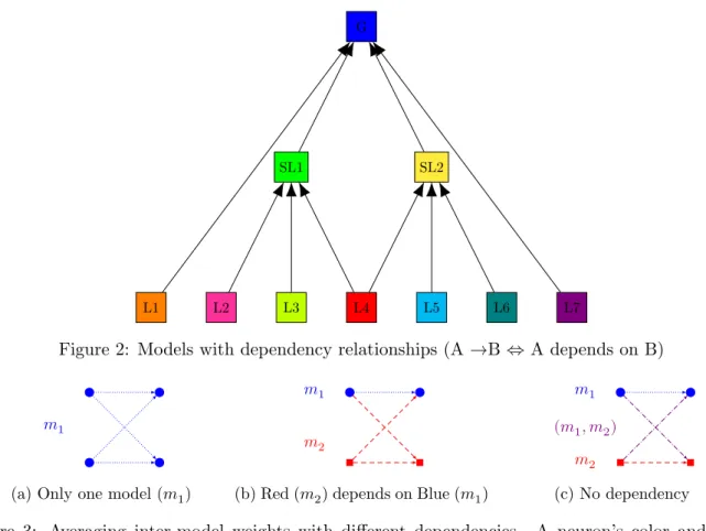
We also define a notion of dependencies between partial models: for example a partial model that recognizes Quebecois French may depend on a model that recognizes generic French. If a peer implements a partial model (associating it with one of its slices) it must also implement all the models on which it depends. This allows us to determine how to average inter-model weights. An example of models of different types with dependency relationships is given in Figure2(boxes ares partial models, arrows are dependency relationships).
II.3.a Partial averaging
Partial models allow us to implement partial averaging, as opposed to global averaging of the whole neural network, as done in non-multi-task collaborative learning. For each partial model, we only average the slices associated with it at the different peers that implement it.
When averaging the slices associated with a partial model, we average all the activation-function parameter vectors,qentirely, of associated neurons, and a subset of the input weights (a subset of each
G
SL1 SL2
L1 L2 L3 L4 L5 L6 L7
Figure 2: Models with dependency relationships (A →B⇔ A depends on B)
𝑚1
(a) Only one model (𝑚1)
𝑚1 𝑚2
(b) Red (𝑚2) depends on Blue (𝑚1)
𝑚1
(𝑚1, 𝑚2) 𝑚2
(c) No dependency
Figure 3: Averaging inter-model weights with different dependencies. A neuron’s color and shape indicates the model associated with the neuron; an edge color and style indicates for which model this edge weight will be averaged. We represent two models: blue circles and dotted lines versus red squares and dashed lines. Purple edges refers to weights that are not averaged in either model. in the same slice. For inter-model input weights, we rely on the notion of dependencies between partial models. Specifically, we average only the inter-model weights that connect a model to the models it depends on. The dependency ensures that these weights have the same meaning for all the peers implementing the model. For example, in Figure 3b, the red model can be Quebecois, while the blue model may be French. We average the inter-model weights among the peers that implement the Quebecois model. If there is no dependency between two models (Figure3c) the inter-model weights remain local to each peer. It is possible to average such weights among all peers that implement both partial models at the same time. But this would add significant complexity to the process for limited gain.
II.3.b Algorithm
In the following algorithms, 𝑝 ⊩ 𝑚 means that peer 𝑝 implements model 𝑚, 𝑛 ⋐ 𝑚 (resp. 𝑘 ⋐ 𝑚) means that the neuron 𝑛 (resp. indexed by 𝑘) is part of the (implementation of) model 𝑚.
𝑚.𝑑𝑒𝑝𝑠 is the dependencies of model𝑚. The notation 𝑛 ⋐ 𝑚.𝑑𝑒𝑝𝑠 (resp. 𝑘 ⋐ 𝑚.𝑑𝑒𝑝𝑠) is a short for ⋁
𝑚′∈𝑚.𝑑𝑒𝑝𝑠𝑛 ⋐ 𝑚
′ (resp. ⋁
𝑚′∈𝑚.𝑑𝑒𝑝𝑠𝑘 ⋐ 𝑚
′).
For simplification, this formalization does not address index differences between peers for equivalent neurons (or parts, if they are not identical for all peers) and use𝑇for the set of all parts and𝑇𝑖for the set of all neurons of a part. This issue can be addressed in implementation by adding indices offsets values for each model and each peer.
Algorithm1describes our distributed multi-task learning method. Algorithm2presents a modified main loop (and an additional function) to allow cross-model averaging.
Algorithm 1:Decentralized multi-task learning
Data: 𝑛𝑢𝑚number of peers,𝑚𝑏𝑛 number of training rounds between averaging,𝑀, the set of all models, 𝑇,𝑁 and 𝐷as defined before
1 loop
2 each peer0 ⩽ 𝑝 < 𝑛𝑢𝑚 does
3 for0 ⩽ 𝑖 < 𝑚𝑏𝑛do
4 𝑁𝑝.TRAIN(𝐷𝑝)
5 foreach𝑚 ∈ 𝑀 do
6 AVERAGEMODEL({𝑝 ∈ [0, 𝑛𝑢𝑚[|𝑝 ⊩ 𝑚},𝑚) // Does nothing if model 𝑚 is local 7 function AVERAGEMODEL(𝑃,𝑚) is 8 foreach𝑖 ∈ 𝑇 do 9 foreach𝑘 ∈ 𝑇𝑖|𝑘 ⋐ 𝑚 do 10 AVERAGE({𝑁𝑖,𝑘𝑝 .q|𝑝 ∈ 𝑃 }) 11 AVERAGERESTRICTED({𝑁𝑖,𝑘𝑝 .w|𝑝 ∈ 𝑃 },{𝑗|𝑗 ⋐ 𝑚 ∨ 𝑗 ⋐ 𝑚.𝑑𝑒𝑝𝑠}) 12 foreach𝑘 ∈ 𝑇𝑖|𝑘 ⋐ 𝑚.𝑑𝑒𝑝𝑠 do 13 AVERAGERESTRICTED({𝑁𝑖,𝑘𝑝 .w|𝑝 ∈ 𝑃 },{𝑗|𝑗 ⋐ 𝑚})
elements of a set of vectors, the second average predefined coordinates (second parameter) of vectors from a set (first parameter). In a decentralized setup, those functions can be implemented with a gossip averaging protocol, like presented in [JMB05].
Essentially, all peers will independently train their neural network, using some training algorithm with their local training data. Regularly, all peers will synchronize and, for each model, relevant values will be averaged for peers implementing this model. Relevant values being local parameters of neurons implementing the model, as well their weights associated with neurons implementing the same model or one of its dependencies. In the cross-model averaging variant, an additional averaging is done for all pairs of models. Here, we average weights corresponding to links between neurons from the different models of the pair.
II.4 Discussion on centralization
While our method has been designed to be applicable in a decentralized setup, it can also be used in a federated setup. Is this case, on just have to implement the averaging primitives on a central server, to which peers send their models for averaging, rather than using gossip averaging.
It is possible to have several servers as long as a model is associated with only one server. For cross-model averaging, it is required that each pair of models is associated to a unique server.
Since most computing work is done by peers and several servers can be used, this architecture belongs to Edge Computing [Shi+16].
II.5 Privacy
While this method does not include specific privacy protection mechanism, the way it works naturally protects users privacy.
First, only models are transmitted, not the actual data, thus, the only information transmitted is about the whole data-set and not individual data elements.
Also, only portions of each node’s model are averaged. When the network converges to a stable state, all averaged slices will converge to the same value for all peers. All peer specific information will end up in the non-averaged portion of the network, which is never transmitted, since this portion is the only thing that differentiate peers. On the first rounds, the information transmitted will be more
Algorithm 2:Decentralized multi-task learning, cross-model averaging extension
Data: 𝑛𝑢𝑚number of peers,𝑚𝑏𝑛 number of training rounds between averaging,𝑀, the set of all models, 𝑇,𝑁 and 𝐷as defined before
1 loop
2 each peer0 ⩽ 𝑝 < 𝑛𝑢𝑚 does
3 for0 ⩽ 𝑖 < 𝑚𝑏𝑛do
4 𝑁𝑝.TRAIN(𝐷𝑝)
5 foreach𝑚 ∈ 𝑀 do
6 AVERAGEMODEL({𝑝 ∈ [0, 𝑛𝑢𝑚[|𝑝 ⊩ 𝑚},𝑚) // Does nothing if model 𝑚 is local 7 foreach(𝑚1, 𝑚2) ∈ 𝑀 × 𝑀 |𝑚1 ≠ 𝑚2do // Cross-model part 8 AVERAGECROSSMODELS({𝑝 ∈ [0, 𝑛𝑢𝑚[|𝑝 ⊩ 𝑚1 ∧ 𝑝 ⊩ 𝑚2},𝑚1,𝑚2) /* Does nothing
if no or only one peer implements both models */ 9 function AVERAGECROSSMODELS(𝑃,𝑚1,𝑚2) is 10 foreach𝑖 ∈ 𝑇 do 11 foreach𝑘 ∈ 𝑇𝑖|𝑘 ⋐ 𝑚1 do 12 AVERAGERESTRICTED({𝑁𝑖,𝑘𝑝 .w|𝑝 ∈ 𝑃 },{𝑗|𝑗 ⋐ 𝑚2}) 13 foreach𝑘 ∈ 𝑇𝑖|𝑘 ⋐ 𝑚2 do 14 AVERAGERESTRICTED({𝑁𝑖,𝑘𝑝 .w|𝑝 ∈ 𝑃 },{𝑗|𝑗 ⋐ 𝑚1})
peer specific, but since the models will not have converged to a stable state yet, this information will be very noisy.
Since semi-locals models can be averaged on specific servers, this also reduces the amount of information that has to be transmitted to the central server (averaging the global model). Semi-local models may, for example, be private and limited to a specific organization’s members, among all the organizations involved in the process. On a distributed setup, semi-local models are only transmitted to a limited set of peers.
Also, peers will never get to see any part of another peer’s model with a centralized implementation. When implementing the method using gossip averaging, a private gossip averaging protocol, like the one proposed in [BFT19], can be used.
III Theoretical analysis
We will now perform a theoretical analysis of our distributed multi-task learning process to see how it would behave.
Each peer 𝑝 has a parameter vector depending on time 𝑡 (discrete, ∈ ℕ) 𝑥𝑝(𝑡) ∈ ℝ𝑛𝑝 and a loss function𝑙𝑝∈ ℝ𝑛𝑝 → ℝ.
We first need to define a global loss function for our problem.
Since all peers’ parameters are associated with a partial model (which can be local; note that coordinates not averaged must be considered part of the local model of a peer, also if the cross-model averaging extension is used, each pair of models have to be considered has one additional model for this analysis), we will define a global parameter vector. To this end, we just take all partial models used,
𝑚0(𝑡) ∈ ℝ𝑟0, 𝑚
1(𝑡) ∈ ℝ𝑟1, …, 𝑚𝑞(𝑡) ∈ ℝ𝑟𝑞 and concatenate them: 𝑀 (𝑡) = 𝑚0(𝑡)𝑚1(𝑡)…𝑚𝑞(𝑡) ∈ ℝ𝑢
(𝑢 = ∑
𝑖𝑟𝑖). If a peer 𝑝 implements models 1, 3 and 5, then, after averaging, we have 𝑥𝑝(𝑡) = 𝑚1(𝑡)𝑚3(𝑡)𝑚5(𝑡).
To define our global loss function, 𝐿 ∈ ℝ𝑢→ ℝ, we will first define a set of functionsℎ
𝑝∈ ℝ𝑢→ ℝ. ℎ𝑝(𝑣)is simply equal to𝑙𝑝(𝑣′)where𝑣′is the vector𝑣restricted to the coordinates that corresponds to
models implemented by peer 𝑝. For example, if 𝑣 = 𝑤0𝑤1𝑤2𝑤3𝑤4 and the peer 𝑝implements models 1, 2 and 4, then ℎ𝑝(𝑣) = 𝑙𝑝(𝑤1𝑤2𝑤4). Since the values of parameters associated with models not implemented by peer 𝑝have no direct influence on the output of 𝑝’s neural network, it is logical that they have no influence on𝑝’s loss.
Now we can simply define our global loss function as the sum of all ℎ’s: 𝐿(𝑦) = ∑𝑝ℎ𝑝(ℎ). Let now, 𝑣⌞𝑘⌟ corresponds to the coordinates of vector𝑣associated with model 𝑘.
For this analysis, we will assume that each peer uses a learning rule satisfying the following property
𝔼[𝑥𝑝(𝑡 + 1) − 𝑥𝑝(𝑡)] = −𝜆𝑝(𝑡) ∘ ∇𝑙𝑝(𝑥𝑝(𝑡)), which holds true for common variants of SGD (𝜆𝑝(𝑡)is the vector of the learning rates of peer 𝑝 at time𝑡 for all parameters). Since we use model averaging, we need to distinguish peers’ models before and after averaging; we will use 𝑥𝑝(𝑡) for the value before averaging and 𝑥′
𝑝(𝑡) for the value after averaging (𝑥′𝑝(𝑡)⌞𝑘⌟ = 𝑚𝑘(𝑡)) and the version of the previous
formula that we will apply is 𝔼[𝑥𝑝(𝑡 + 1) − 𝑥′
𝑝(𝑡)] = −𝜆𝑝(𝑡) ∘ ∇𝑙𝑝(𝑥′𝑝(𝑡)) (𝑢 ∘ 𝑣 is the element-wise
product of vectors 𝑢and 𝑣). Now, for each model𝑚𝑖 we have:
𝑚𝑘(𝑡) = ∑𝑝∣𝑝⊩𝑚 𝑘 𝑥𝑝(𝑡)⌞𝑘⌟ #{𝑝 ∣ 𝑝 ⊩ 𝑚𝑘} 𝑚𝑘(𝑡 + 1) − 𝑚𝑘(𝑡) = ∑𝑝∣𝑝⊩𝑚𝑘𝑥𝑝(𝑡 + 1)⌞𝑘⌟ #{𝑝 ∣ 𝑝 ⊩ 𝑚𝑘} − 𝑚𝑘(𝑡) 𝑚𝑘(𝑡 + 1) − 𝑚𝑘(𝑡) = ∑𝑝∣𝑝⊩𝑚 𝑘 𝑥𝑝(𝑡 + 1)⌞𝑘⌟ #{𝑝 ∣ 𝑝 ⊩ 𝑚𝑘} − ∑𝑝∣𝑝⊩𝑚 𝑘 𝑥′ 𝑝(𝑡)⌞𝑘⌟ #{𝑝 ∣ 𝑝 ⊩ 𝑚𝑘} 𝑚𝑘(𝑡 + 1) − 𝑚𝑘(𝑡) = ∑𝑝∣𝑝⊩𝑚𝑘𝑥𝑝(𝑡 + 1)⌞𝑘⌟ − ∑𝑝∣𝑝⊩𝑚𝑘𝑥 ′ 𝑝(𝑡)⌞𝑘⌟ #{𝑝 ∣ 𝑝 ⊩ 𝑚𝑘} 𝑚𝑘(𝑡 + 1) − 𝑚𝑘(𝑡) = ∑ 𝑝∣𝑝⊩𝑚𝑘 𝑥𝑝(𝑡 + 1)⌞𝑘⌟ − 𝑥′ 𝑝(𝑡)⌞𝑘⌟ #{𝑝 ∣ 𝑝 ⊩ 𝑚𝑘} 𝔼[𝑚𝑘(𝑡 + 1) − 𝑚𝑘(𝑡)] = ∑𝑝∣𝑝⊩𝑚 𝑘 𝔼[𝑥𝑝(𝑡 + 1)⌞𝑘⌟ − 𝑥′ 𝑝(𝑡)⌞𝑘⌟] #{𝑝 ∣ 𝑝 ⊩ 𝑚𝑘} 𝔼[𝑚𝑘(𝑡 + 1) − 𝑚𝑘(𝑡)] = − ∑ 𝑝∣𝑝⊩𝑚𝑘 𝜆𝑝(𝑡)⌞𝑘⌟ ∘ ∇𝑙𝑝(𝑥′ 𝑝(𝑡))⌞𝑘⌟ #{𝑝 ∣ 𝑝 ⊩ 𝑚𝑘}
We now add the assertion that all peers implementing a model uses the same learning rate for the parameters part of this model ∀𝑘,𝑝,𝑝′|𝑝⊩𝑚
𝑘∧𝑝′⊩𝑚𝑘𝜆𝑝(𝑡)⌞𝑘⌟ = 𝜆𝑝′(𝑡)⌞𝑘⌟ = Λ𝑘(𝑡). If the learning rate is supposed to be variable and not depending only on𝑡, it is possible to compute a single learning rate for all peers implementing a model or to compute an optimal learning rate locally for each peer, average all value and use this averaged value. Now we can write л𝑘(𝑡) =
Λ𝑘(𝑡) #{𝑝∣𝑝⊩𝑚𝑘} andЛ(𝑡) =л0(𝑡)л1(𝑡)…л𝑞(𝑡). 𝔼[𝑚𝑘(𝑡 + 1) − 𝑚𝑘(𝑡)] = − ∑ 𝑝∣𝑝⊩𝑚𝑘 Λ𝑘(𝑡) ∘ ∇𝑙𝑝(𝑥′ 𝑝(𝑡))⌞𝑘⌟ #{𝑝 ∣ 𝑝 ⊩ 𝑚𝑘} 𝔼[𝑚𝑘(𝑡 + 1) − 𝑚𝑘(𝑡)] = − Λ𝑘(𝑡) #{𝑝 ∣ 𝑝 ⊩ 𝑚𝑘}∘ ∑ 𝑝∣𝑝⊩𝑚𝑘 ∇𝑙𝑝(𝑥′ 𝑝(𝑡))⌞𝑘⌟ 𝔼[𝑚𝑘(𝑡 + 1) − 𝑚𝑘(𝑡)] = − Λ𝑘(𝑡) #{𝑝 ∣ 𝑝 ⊩ 𝑚𝑘}∘ 𝐿(𝑀 (𝑡))⌞𝑘⌟ 𝔼[𝑚𝑘(𝑡 + 1) − 𝑚𝑘(𝑡)] = −л𝑘(𝑡) ∘ ∇𝐿(𝑀 (𝑡))⌞𝑘⌟
Which, when we consider all models at the same time, gives us:
We are back to the same property for the global learning rule as for the local ones except that the loss function is the sum of the local losses and the learning rate of each parameter is divided by the number of peer having this parameter as part of their local model. This requires some discussion. Is having the learning rates divided by the number of peers implementing the corresponding model bad? Remember that the global loss function is a sum. If you consider the simple case where all peers have the same loss function, this mean that, compared to local learning, the (global) loss function will have its values, and thus its gradient, multiplied by the number of peers. This means that, in this case, if the learning rate was not divided by the number of peers, federated learning would be equivalent to learning with a higher learning rate, while it is reasonable to think that it should be equivalent to local learning with no modification of the learning rate, which is what we achieve with our reduced global learning rate. More shortly, the reduced learning rate compensates the increased gradient.
IV Application to specific neural networks
Our method is general and, to be useful, needs to be implemented with some kind of neural network.
For our experiments, we focused on Multi-Layer Perceptron, because it is a well-known, simple and efficient kind of neural network easy to train (with gradient descent). We also conduced additional experiments with another kind of neural network, to prove that our method is not limited to MLP and SGD. We used a custom neural network relying on associative learning.
IV.1 Multi-Layer Perceptron
We worked with a basic MLP [GBC16], without convolutional layers [LB95]. The simple design of this kind of this well-known neural network being well suited for testing. For the same reason, we trained it using classical Stochastic Gradient Descent with Back Propagation [RHW86], without any additions. While such additions may give better performance, we wanted to stick to the most classical case possible to keep our results clean from potential side effects of more complex designs.
For this kind of neural networks the parts are, naturally, the layers. For each layer, we can associate a fixed number of neurons with each model we want to use.
Note that, in the case of Convolution Neural Networks (CNN) [LB95], unlike MLP, each convolution layer is not a single part, since neurons constituting it have different inputs. Those layers could easily be kept in a single slice but partial averaging is also possible, if the layers uses siblings cells: a few constitutional cells sharing the same inputs. In that case, a set of sibling cells is a part.
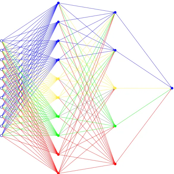
Figure 4gives and example of an MLP with 4 models. Here, the red model depends on green and yellow, which themselves depends on blue. Grey lines are the ones that can not be associated with an unique model (they can be associated with the (unordered) pair (𝑔𝑟𝑒𝑒𝑛, 𝑦𝑒𝑙𝑙𝑜𝑤)).
MLP will be our main test case for experiments. It will allow us to evaluate how our method works depending on various parameters.
IV.2 Associative neural network
We designed a custom kind of neural network using an associative learning rule. It is a proof of concept to show how our method performs on a network that differs significantly from MLP and use a learning algorithm different from gradient descent.
We took elements from Hopfield Network [Kv96] for the neurons themselves and Restricted Boltz-mann Machine [Smo86] for the structure of the network and the data is represented using Sparse Distributed Representation [AH15]. Our network is divided into a visible and a hidden layer, forming a complete (directed) bipartite graph. Activation function are fixed thresholds (output is either1 or
0). The network is used for completion tasks: a partial vector (with 0 instead of 1 for some of its coordinates) is given as input and the network must return the complete vector as output.
Figure 4: A multi-layer perceptron with 4 partial models
The process is the following: the visible layer’s neurons outputs are set to the values of the input vector, the hidden layers’ neuron’s output is computed from the values of the visible layer, finally, the visible neurons values are updated, based on the hidden layer’s values. The computation is simple: if the weighted sum of inputs is ⩾ some threshold (hyperparamter), the output is 1, 0 otherwise. See Algorithm 3for pseudo-code.
For learning, the network is given a complete vector as input, then the hidden layer’s values are computed, finally, both layer’s neuron’s weights are updated. The learning rule is the following : if two neurons are active together, the weight of the link between them is increased, if one is active and not the other, this weight is decreased. Increments values depends on a fixed learning rate and weights are limited to [−1; 1]. See Algorithm 4for pseudo-code.
V Experiments
Our experiments aim to show the efficiency of our method on simple examples and evaluate how this efficiency is affected by various parameters. While real world applications of our method are likely to be more complex, those simple examples are an efficient way to provide detailed results about our method’s behavior.
Algorithm 3:Computation
Data: 𝑡ℎ𝑙𝑑threshold for neurons’ activation
1 for 0 ⩽ 𝑖 < ℎ𝑖𝑑𝑑𝑒𝑛.𝑠𝑖𝑧𝑒 do 2 if𝑣𝑖𝑠𝑖𝑏𝑙𝑒.𝑜𝑢𝑡𝑝𝑢𝑡 ⋅ ℎ𝑖𝑑𝑑𝑒𝑛.𝑤𝑒𝑖𝑔ℎ𝑡[𝑖] ⩾ 𝑡ℎ𝑙𝑑 then 3 ℎ𝑖𝑑𝑑𝑒𝑛.𝑜𝑢𝑡𝑝𝑢𝑡[𝑖] ← 1 4 else 5 ℎ𝑖𝑑𝑑𝑒𝑛.𝑜𝑢𝑡𝑝𝑢𝑡[𝑖] ← 0 6 for 0 ⩽ 𝑖 < 𝑣𝑖𝑠𝑖𝑏𝑙𝑒.𝑠𝑖𝑧𝑒do 7 ifℎ𝑖𝑑𝑑𝑒𝑛.𝑜𝑢𝑡𝑝𝑢𝑡 ⋅ 𝑣𝑖𝑠𝑖𝑏𝑙𝑒.𝑤𝑒𝑖𝑔ℎ𝑡[𝑖] ⩾ 𝑡ℎ𝑙𝑑 then 8 𝑣𝑖𝑠𝑖𝑏𝑙𝑒.𝑜𝑢𝑡𝑝𝑢𝑡[𝑖] ← 1 9 else 10 𝑣𝑖𝑠𝑖𝑏𝑙𝑒.𝑜𝑢𝑡𝑝𝑢𝑡[𝑖] ← 0 V.1 Multi-Layer Perceptron
For our experiments with MLP, we used the well-known MNIST [LeC+98] data set. The task is simple: recognize handwritten digits. To generate different but related learning tasks for each peer, we permute digits. Our multi-layer perceptron was trained using classical Stochastic Gradient Descent with Back Propagation [RHW86].
We use the following notation to describe our MLPs’ layouts: 𝑛=𝑚=𝑝=𝑞 means that we have a four-layer MLP (including input and output, so, 2 hidden layers) with 𝑛 neurons on the first (input) layer,𝑚 on the second, and so on. We will use a similar notation to describe partial models: 𝑛-𝑚-𝑝-𝑞
means that the described model has 𝑛neurons for the first layer, 𝑚 for the second, and so on. We use a 784=300=100=10 configuration for our MLP (two hidden layers), unless explicitly stated otherwise, a fixed learning rate of 0.1 and a sigmoid activation function 𝑓(𝑥) = 1+𝑒1−𝑥.
The “Accuracy” metrics is simply the proportion of recognized digits. A digit is considered recog-nized if the most active neuron of the last layer corresponds to this digit.
To obtain different training sets for different peers, we divided the MNIST training set in successive sequences. This is important because practical implementations will be likely to have peers with completely independent data; keeping data local being one of the key features of our method. The test set is the 1000 first digits of the MNIST test set.
We performed a total of 9 independent tests with MLP, each designed to evaluate one specific aspect of our system: partial averaging efficiency, convergence, effect of the number of peers, semi-local models, semi-semi-local+semi-local models, effect of the level of difference between tasks, effect on the number of peers with modified tasks, effect of the training set size, use of a more problem-specific layout.
V.1.a Averaging level
This first experiment aims to show that performing a partial averaging is better, in the considered multi-task situation, than a complete averaging or no averaging and to determine which level of averaging is the best.
For this experiment we used 16 peers, each with a training set of 3500 digits. All the training sets are different, not overlapping, parts of the whole MNIST training set (60000 digits). These choices are a compromise to have a sufficient number of peers while not reducing the training set size too much and maintaining independent training sets, with MNIST training set size limitation.
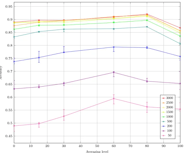
The “averaging level” is the number of neurons in the global model (shared by all peers), others neurons being in local models, in the second hidden layers, which contains a total of 100 neurons. The levels we tested are 0, 15, 30, 60, 80 and 100. Some neurons from the first hidden layer are also
Algorithm 4:Learning
Data: 𝑡ℎ𝑙𝑑threshold for neurons’ activation,𝑙 the learning rate
1 for 0 ⩽ 𝑖 < ℎ𝑖𝑑𝑑𝑒𝑛.𝑠𝑖𝑧𝑒 do 2 for0 ⩽ 𝑗 < 𝑣𝑖𝑠𝑖𝑏𝑙𝑒.𝑠𝑖𝑧𝑒 do 3 if𝑣𝑖𝑠𝑖𝑏𝑙𝑒.𝑜𝑢𝑡𝑝𝑢𝑡[𝑗] == 1 then 4 ifℎ𝑖𝑑𝑑𝑒𝑛.𝑜𝑢𝑡𝑝𝑢𝑡[𝑖] == 1 then 5 ℎ𝑖𝑑𝑑𝑒𝑛.𝑤𝑒𝑖𝑔ℎ𝑡[𝑖][𝑗]+ = 1−ℎ𝑖𝑑𝑑𝑒𝑛.𝑤𝑒𝑖𝑔ℎ𝑡[𝑖][𝑗]2 𝑙 6 else 7 ℎ𝑖𝑑𝑑𝑒𝑛.𝑤𝑒𝑖𝑔ℎ𝑡[𝑖][𝑗]− = 1+ℎ𝑖𝑑𝑑𝑒𝑛.𝑤𝑒𝑖𝑔ℎ𝑡[𝑖][𝑗]2 𝑙 8 for 0 ⩽ 𝑖 < 𝑣𝑖𝑠𝑖𝑏𝑙𝑒.𝑠𝑖𝑧𝑒do 9 for0 ⩽ 𝑗 < ℎ𝑖𝑑𝑑𝑒𝑛.𝑠𝑖𝑧𝑒do 10 ifℎ𝑖𝑑𝑑𝑒𝑛.𝑜𝑢𝑡𝑝𝑢𝑡[𝑗] == 1then 11 if𝑣𝑖𝑠𝑖𝑏𝑙𝑒.𝑜𝑢𝑡𝑝𝑢𝑡[𝑖] == 1 then 12 𝑣𝑖𝑠𝑖𝑏𝑙𝑒.𝑤𝑒𝑖𝑔ℎ𝑡[𝑖][𝑗]+ = 1−𝑣𝑖𝑠𝑖𝑏𝑙𝑒.𝑤𝑒𝑖𝑔ℎ𝑡[𝑖][𝑗]2 𝑙 13 else 14 𝑣𝑖𝑠𝑖𝑏𝑙𝑒.𝑤𝑒𝑖𝑔ℎ𝑡[𝑖][𝑗]− = 1+𝑣𝑖𝑠𝑖𝑏𝑙𝑒.𝑤𝑒𝑖𝑔ℎ𝑡[𝑖][𝑗]2 𝑙
averaged, the exact numbers are, respectively, 0, 50, 100, 200, 250, 300. Each line corresponds to a different mini-batch size (from 50 to 3000). The averaging process was done after every mini-batch. 30 mini-batches were used for training. Differences between peers are induced by inverting digits 8 and 9 for 7 of the 16 peers, giving us a close to but not even split.
Results are median of 10 runs. The error bars corresponds to the third and fifth quintiles. The results are presented in Figure5.
From those results, we can conclude that, whatever the mini-batch size is, the best performance is always achieved using partial averaging. For higher mini-batch size, the best performance is achieved with an averaging level of 80.
The significant drop of performance observed with an averaging level of 100 is due to fact that a unique model can not address the permutation of 8 and 9 for certain peers. This validates our partial averaging concept.
V.1.b Convergence
The point of this test is to see how the accuracy evolves during the training process.
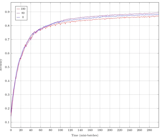
For this experiment we tested different averaging levels, with 16 peers, a fixed mini-batch size of 100. Training sets are independent and of size 3500. The smaller mini-batch size allows finer grain in accuracy sampling.
The “averaging level” is the number of neurons in the global model (shared by all peers), others neurons being in local models, in the second hidden layers, which contains a total of 100 neurons. The levels we tested are 0, 80 and 100. Some neurons from the first hidden layer are also averaged, the exact numbers are, respectively, 0, 250, 300. Each line corresponds to a different averaging level. The averaging process was done every 10 mini-batch. 30 mini-batches were used for training. Differences between peers are induced by inverting digits 8 and 9 for 7 of the 16 peers.
Results are median of 10 runs. The results are presented in Figure 6.
At the beginning of the training, no averaging is leading and 80 averaging is last but when ap-proaching maximum accuracy, 80 becomes first and 100 last. The three curves have similar shapes and remain very close.
0 10 20 30 40 50 60 70 80 90 100 0.45 0.5 0.55 0.6 0.65 0.7 0.75 0.8 0.85 0.9 0.95 Averaging level A ccuracy
Accuracy depending on averaging level and mini-batch size
3000 2500 2000 1500 1000 500 200 100 50
Figure 5: Accuracy for various averaging levels and mini-batch sizes V.1.c Number of peers
In this experiment, we want to evaluate how different averaging levels’ performances are affected by the number of peers.
For this experiment we tested different numbers of peers, from 4 to 16, and different averaging levels with a fixed mini-batch size of 500. Training sets are independent and of size 3500.
The “averaging level” is the number of neurons in the global model (shared by all peers), others neurons being in local models, in the second hidden layers, which contains a total of 100 neurons. The levels we tested are 0, 15, 30, 60, 80 and 100. Some neurons from the first hidden layer are also averaged, the exact numbers are, respectively, 0, 50, 100, 200, 250, 300. Each line corresponds to a different averaging level. The averaging process was done after every mini-batch. 30 mini-batches were used for training. Differences between peers are induced by inverting digits 8 and 9 for one fourth of peers. This ration diving evenly all tested numbers of peers.
Results are median of 10 runs. The error bars corresponds to the third and fifth quintiles. The results are presented in Figure7.
We see here that, obviously, the number of peers has no effect when averaging is not used. It also has a small effect with a limited averaging level but, with high level partial averaging (60-80), we get a significant performance gain when increasing the number of peers. The performance of full averaging, despite gaining from peer number increase, remains low. This indicates that partial averaging allows for performance gain when connecting more peers, giving access to more training examples.
0 20 40 60 80 100 120 140 160 180 200 220 240 260 280 0.1 0.2 0.3 0.4 0.5 0.6 0.7 0.8 0.9 Time (mini-batches) A ccuracy
Accuracy variation over time (convergence) for various averaging levels
100 80
0
Figure 6: Accuracy over time (convergence) for various averaging levels V.1.d Semi-local averaging
Here, we want to see how semi-local models can improve performance, compared to just using global and local models.
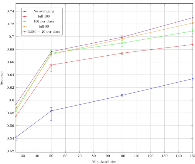
For this experiment we tested different averaging schemes with different mini-batch sizes (from 25 to 150). Smaller mini-batches allowing more frequent averaging for this more difficult context. Training sets are independent and of size 200, so that the smaller mini-batches would still cover a significant portion of the training sets. We used 12 peers; a highly divisible number allowing more complex permutation patterns.
The schemes tested are the following: no averaging, complete averaging of all peers’ neural net-works, complete averaging limited to peers with identical permutation, averaging with a 80 level of all peers’ neural networks, averaging with a 80 level of all peers’ neural networks + averaging with a 20 level of peers with identical permutation. Each line corresponds to a different averaging scheme. The averaging process was done after every mini-batch. 100 mini-batches were used for training. Differ-ences between peers are induced by applying all elements of𝔖3 to the last 3 digits. Each permutation is used for 2 peers (12 peers total).
Results are median of 20 runs (more precise than 10, since results were close). The error bars corresponds to the third and fifth quintiles. The results are presented in Figure8.
On this test, we observe that no averaging is the method with the worst performance. Full averaging is better but still less efficient than averaging per class or 80 averaging. Having a 800 global model +
4 5 6 7 8 9 10 11 12 13 14 15 16 0.81 0.82 0.83 0.84 0.85 0.86 0.87 0.88 Number of peers A ccuracy
Accuracy depending on number of peers and averaging level 100 80 60 30 15 0
Figure 7: Accuracy for various numbers of peers and averaging levels a 20 semi-local model ended-up begin the best solution here.
V.1.e Semi-local averaging with local models
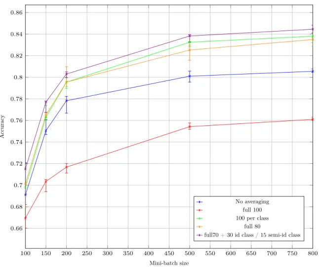
In this test, we evaluate how a combination of global, semi-local and locals models performs. For this experiment we tested different averaging schemes with different mini-batch sizes (from 100 to 800), allowing a medium averaging frequency, adapted to the difficulty of the task (complex permutation set, but with few peers). Training sets are independent and of size 1000. We used 4 peers, less peers implying that some would have unique permutations, the natural use-case for local models.
The schemes tested are the following: no averaging, complete averaging of all peers’ neural net-works, complete averaging limited to peers with identical permutation, averaging with a 80 level of all peers’ neural networks, averaging with a 70 level (784-220-70-10) of all peers’ neural networks + averaging with a 30 level (0-80-30-0) for peers 0 and 1 and an averaging with a 15 level (0-40-15-0) for peers 2 and 3. Each line corresponds to a different averaging scheme. The averaging process was done after every mini-batch. 50 mini-batches were used for training. Differences between peers are induced by inverting digits 8 and 9 for peer 2 and 3 + digits 6 and 7 for peer 3.
Results are median of 20 runs (more precise than 10, since results were close). The error bars corresponds to the third and fifth quintiles. The results are presented in Figure9.
30 40 50 60 70 80 90 100 110 120 130 140 150 0.52 0.54 0.56 0.58 0.6 0.62 0.64 0.66 0.68 0.7 0.72 0.74 Mini-batch size A ccuracy
Accuracy depending on mini-batch size and averaging scheme No averaging
full 100 100 per class
full 80 full80 + 20 per class
Figure 8: Accuracy for various mini-batch sizes and averaging schemes
all other schemes, including no averaging. 80 averaging was better than no averaging, but still inferior to 100 averaging per class with big enough mini-batches. 70 + 30 for identical peers and 15 for peers with only one common inversion was the best.
V.1.f Difference rate
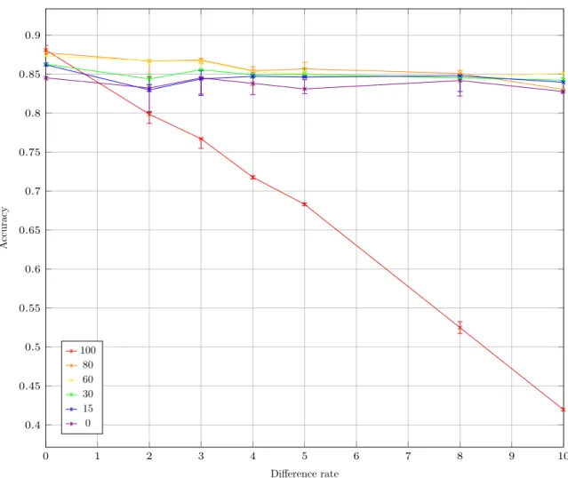
Here we want to see how the efficiency of different averaging level is affected by the level of difference between peers’ tasks.
We tested different averaging levels for different difference rates. The difference rate being the number of digits affected by a different permutation between peers, ranging from 0 to 10. Training sets are independent and of size 3500; mini-batch size is 500. We used 16 peers. Each line corresponds to a different averaging level. The averaging process was done after every mini-batch. 30 mini-batches were used for training. Differences between peers are induced by applying the cycle(10 − 𝑟…9)where
𝑟 is the difference rate (or no permutation if 𝑟 = 0,𝑟 = 1 being impossible with this system) to 7 of the 16 peers output.
Results are median of 10 runs. The error bars corresponds to the third and fifth quintiles. The results are presented in Figure10.
We observe that, while it seems to be the best when there is no difference (the gap with 80 and 60 is to low to officially conclude), 100 averaging is the only scheme severely affected by the difference rate, loosing more than 50% of accuracy. For other schemes, 80 and 60 are the best for low difference
100 150 200 250 300 350 400 450 500 550 600 650 700 750 800 0.66 0.68 0.7 0.72 0.74 0.76 0.78 0.8 0.82 0.84 0.86 Mini-batch size A ccuracy
Accuracy depending on mini-batch size and averaging scheme
No averaging full 100 100 per class
full 80
full70 + 30 id class / 15 semi-id class
Figure 9: Accuracy for various mini-batch sizes and averaging schemes
rate but the gap is significantly reduced when the difference rate increases. For 10, 80 seems to be inferior to other partial averaging scheme, with a level of accuracy similar to no averaging.
V.1.g Number of peers with permutation
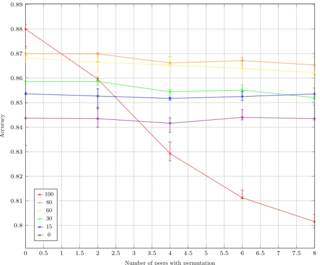
Here we want to see how the efficiency of different averaging level is affected by the proportion of peers with a non-trivial permutation.
We tested different averaging levels for number of peers with permutation. Training sets are independent and of size 3500; mini-batch size is 500. We used 16 peers. Each line corresponds to a different averaging level. The averaging process was done after every mini-batch. 30 mini-batches were used for training. The peers with a non-trivial permutation have 8 and 9 permuted.
Results are median of 20 runs (more precise than 10, since results were close). The error bars corresponds to the third and fifth quintiles. The results are presented in Figure11.
We observe that full averaging’s accuracy significantly drops when the number of permuted peers increases. Full averaging is the most accurate with 0 peers with permutations (logical) but is only third with 2 and last for 4 to 8. As one could expect, no averaging is not affected by the number of peers with permutation. More interestingly, partial averaging schemes do not seem to be much affected by the number of peers with permutation; only a limited drop is observed for 30, 60 and 80.
0 1 2 3 4 5 6 7 8 9 10 0.4 0.45 0.5 0.55 0.6 0.65 0.7 0.75 0.8 0.85 0.9 Difference rate A ccuracy
Accuracy depending on difference rate and averaging level
100 80 60 30 15 0
Figure 10: Accuracy for various difference rates and averaging levels V.1.h Training set size
Here we want to see how the efficiency of different averaging level is affected by the size of each peer’s training set.
We tested different averaging levels for different training set sizes (ranging from 250 to 3500). The mini-batch size is fixed at 200. We used 16 peers. Each line corresponds to a different averaging level. The averaging process was done after every mini-batch. 50 mini-batches were used for training. Differences between peers are induced by inverting digits 8 and 9 for 7 of the 16 peers.
Results are median of 10 runs. The error bars corresponds to the third and fifth quintiles. The results are presented in Figure12.
We see that the lower the averaging level is, the more the training set size is important. 100 averaging is the best for 250 set size, third behind 80 and 60 for 500, bets only 0 for 1000 and last after that. 80 is the best averaging level, except for very small training sets (size 250); 60 being second. V.1.i A different layout
Due to the way we induce differences between peers, a simple post-treatment consisting in a permutation inversion would allow 100 averaging to outperform any scheme. We did not tried to use this fact before to improve our averaging schemes to remain general. In this test, we evaluate how a partial averaging scheme crafted more specifically for this problem will perform.
0 0.5 1 1.5 2 2.5 3 3.5 4 4.5 5 5.5 6 6.5 7 7.5 8 0.8 0.81 0.82 0.83 0.84 0.85 0.86 0.87 0.88 0.89
Number of peers with permutation
A
ccuracy
Accuracy depending on number of peers with permutation and averaging level
100 80 60 30 15 0
Figure 11: Accuracy for various numbers of peers with permutation and averaging levels schemes are used with a 784=300=100=10 network layout (4 layers), last 4 784=300=100=10=10 (5 layers). Each line corresponds to a different averaging scheme. Training sets are independent and of size 3500; mini-batch size is 500. We used 16 peers. The averaging process was done after every mini-batch. 50 mini-batches were used for training (longer training, since some layouts are deeper than usual). Differences between peers are induced by applying the cycle (10 − 𝑟…9) where 𝑟 is the difference rate (or no permutation if 𝑟 = 0, 𝑟 = 1 being impossible with this system) to 7 of the 16 peers output.
Results are median of 10 runs. The error bars corresponds to the third and fifth quintiles. The results are presented in Figure13.
Like previously, complete averaging schemes see their accuracy drop severely when the difference rate increases. The 80 variant used on 784=300=100=10=10 has an accuracy close to no averaging on the same layout, lower for high difference rates. 784=300=100=10=10 layout seems less efficient than 784=300=100=10 in general, but with a 784-300-100-10-0 averaging scheme, it outperforms no averaging on 784=300=100=10 and even (but not much significantly) 784-250-80-10 for high difference rates. 784-300-100-0 appears to be the best scheme in general, beating any other scheme significantly, except in the no difference case and being less affected than 784-250-80-10 by difference rate.
It is important to remember that the 784-300-100-0 was the best here due to the particular nature of the differences between peers, a permutation. This scheme was crafted specifically for this problem, which is a luxury, we could not have done this if the exact nature of the differences between peers was
400 600 800 1,000 1,200 1,400 1,600 1,800 2,000 2,200 2,400 2,600 2,800 3,000 3,200 3,400 0.64 0.66 0.68 0.7 0.72 0.74 0.76 0.78 0.8 0.82 0.84 0.86
Training sets size
A
ccuracy
Accuracy depending on training sets size and averaging level 100 80 60 30 15 0
Figure 12: Accuracy for various training sets sizes and averaging levels
not precisely known. Moreover, this kind of layout is not easy to generalize to semi-local models.
V.2 Associative neural network
We did our tests with associative neural network on the following task.
We generate binary vectors of size𝑛(∈ 0, 1𝑛) with2𝑚 1s (and𝑛 − 2𝑚 0s). The task of the neural
network is to be able to complete each learned vector from an input with only𝑚 1s. For example, the learned vector could be [0, 0, 1, 0, 1, 1, 0, 0, 1], the neural network will be given [0, 0, 1, 0, 0, 1, 0, 0, 0]as input and should be able to return the learned vector.
For training, the network is given the full vectors as input then, for testing, we give the network a partial input with only 𝑚 1s and observe the output. To complicate the task, we add noise to the vectors: a fixed number𝑧of random coordinates are inverted in all vector (training and testing) before feeding them to the network.
For accuracy evaluation, the task is considered successfully accomplished the number of matching
1s between expected output and actual output is greater than (or equal to) the number of non-matching one1, more formally (c is expected output,a is actual output), a test is considered successful if and only if c∧a as more or as many 1s thanc⊕a.
To generate difference between peers, we simply changed for some peers the half of the 1s that are not in the testing input. For example, from [0, 0, 1, 0, 0, 1, 0, 0, 0], some peers will have to find
0 1 2 3 4 5 6 7 8 9 10 0.4 0.45 0.5 0.55 0.6 0.65 0.7 0.75 0.8 0.85 0.9 Difference rate A ccuracy
Accuracy depending on difference rate and layout-scheme
0-0-0-0 784-250-80-10 784-300-100-10 784-300-100-0 784-300-100-10-0 0-0-0-0-0 784-250-80-8-10 784-300-100-10-10
Figure 13: Accuracy for various difference rates and layouts-schemes
Our vector generator work the following way: it takes as input an integral 𝑘 ∈ ℕ and has a parameter𝑠 which is periodicity of the generator. The1 of the vector that will be given as input for both training and testing corresponds to the coordinates3𝑚(𝑘[𝑠]) + 𝑖 with𝑖ranging from0to𝑚 − 1. The 1 of the vector that will be given as input only for training (that should be guessed for testing) corresponds to the coordinates3𝑚(𝑘[𝑠]) + 𝑖with𝑖ranging from𝑚 to2𝑚 − 1 in the general case and, in the modified case (when we want to make a peer different), with 𝑖 ranging from 2𝑚 to 3𝑚 − 1.
To add noise, we simply flip bits with coordinates ((𝑘/𝑠) + 𝑖(𝑛/𝑧))[𝑛] (/ is integral quotient) with 𝑖
ranging from 0to𝑧 − 1.
For this test, we used 15 peers, 2 of them having 1 out of 3 vectors modified. The vectors were 50 bits long, with 𝑚 = 8 (non-zero bits) and𝑧 = 2 (noise). The generators periodicity was 3, the batch size was 9 (𝑘 ∈〚0, 9〚) and the mini-batch size was 3. The tests were done for100 consecutive values of 𝑘(starting at1000). The learning rate was0.1. The threshold for neurons activation was0.5. The
visible layer had 50 neurons (the length of an input/output vector), the hidden layer had 400 neurons. We tested with no averaging at all, complete averaging of both layers (visible and hidden) and several partial averaging schemes. For partial averaging schemes, the visible layer was completely averaged and 100, 200, 300 or 350 neurons of the hidden layer were averaged. Each line corresponds to a particular number of mini-batches used: 10, 20, 30 or 40. Averaging was done after each mini-batch. Results are median of 100 runs. The error bars corresponds to the third and fifth quintiles. The results are presented in Figure14.
0 50 100 150 200 250 300 350 400 0.4 0.45 0.5 0.55 0.6 0.65 0.7 0.75 0.8 0.85 0.9 0.95 1 Averaging level A ccuracy
Accuracy depending on averaging level and mini-batches number
40 30 20 10
Figure 14: Accuracy for various averaging levels and mini-batches number
We observe here that an averaging level of 300 (over 400) seems optimal for lower numbers of mini-batches (10,20), while 350 is for higher numbers (30,40). Except for 40 mini-mini-batches, partial averaging schemes are always the best. Complete averaging was the worst for all tests but the 40 mini-batches one. For 40 mini-batches, complete averaging, while still worse than partial 350, is better than most partial averaging schemes. For all numbers of mini-batches, the optimal averaging level remained around 300-350.
V.3 General analysis of results
Tests recapitulation(“Classic” is 784=300=100=10)
Task [NN] Peers Batch size MB size MB number Avg every Layout Averaging Difference [#peers]
MNIST [MLP] 16 3500 Varies 30 1 Classic Varies (89) [7]
MNIST [MLP] 16 3500 100 30 10 Classic Varies (89) [7]
MNIST [MLP] Varies 3500 500 30 1 Classic Varies (89) [1/4]
MNIST [MLP] 12 200 Varies 100 1 Classic Varies 𝔖3[2 each]
MNIST [MLP] 4 1000 Varies 50 1 Classic Varies (89) [1] + (67)(89) [1]
MNIST [MLP] 16 3500 500 30 1 Classic Varies Varies [7]
MNIST [MLP] 16 3500 500 30 1 Classic Varies (89) [Varies]
MNIST [MLP] 16 Varies 200 50 1 Classic Varies (89) [7]
MNIST [MLP] 16 3500 500 50 1 Varies Varies Varies [7]
SBV compl [Assoc] 15 9 3 Varies 1 50<>400 Varies Half 1s [2]
After those tests, we can state that our method effectively enables multi-task learning with neural networks. From the presented results, we can make the following detailed statements.
Partial model averaging have proved its capacity to obtain better results than no averaging or complete averaging on different tasks with a variety of parameters, different kinds of neural networks and learning algorithms. Among tasks tested, a high level of averaging (60-80%) was usually the best solution and the level of difference between peers’ tasks only has a low influence on the optimal averaging level. Semi-local averaging, while only allowing a limited gain, has proved its efficiency on cases where groups of peers share more similar functions than the whole system. More task-specific layouts, averaging limited to task-specific layers, have proved to be more efficient in the case digit permutation but require more knowledge about the differences between peers and may not (easily) allow semi-local models.
While those tests are done on simple cases: MNIST and sparse binary vector completion, they allowed us to examine numerous parameters changes and their effect on the efficiency of our method. This makes this paper a good base for applying our work to real use cases.
VI Related work
A number of researchers have addressed the problem of distributed [Rec+11;Smi+16], decentral-ized [Bel+18] or federated learning [Kon+16] while focusing on single tasks. Most of these works con-sider (Stochastic) Gradient Descent, even if some approaches, like federated model averaging [Bre+17], can in principle be applied to other learning algorithms. In the context of model averaging, a recent contribution [Kam+19] suggests that changing the frequency of (model) synchronization depending on the obtained accuracy can reduce communication overhead. We plan to consider this possibility as future work.
The majority of solutions for multi-task learning focus on a local setup, rather than a distributed one [Rud17], but some decentralized solutions exist. The first, to the best of our knowledge, such contribution [OHJ12] proposes a decentralized multi-task learning algorithm limited to linear models, a work later improved in [WKS16] and [Smi+17]. A recent theoretical paper [CST18] proposes the use of kernel methods to learn non-linear models in federated learning. Some researchers have instead proposed a form of decentralized multi-task learning, in which each peer needs to learn a personalized convex model influenced by neighborhood relationships in a collaboration graph [Bel+18]. In a more recent paper, they also presented an algorithm to jointly learn both the personalized convex models and the collaboration graph itself [ZBT19]. In this paper, we do not use a collaboration graph; rather, we express similarities between learning tasks by defining sub-models that are shared with the entire networks (global models) or with group of peers (semi-local models). Moreover unlike the above solutions, our approach can optimize non-convex loss functions.
Finally, a very recent preprint [CB19] proposes a method for federated multi-task learning with neural networks. However, this proposal relies on a client-server model in which clients operate in a sequential fashion, performing their updates one after the other. This negates any speed gains that may result from distribution and results in very poor scalability making this method unsuitable for most practical applications.
VII Conclusion
In this work, we introduced an effective solution for distributed multi-task learning with neural networks, applicable with different kinds of learning algorithms and not requiring mandatory prior knowledge about the nature, nor magnitude, of the differences between tasks, while still being able to benefit from such knowledge when available. The simplicity, range of application and flexibility of our method significantly distinguishes it from existing works.
This work could be continued in the following directions. Developing an algorithm that allow models to be automatically assigned to peers. Trying to reduce communication overhead in a way
similar to [Kam+19]. Figuring out what a good peer sampling algorithm to use with our method in a distributed context would be. Trying our method with more kinds of neural networks, like LSTM [HS97]. Examining the question of the individual gains for peers, their differences and the consequences it may have if peers are considered as rational economic agents.
References
[AH15] Subutai Ahmad and Jeff Hawkins. “Properties of Sparse Distributed Representations and their Application to Hierarchical Temporal Memory”. In: CoRR(2015).
[Bel+18] Aurélien Bellet et al. “Personalized and Private Peer-to-Peer Machine Learning”. In: Pro-ceedings of the Twenty-First International Conference on Artificial Intelligence and Statis-tics. Ed. by Amos Storkey and Fernando Perez-Cruz. Vol. 84. Proceedings of Machine Learning Research. PMLR, 2018, pp. 473–481.
[BFT19] Amaury Bouchra Pilet, Davide Frey, and François Taïani. “Robust Privacy-Preserving Gossip Averaging”. In: Stabilization, Safety, and Security of Distributed Systems. Ed. by Mohsen Ghaffari et al. Vol. 11914. Lecture Notes in Computer Science. Springer Interna-tional Publishing, 2019, pp. 38–52.
[Bre+17] Hugh Brendan McMahan et al. “Communication-Efficient Learning of Deep Networks from Decentralized Data”. In: Proceedings of the 20th International Conference on Artificial Intelligence and Statistics. Ed. by Aarti Singh and Jerry Zhu. Vol. 54. Proceedings of Machine Learning Research. PMLR, 2017, pp. 1273–1282.
[CB19] Luca Corinzia and Joachim M. Buhmann. “Variational Federated Multi-Task Learning”. 2019.
[Che+17] Min Chen et al. “Disease Prediction by Machine Learning Over Big Data From Healthcare Communities”. In: IEEE Access 5 (2017), pp. 8869–8879.
[CST18] Sebastian Caldas, Virginia Smith, and Ameet Talwalkar. “Federated Kernelized Multi-Task Learning”. In: SysML Conference 2018. 2018.
[GBC16] Ian Goodfellow, Yoshua Bengio, and Aaron Courville. Deep Learning. MIT Press, 2016. [HS97] Sepp Hochreiter and Jürgen Schmidhuber. “Long Short-Term Memory”. In: Neural
Com-putation 9.8 (1997), pp. 1735–1780.
[JMB05] Márk Jelasity, Alberto Montresor, and Ozalp Babaoglu. “Gossip-Based Aggregation in Large Dynamic Networks”. In: ACM Transactions on Computer Systems 23.3 (2005), pp. 219–252.
[Kam+19] Michael Kamp et al. “Efficient Decentralized Deep Learning by Dynamic Model Aver-aging”. In: Machine Learning and Knowledge Discovery in Databases. Ed. by Francesco Bonchi Michele Berlingerio and et al. Springer International Publishing, 2019, pp. 393– 409.
[Kon+16] Jakub Konečný et al. “Federated Optimization: Distributed Machine Learning for On-Device Intelligence”. 2016.
[Kv96] Ben Kröse and Patrick van der Smagt.An introduction to Neural Networks. 8th ed. 1996. [LB95] Yann LeCun and Yoshua Bengio. “Convolutional networks for images, speech, and time-series”. In:The handbook of brain theory and neural networks. Ed. by M.A. Arbib. Vol. 1. MIT Press, 1995, pp. 255–258.
[LeC+98] Yann LeCun et al. “Gradient-based learning applied to document recognition”. In: Pro-ceedings of the IEEE 86.11 (1998), pp. 2278–2324.
[OHJ12] Róbert Ormándi, István Hegedűs, and Márk Jelasity. “Gossip learning with linear models on fully distributed data”. In: Concurrency and Computation: Practice and Experience 25.4 (2012), pp. 556–571.
[Rec+11] Benjamin Recht et al. “Hogwild: A Lock-Free Approach to Parallelizing Stochastic Gra-dient Descent”. In: Advances in Neural Information Processing Systems 24. Ed. by J. Shawe-Taylor et al. Curran Associates, Inc., 2011, pp. 693–701.
[RHW86] David E. Rumelhart, Geoffrey E. Hinton, and Ronald J. Williams. “Learning Internal Representations by Error Propagation”. In: Parallel Distributed Processing: Explorations in the Microstructure of Cognition. Ed. by David E. Rumelhart, James L. McClelland, and PDP Research Group, CORPORATE. Vol. 1. MIT Press, 1986, pp. 318–362.
[Rud17] Sebastian Ruder. “An Overview of Multi-Task Learning in Deep Neural Networks”. 2017. [Shi+16] Weisong Shi et al. “Edge Computing: Vision and Challenges”. In:IEEE Internet of Things
Journal 3.5 (2016), pp. 637–646.
[Smi+16] Virginia Smith et al. “CoCoA: A General Framework for Communication-Efficient Dis-tributed Optimization”. In: Journal of Machine Learning Research 18 (2016).
[Smi+17] Virginia Smith et al. “Federated Multi-Task Learning”. In:Advances in Neural Information Processing Systems 30. Ed. by I. Guyon et al. Curran Associates, Inc., 2017, pp. 4424– 4434.
[Smo86] Paul Smolensky. “Information Processing in Dynamical Systems: Foundations of Harmony Theory”. In: Parallel Distributed Processing: Explorations in the Microstructure of Cog-nition. Ed. by David E. Rumelhart, James L. McClelland, and PDP Research Group, CORPORATE. Vol. 1. MIT Press, 1986, pp. 194–281.
[WKS16] Jialei Wang, Mladen Kolar, and Nathan Srerbo. “Distributed Multi-Task Learning”. In: Proceedings of the 19th International Conference on Artificial Intelligence and Statistics. Ed. by Arthur Gretton and Christian C. Robert. Vol. 51. Proceedings of Machine Learning Research. PMLR, 2016, pp. 751–760.
[ZBT19] Valentina Zantedeschi, Aurélien Bellet, and Marc Tommasi. “Fully Decentralized Joint Learning of Personalized Models and Collaboration Graphs”. 2019.