A Distributionally Robust Optimization Approach for the Optimal Wind Farm Allocation in Multi-Area Power Systems

A DISTRIBUTIONALLY ROBUST OPTIMIZATION APPROACH FOR THE OPTIMAL WIND FARM ALLOCATION IN MULTI-AREA POWER SYSTEMS

A Dissertation by

FAHAD SALEH M ALISMAIL

Submitted to the Office of Graduate and Professional Studies of Texas A&M University

in partial fulfillment of the requirements for the degree of DOCTOR OF PHILOSOPHY

Chair of Committee, Chanan Singh Committee Members, Mehrdad Ehsani

Laszlo Kish Lewis Ntaimo Head of Department, Miroslav Begovic

December 2016

Major Subject: Electrical Engineering

ABSTRACT

This dissertation presents a distributionally robust planning model to determine the optimal allocation of wind farms in a multi-area power system, so that the ex-pected energy not served (EENS) is minimized under uncertain conditions of wind power and generator forced outages. Unlike conventional stochastic programming approaches that rely on detailed information of the exact probability distribution, this proposed method attempts to minimize the expectation term over a collection of distributions characterized by accessible statistical measures, so it is more practical in cases where the detailed distribution data is unavailable. This planning model is for-mulated as a two-stage problem, where the wind power capacity allocation decisions are determined in the first stage, before the observation of uncertainty outcomes, and operation decisions are made in the second stage under specific uncertainty re-alizations.

In this dissertation, the second-stage decisions are approximated by linear decision rule functions, so that the distributionally robust model can be reformulated into a tractable second-order cone programming problem. Case studies based on a five-area system are conducted to demonstrate the effectiveness of the proposed method. The model is extended to deal with the hybrid system by including the solar power as a third source of uncertainty besides the wind power and conventional generation forced outages. The correlation between the wind and solar power is investigated to capture the diversity and the availability of all included power resources.

Capacity credit is calculated to measure the effective load carrying capacity of the allocated renewable resources. The probabilistic method including Monte Carlo simulation is used to calculate the loss of load expectation (LOLE) at different peak

loads and analytically determined the capacity credit of wind and solar power genera-tion for several installed wind capacities. The penetragenera-tion factor and the availability of the renewable power generation are major factors influencing the capacity credit value, besides the overall power system reliability level.

The results reflect the usefulness of utilizing the distributionally robust optimiza-tion approach in the data-driven decision making. It positively responds with the amount of the information provided regarding the uncertain variables in the renew-able power generation allocation problem and sequentially in the system reliability and the yielded capacity credit values of the allocated renewable generation units.

DEDICATION

To the loving memory of my beloved father, Saleh Mohammad Alismail, who Almighty Allah has chosen to be next to Him, who brought me up in the best ways. His wise teachings, warm feelings and continuous support were very influential on my personality and success. He encouraged me to seek knowledge, and I hope that in future I would be exactly as he dreamed.

My beloved mother, "Um-Fahad", for her love, and constant encouragement who always worried about my studies and my life conditions. Your prayers and moral support will always boot my progress.

My wife, Fatimah, without whose love, endurance, constant support, patience, care and understanding I could never have made it through these studies. Thanks for your strong emotional support which make my life pleasant and more meaningful even in the hardest times.

My beautiful children, Iqbal, Saleh and Tareq. You always inspire me and have made me stronger and more fulfilled than I could have ever thought.

My brother Mohammad and my sisters Munerah, Nourah, Dalal, Shimaa, Aseel, Seba and Hissah. I am always grateful to you for your kind care and your interest in my success. You deserve my warm thanks for your encouragements and love.

ACKNOWLEDGEMENTS

I would like to convey my profound thanks and appreciation to my advisor, Pro-fessor Chanan Singh, whose experience, knowledge and persistence provide me a valuable assistance to accomplish my dissertation. I appreciate his patience and endurance. Professor Singh supported me throughout my coursework, built my con-fidence, encouraged me to a challenging dissertation topic, and guided me technically with his experience.

I would also like to thank my committee members Professor Mehrdad Ehsani, Professor Laszlo Kish and Professor Lewis Ntaimo for their guidance, constructive and positive feedback.

Very special thanks are due to Dr. Peng Xiong, for his eloquent, total support and invaluable advising.

NOMENCLATURE

System Indices i Indices of areas

j Indices of areas

l Indices of generation capacity levels or wind power levels s Indices of wind distribution types, e.g. seasons, day or night t Indices of load segments

System Sets F Set of all transmission lines

I Set of all areas for wind farms

J_if Set of areas receiving power from area iby tie lines Jt

i Set of areas delivering power to area i by tie lines

Lα Set of all wind power levels

Lγ Set of all levels of the generation in one area

Lδ _{Set of all levels of the total generation}

S Set of all wind distribution types T Set of all load segments

Notations for Uncertain Wind Power Generation ˜

w_is Random wind power generation as a percentage of the installed capacity, in area i under distribution type s. The vector of all ˜ws_i is denoted by ˜www, and a specific realization of ˜www is denoted bywww

¯

w_is The mean value of random wind power in area i under wind power distribution type s (p.u.)

W Uncertainty set of uncertain wind power ˜www Ws

il The selected level l of random wind power output ˜wsi (p.u.)

αs

il Absolute deviation of ˜wsi around the selected level Wils (p.u.)

β_ijs Mean absolute deviation of the summation of ˜ws_i and ˜ws_j (p.u.) λs_i The variance of random wind power ˜ws_i (p.u.)

Notations for Uncertain Generation Capacity ˜

pi Random generation capacity in area i. The vector of all ˜pi is denoted by ˜ppp,

and a specific realization of ˜pppis denoted byppp (MW) ¯

pi The mean value of the uncertain generation capacity in area i (MW)

pmax_i Upper bound of ˜pi (MW)

pmin_i Lower bound of ˜pi (MW)

P Uncertainty set of random generation capacity ˜ppp

Pil The selected generation level l of random generation capacity ˜pi (MW)

Ql The selected generation level l of the total generation capacity P i∈I˜

pi (MW)

γil The expected value of the positive part of Pil−p˜it (MW)

δl The expected value of the positive part of Ql− P i∈I ˜

pi (MW)

System Constants Ds

it The tth segment of load in area i under wind pattern types (MW)

Fij Capacity of tie line between areasi and j (MW)

Ts

t The duration of thetth segment of load under wind pattern type s (hours)

Πi The maximum wind capacity that can be installed in area i (MW)

Decision Variables

f_ijts Power flow from areai to areaj for demand segment t under wind distributions (MW)

qs_it Generation for demand segmentt in areai under wind distributions (MW) l_its Load loss for demand segmentt in area i under wind distributions (MW) xi Wind power capacity installed in areai (MW)

Indices for the Mathematical Formulation

k Indices of all functions characterizing the distributions of random variables, it is equivalent to the indices of auxiliary variables ˜uuu

m Indices of all first-stage and second-stage constraints n Indices of all first-stage and second-stage decision variables r Indices of all constraints that define the extended support set ¯Z v Indices of all random variables ˜zzz

Sets for the Mathematical Formulation

F Ambiguity set defining the distributions of all random variables

¯

F Extended ambiguity set

K Set of all functions characterizing the distributions of random variables, equivalent to the sets of auxiliary variables ˜uuu

M1 Set of all first-stage constraints

M2 Set of all second-stage constraints

N1 Set of all first-stage decision variables

N2 Set of all second-stage decision variables

R Set of all constraints that define the extended support set ¯Z V Set of all random variables ˜zzz

Z Uncertainty set of random variables ˜zzz ¯

Matrices and Vectors of the Mathematical Formulation AAA Matrix of the coefficients ofxxxfor first-stage constraints

bbb Right-hand-side vector of the first-stage constraints C

CC(zzz) Uncertain left-hand-side matrix of coefficient ofxxx for the second-stage constraints

DDD Left-hand-side matrix of coefficient ofyyy for the second-stage constraints d

dd(zzz) Uncertain right-hand-side vector of the second-stage constraints H

HH Matrix of the coefficients ofuuufor the constraints defining the extended support set ¯Z

h

hh Right-hand-side vector of the constraints defining extended support set ¯Z u

uu Auxiliary variables introduced into the extended ambiguity set ¯_F x

xx Vector of first-stage decision variables

yyy Vector of second-stage decision variables or decision rules zzz Vector of random variables

Others

EP Expected value under distribution P

gk(·) Linear representable functions characterizing the distributions of random

variableszzz

L(·) Function indicating energy not served

P A distribution of all random variableszzz

Q A distribution of all random variableszzz and auxiliary variablesuuu

Q0(·) Set of all distributions for random variables with the given dimension

TABLE OF CONTENTS Page ABSTRACT . . . ii DEDICATION . . . iv ACKNOWLEDGEMENTS . . . v NOMENCLATURE . . . vi

TABLE OF CONTENTS . . . xiii

LIST OF FIGURES . . . xvi

LIST OF TABLES . . . xviii

1. INTRODUCTION . . . 1

1.1 Wind Power Generation . . . 1

1.2 Probabilistic Modeling of Uncertainty . . . 2

1.3 Optimization Model under Uncertainty . . . 3

1.4 Distributionally Robust Optimization . . . 4

1.5 Monte Carlo Simulation for Generation Adequacy Evaluation . . . 5

1.6 Multi-Area Power System . . . 7

1.7 Organization of the Dissertation . . . 9

2. WIND FARM ALLOCATION PLANNING PROBLEM . . . 10

2.1 Linear Representation Formulation of Wind Power Statistical Param-eters . . . 10

2.1.1 A Two-Stage Wind Farm Allocation Model . . . 10

2.1.2 Ambiguity Set . . . 12

2.2 Problem Solving Procedure . . . 17

2.2.1 Compact Matrix Formulation . . . 17

2.2.2 Extended Ambiguity Set . . . 20

2.2.3 Reformulation with the Generalized Linear Decision Rule . . . 21

3. NONLINEAR FORMULATION OF WIND FARM ALLOCATION

PLAN-NING PROBLEM . . . 31

3.1 Nonlinear Representation of Wind Power Statistical Parameters . . . 31

3.1.1 A Two-Stage Wind Farm Allocation Model . . . 31

3.1.2 Ambiguity Set . . . 32

3.2 Problem Reformulation . . . 34

3.2.1 Compact Matrix Formulation . . . 34

3.2.2 Extended Ambiguity Set . . . 36

3.2.3 Reformulation with the Generalized Linear Decision Rule . . . 38

3.3 Case Studies on DRO Based Wind Power Generation . . . 42

3.3.1 The Influence of Wind Power Statistical Data . . . 44

3.3.2 The Effect of Power System Configuration . . . 49

4. HYBRID WIND AND SOLAR POWER GENERATION ALLOCATION USING DISTRIBUTIONALLY ROBUST OPTIMIZATION . . . 54

4.1 Introduction . . . 54

4.2 Formulation - Nonlinear Representation of Hybrid Wind and Solar Power Statistical Parameters . . . 60

4.2.1 A Two-Stage Hybrid Wind and Solar Farms Allocation Model 60 4.2.2 Ambiguity Set of the Hybrid System . . . 61

4.3 Case Study on Hybrid (Wind and Solar) Power Generation . . . 67

5. CAPACITY CREDIT ANALYSIS OF RENEWABLE POWER GENER-ATION . . . 71

5.1 Introduction . . . 71

5.2 Analytical Approach for Capacity Credit Evaluation . . . 76

5.2.1 Capacity Credit Evaluation of Wind Power Generation . . . . 77

6. CONCLUSION . . . 92

6.1 The Contributions of the Dissertation . . . 92

6.2 Future work . . . 94

REFERENCES . . . 95

APPENDIX A. POWER SYSTEM RELIABILITY INDICES . . . 107

A.1 Loss of Load Probability (LOLPi) . . . 107

A.2 Loss of Load Expectation (LOLEi) . . . 107

A.3 Loss of Energy Expectation (LOEEi) . . . 107

B.1 Wind Data . . . 108

B.2 Generation Data . . . 109

B.3 Load Data . . . 109

B.4 System Data . . . 109

APPENDIX C. DERIVING THE UNCERTAIN WIND POWER GENERA-TION STATISTICAL EXPRESSIONS . . . 110 C.1 Deriving the Covariance and the Correlation Coefficient Expression . 110

LIST OF FIGURES

FIGURE Page

2.1 Illustration of the segment approximation of load duration, as an ex-ample of the RTS-1996 load data in Spring . . . 12 2.2 Illustration of the expressions that characterize the wind power

distri-butions, based on an example of California wind farms in Spring . . . 15 2.3 Illustration of the expressions that characterize the generation

capac-ity distributions, based on an example of the Reliabilcapac-ity Test System 1996 . . . 17 2.4 Five areas power system configuration and transmission lines transfer

capacities . . . 26 2.5 The optimal allocation of WPG when the total wind capacity (Ω)

varies from 0-1500 MW . . . 28 2.6 The optimal allocation of WPG when the transmission lines transfer

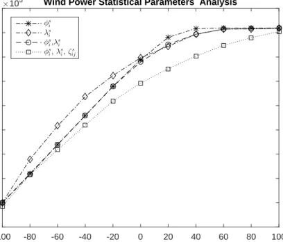
capacity varies from 0% - 100% . . . 29 3.1 Five areas power system configuration . . . 42 3.2 The effect of incorporating the wind power statistical data in DRO . 46 3.3 The effect ofφs

1 variation on WPG . . . 47

3.4 The effect ofλ1 variation on WPG . . . 48

3.5 The response ofζs

ij change on WPG . . . 49

3.6 The effect ofξs

24 variation on WPG . . . 50

3.7 The optimal allocation of WPG . . . 51 3.8 The optimal allocation of WPG with diffrent transmission lines

trans-fer capacity . . . 52 3.9 The effect of the generation failure rates on WPG . . . 53

4.1 Optimal wind and solar power allocation for different capacities in the

five-area system . . . 69

4.2 Overall EENS evaluation comparison . . . 70

5.1 Graphical example of capacity credit evaluation . . . 76

5.2 Capacity credit analysis of WPG in isolated system . . . 78

5.3 Capacity credit analysis of WPG in interconnected system . . . 79

5.4 Capacity credit analysis of SPG in isolated system . . . 81

5.5 Capacity credit analysis of SPG in interconnected system . . . 82

5.6 Capacity credit analysis of HWSPG in isolated system . . . 84

5.7 Capacity credit analysis of HWSPG in interconnected system . . . 85

5.8 Capacity credit analysis comparison . . . 87

5.9 Capacity credit analysis evaluation . . . 88

5.10 Penetration factor analysis Comparison . . . 89

LIST OF TABLES

TABLE Page

2.1 Power system data and the results . . . 27

3.1 Power system data and the DRO results . . . 43

3.2 DRO results of different wind statistical data . . . 45

4.1 The power system data . . . 67

4.2 The DRO results . . . 68

5.1 Capacity credit relation to the WPG penetration factor . . . 80

5.2 Capacity credit relation to the SPG penetration factor . . . 83

5.3 Capacity credit relation to the HWSPG penetration factor . . . 86

B.1 Wind data structure . . . 108

B.2 Generation capacity data structure . . . 109

B.3 Load data structure . . . 109

1. INTRODUCTION

1.1 Wind Power Generation

Wind power generation (WPG) is the most widely used and the fastest expand-ing renewable resource for electric power generation worldwide [1–3]. It shows a remarkable increase in growth rate over the past two decades [4], and it has become a primary source for electric power generation in several countries [5]. Furthermore, besides the issue of the global warming and the depletion of fossil fuels needed to generate electricity, the trend in the sector of the electric power industry is towards the investment in renewable energy resources [6], to accomplish goals such as carbon dioxide emission reduction, energy self-sufficiency, increasing the system reliability, prevent load curtailment and improving the social welfare [7].

Consequently, the dramatic expansion of WPG poses several challenges in terms of power system operation, since WPG is intermittent, uncertain and not fully dis-patchable, which requires extra attention to power system planning and operation studies with a particular emphasis on modeling the uncertainty of power system, to ideally perform economic dispatch, unit commitment and spinning reserve, as the generation should balance the load demand on a moment-by-moment basis keeping the operational constraints of both generation units and transmission lines networks with no violation [8–10]. So in long-term power system planning, an optimal de-cision to efficiently integrate a large-scale WPG into the power system besides the existing conventional generation has played a significant role in a reliable and eco-nomical operation for the entire power system [3, 11, 12], which indeed motivates to more development in planning procedures and techniques to examine a wide range of uncertainty representation methods [4,13].

1.2 Probabilistic Modeling of Uncertainty

Unlike conventional power generation, many renewable energy resources such as the wind or solar have a maximum power output that varies with time which is described by random variability [14]. Such uncertain behavior of the renewable energy resources increases the difficulties of power system operation, in which the generation should balance the load demand on a moment-by-moment basis keeping the operational constraints of both generation units and transmission lines networks with no violation [10]. To accommodate high penetration of variable energy resources in the power systems generation, the system is required to be more flexible to follow the variable net demand and deal with the uncertainties to maintain the reliability and the security of the system within the desired levels [15].

To cope with the uncertain nature imposed by the renewable energy resources and the electric power components, the application of probabilistic tool is useful to investigate and represent the uncertain system. [16]. The uncertain arbitrary variable can be modeled and described by the probability distribution functions (PDF), which is an important step to deal with the variability issue. The intensive meteorological observation of the wind and solar pattern to represent it in proper statistical parameters reduces the problem of uncertainty, and it assures the highest possible flexibility and availability needed to keep the load-generation balance during the operation [15]. In the next section, the methods and system models which are used to deal with system uncertainty are introduced.

1.3 Optimization Model under Uncertainty

It is important to develop a non-deterministic optimal wind power allocation framework which includes the uncertain nature of both the wind power availability and other random power system components. The method should be computa-tionally tractable and statistically consistent, for finding a flexible solution against different realizations of uncertainty representation. In power system operation and planning studies, several methodologies like scenario interpretation and probabilistic analysis have been developed to deal with the uncertainty of wind power.

Stochastic Programming (SP) [17], represents uncertain variables through scenar-ios based on the assumption that the exact probability distribution of wind power is available [11]. A high accuracy probability distribution function representation of the uncertain nature of variable generation has to be obtained in order to ideally apply SP, and that requires sufficient historical data which is not always available. The lack of sufficient data limits the ability of SP and deteriorates its performance [18].

Although this problem has been mitigated by introducing Robust Optimization (RO) [19,20], which can be used even with no availability of any distributions data pa-rameters, except some data which can preserve the system against a pre-determined uncertainty set [21], such approach drives the solution to be conservative [10]. RO models uncertainty as a deterministic set without any probabilistic information. It affords a robust solution that is preserved to any possible scenario of the uncertainty set, which is an essential perspective in the security-constrained electric power sys-tems planning, however, that would lead to a conservative and sometimes less effec-tive solution [22]. Furthermore, RO uses bounded intervals to handle a broad range of uncertainty sources in modeling the uncertain random variables.

un-certainty sources, since it only requires the relative variation intervals of uncertain variables rather than generating scenarios as applied in SP. Furthermore, RO is more conservative compared to SP. While the solution of RO is optimal for the worst case realization of uncertain variables, the solution of SP is optimal on average for a set of deterministic scenarios which capture the nature of uncertainty [12]. As an interme-diate methodology, Distributionally Robust Optimization (DRO) [23], is introduced to mitigate the limitations of SP and RO by providing a tractable approach to proba-bilistically include the available characteristic information of the uncertain variables in an ambiguity set [24–26], and it is less conservative by avoiding the extreme de-cision of totally neglecting the probability distribution of the random variables as applied in RO. The detailed procedure of the proposed approached is demonstrated in the following section.

1.4 Distributionally Robust Optimization

DRO has been recently applied in several power system problems to represent the uncertainty of random variables [10,27]. Its capability in probabilistic interpretation of the data-driven decision making is the bottom line behind its success [28]. DRO operates by including certain probabilistic information of the uncertain variables appropriately in the optimization modeling; it deals with the uncertain parameter as a random variable that tracks the stochastic nature by involving a family of probability distributions characteristics defined by an ambiguity set [29].

Compared to SP, which improve the optimal solution by minimizing the expecta-tion of the energy not served under the scenarios representaexpecta-tion of the system uncer-tainties following one distinct probability distribution, DRO overcomes the critical assumption in SP regarding the availability of the exact distribution information. Ad-ditionally, DRO resolves the computational difficulties addressed by the SP scenario

representation which requires decomposition and scenario selection algorithms [4,30]. On the other hand, the conventional RO achieves the objective under the worst-case energy not served over all possible realizations within a deterministic uncertainty set of the uncertain variables. It solves the issue of the scenarios interpretation proposed in SP, but it can not model indices in terms of the expected values and leads to more conservative solution by totally neglecting the probability distribution [20]. So, DRO is primarily the integrated robust practice of the stochastic programming. [22] which provides a moderate method to represent uncertainty in reliability based design optimization.

The objective of this research is to allocate a certain amount of renewable power genration in a multi-area power system to minimize the expected energy not served under the worst-case probability distribution that is characterized by the ambiguity set of the renewable power uncertainty and generator forced outages. The linear decision rule approximation [23, 31, 32] is used to restrict the second-stage recourse decisions to be affinely dependent on uncertain parameters as well as auxiliary ran-dom variables where the distributional statistical information of uncertain variables are represented, so that the overall problem can be solved in a tractable manner [33].

1.5 Monte Carlo Simulation for Generation Adequacy Evaluation

The sampling based Monte Carlo simulation (MCS) is utilized to perform the sensitivity analysis of the proposed renewable generation expansion design problem. This practice is widely used in the planning studies due to its simplicity in imple-menting and effectiveness in evaluating the proposed decisions. It is beneficial with calculating all required system operation information and reliability indices.

In general, this simulation approach offers more flexibility with handling the system’s operational conditions, because it allows for the scenarios representation

based simulation which should reflect all possible operational system states with sufficient number of scenarios to secure the convergence and provide accurate results for a fair evaluation of any stage of reliability analysis. Reliability indices like loss of load expectation (LOLE) and expected energy not served (EENS) are estimated using MCS. However, to yield a converged and trusted solution the MCS may need a long computational time to process such large number of scenarios.

In the sampling technique, the main procedure is to generate random samples of the system states including the wind power, conventional generation, and all other random variables of the system components according to their particular probability distributions. The other fixed information like the system configuration, operational limits, and the constraints are fixed for every iteration. Then after simulating a sufficient number of samples which lead to an acceptable value of the coefficient of variance (COV) for that distinct set of samples or scenarios, the reliability indices are then analytically calculated from those samples.

The convergence of the simulation occurs when the coefficient of variation of the calculated index from a set of samples lies within a consistent range, such range is set to be generally less or equal to 5%. Such convergence is strongly associated with the loss of load probability (LOLP) since the COV calculation depends on the events occurring on the power system. In a reliable power system, where the loss of load events happen relatively rarely, observing the variation requires a long computational time since the change is small due to the estimation of relatively low value of the LOLP, which makes the MCS more computationally challenging with a reliable power system.

A combination of optimization schemes incorporating with reliability evaluation is practiced in many types of planning and design problems. In [34], adequacy deter-mination of locational generation and transmission lines transfer capacities are

eval-uated. The optimization procedure is used for a planning investigation of any addi-tional expansion of both power generation and transmission lines. References [35,36] discusse an optimization procedure for generation expansion determination based on a reliability evaluation in multi-area power systems. The global decomposition approach is utilized to get a proper tradeoff between the cost and the power sys-tem reliability. The stochastic programming based optimization to represent the uncertainties in conventional generation, transmission lines and the load demands to evaluate the power generation expansion problem in the multi-area power system is introduced in [37–40]. A stochastic programming using Bender’s decomposition algorithm is used to optimize the transmission lines expansion problem with the high penetration of the wind power is investigated in [41]. All the above problems usu-ally seek for the solution that maximizes the system reliability and minimizing the planning or operational cost. Because of the system uncertainties presence during the reliability evaluation the system is classified to be a stochastic problem which requires more attention to probabilistic modeling of their components and find the optimization approach which takes this particular feature into account.

To construct the probability distribution function or the density function of the conventional generation availability using MCS, the historical information like failure rates and repair rates of all generation components have to be available.

1.6 Multi-Area Power System

When realizing a multi-area power system as a wide geographically connected regions with separated wind farms, the second and minute variations in a single area can be relieved by the smoothing effect of the other areas wind generation diversity which is accounted as an advantage in stabilizing the system operation while the wind power generation is appropriately distributed [15].

Multi-area power systems can be modeled as a network flow structure of multiple areas connected by tie lines where each area represents an electrical power system consisting of generators, transformers, transmission lines and load buses. Each area has its particular configuration with different component ratings and reliability based information like forced outages rate (FOR), mean up time and mean down time which allows finding the failure and repair rates to conduct the Monte Carlo simulation.

The generation system is modeled based on its discrete probability distribution function which can be constructed using Monte Carlo simulation or analytically using Markov chain by knowing its generation units capacities and their forced outage rates (FOR). In this research the Monte Carlo based simulation to construct the generation model is used for each area of the system. The load model is formed as load duration curve (LDC), such model is sufficient in the planning problem studies using non-sequential Monte Carlo based simulation, whereas the hourly model or chronological model is preferred in the operational type studies where the analysis at a small time scale is critical. However, in the planning problem which considers a large set of historical data to be analyzed, considering the chronological model will make the study of different realization for multiple case studies in a single year difficult and not practical due to the high computational time required to do the simulation.

Considerable attention therefore has been given to multi-area system reliability assessment while allocating wind power generation and which area should be rein-forced with wind power generation among other areas in the overall system [42]. The adoption of reliability evaluation and optimization schemes is utilized in many kinds of system planning and operation problems [43]. These problems usually search for the optimal solution that maximizes system reliability subjected to the operational constraints [8].

areas. Since each area generally follows a different probability distribution comparing to other far distance areas, such difference would fulfill the shortage of certain areas by the excess of others, which would enhance the generation adequacy and the overall power system reliability [9,44]. Moreover, the association of transmission constraints in the model would impose additional security obligations to ensure system reliability, since transmission constraints heavily influence the optimal precept for allocating the wind power generation in each area of the network [13]. The planning problem determines the percentage of investment committed to each area according to an overall specific budget that would minimize the expected energy not served in the entire system, which could mitigate the influence of outages, encourage affordable and stable market prices, and promote investments in sustain and more efficient manner [45].

1.7 Organization of the Dissertation

The dissertation is organized as follows. Chapter 2 describes the mathematical model of DRO based approach for wind farm allocation using the linear represen-tation of statistical wind power data; the proposed method is validated with a case study on a five-area power system. Chapter 3 improves the method introduced in Chapter 2 by applying further effective procedure in representing wind power data using second-order cone programming. Chapter 4 introduces the DRO based plan-ning scheme in allocating hybrid (the wind and solar) power generation system and how the diversity in utilizing the renewable power generation improves the power system reliability. Chapter 5 address the capacity credit evaluation using the an-alytical approach to estimate the effective load carrying of the installed renewable power generation units. The conclusion of the results in this dissertation is given in Chapter 6. The References and the appendixes are attached at the end.

2. WIND FARM ALLOCATION PLANNING PROBLEM

2.1 Linear Representation Formulation of Wind Power Statistical Parameters

2.1.1 A Two-Stage Wind Farm Allocation Model

The wind farm allocation model is formulated as a two-stage problem, where the wind power allocation decisions are made in the first stage, and the operation decisions are determined as the random wind power ˜www and the uncertain generator capacity ˜ppp are realized.

The first-stage wind power planning problem is expressed as follows.

min sup P∈F EP{L(xxx,w,ww˜ p˜pp)} (2.1) s.t. 0≤xi ≤Πi (2.2) X i∈I xi = Ω (2.3)

where xxx is the vector of first-stage decision variables, where xi represents the

wind power capacity placed in area i. The constraints (2.2) indicates that the wind capacity xi in each area is subject to an upper limitation Πi, due to geographic

conditions, environmental or social concerns. The total capacity of installed wind power for all areas in I is denoted by Ω in (2.3).

The objective function (2.1) minimizes the expected energy not served (EENS) under the worst-case distribution of ˜wwwand ˜ppp, which is denoted by_Pover anambiguity set _F. The detailed discussion on the ambiguity set _Fis given in the next subsection. The expression L(xxx, www, ppp) in (2.1) indicates the amount of energy not served for the wind farm allocation decisionxxxunder the wind power outcomewwwand the generation capacity realization ppp. It is expressed as the second-stage optimization problem

shown below. L(xxx,www, ppp) = min X s∈S X t∈T X i∈I T_tsls_it (2.4) s.t. xiwsi +q s it− X j∈J_if f_jits + X j∈Jt i f_ijts =Ds_it−l_its, ∀i∈ I,∀t ∈ T,∀s∈ S (2.5) −Fij ≤fijts ≤Fij, ∀j ∈ J_if,∀i∈ I,∀t∈ T,∀s∈ S (2.6) 0≤qs_it≤pi, ∀i∈ I,∀t ∈ T,∀s∈ S (2.7) ls_it≥0 ∀i∈ I,∀t∈ T,∀s ∈ S (2.8)

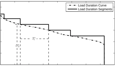
This formulation considers a set of wind power distributions, denoted by S, in order to capture the seasonal or day-night differences of wind power patterns [13]. The load duration curve under each wind power distribution type sis approximated by a segment expression, illustrated by an example in Fig. 2.1. The index of each load segment is denoted by t, and the setT is the set of all load segments [46–49].

For each time segmenttunder wind power distributions, the constantT_tsdenotes the duration of load segment t under wind power distribution type s, and Ds

it is the

corresponding load in areai. The variablesqs

itandlsitare the conventional generation

and load loss in area i, respectively, and the power transmitted from areaj to area i is denoted byfs

ijt. The objective function (2.4) indicates the amount of energy not

served over a year. The power balance in each area is enforced by equation (2.5). Constraint (2.6) suggests that the power flow from area ito area j should be within the capacity of transmission lines. The conventional generation q_its should also be constrained below the available capacitypi, as expressed by (2.7). The last inequality

0 300 600 900 1200 1500 1800 2100 2400 0 20 40 60 80 100

Hours per Year

Demand as a Percentage of the Peak Load

Ts t

Ds it

Load Duration Curve Load Duration Segments

Figure 2.1: Illustration of the segment approximation of load duration, as an example of the RTS-1996 load data in Spring

(2.8) indicates that the loss of load ls

it should be nonnegative.

2.1.2 Ambiguity Set

The proposed wind power planning formulation in this research addresses two types of uncertainties: the random wind power generation and the forced outages of generators. Unlike the stochastic programming approaches that optimize the expec-tation based on one underlying distribution, this distributionally robust optimization model manages system uncertainties by considering a family of distributions, defined by an ambiguity set [8, 50]. against the incomplete or the lack of accuracy of distri-bution information.

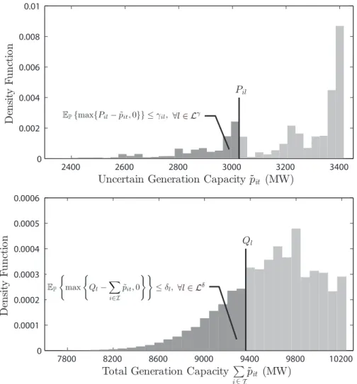
a family of wind power distributions. Pr{www˜ ∈ W}= 1 (2.9) EP{w˜si}= ¯w s i,∀i∈ I,∀s∈ S (2.10) EP{max{w˜si −W s il,0}} ≤α s il, ∀i∈ I,∀l ∈ Lα_{,∀s∈ S (2.11)} EP n max{w˜s_i + ˜w_js−w¯_is−w¯_js,0}o≤β_ijs, ∀j < i∈ I,∀s∈ S (2.12)

The equation (2.9) suggests that the vector of random wind power generation is constrained within an uncertainty set W, which is designed similarly to that in the conventional robust optimization problems. In this research, the uncertainty set W is defined as (2.13). W = ( w ww∈_R|I|×|S| : 0_≤ws i ≤1, ∀i∈ I,∀s∈ S ) (2.13)

The equation (2.10) implies that the expected value of each ˜ws

i is ¯wis, and the

next inequality (2.11) incorporates distribution informationαs_ilin terms the absolute deviation of ˜w_is around a selected wind power level W_ils into the ambiguity set. Be-cause the distribution of wind power is typically skewed and long-tailed [51, 52], or even bimodal [53,54], the expression (2.11) is used for multiple wind power levelsWs il

in order to capture the variability and skewness of wind power distributions, illus-trated by the upper plot in Fig. 2.2. As more wind power levels are considered, the distributions of wind power generation can be represented in a more precise manner and the worst-case distribution should be less adverse, leading to less conservative solutions [55, 56]. The last expression (2.12) is used to limit the mean absolute

de-viation of the generation summation from two wind farms below a constant βs ij, as

illustrated by the lower plot in Fig. 2.2. This inequality implicitly incorporates the information on the correlation between wind farms into the ambiguity set. If the power output from two wind farms are negatively correlated, the constant βs

ij is

likely to be smaller, and positive correlation commonly lead to largerβs

ij. Notice that

unlike the stochastic programming approaches that consider one wind power distri-bution by the scenario-representation, the proposed uncertainty model addresses a family of distributions characterized by the parameters ¯ws_i,αs_il and β_ijs, which can be calculated straightforwardly based on the historical data, thus more practical than identifying the exact distribution of wind power generation.

The uncertain conventional generation capacities ˜ppp can be modeled in a similar way, as expressed by (2.14)-(2.17). Pr{˜ppp∈ P}= 1 (2.14) EP{p˜i}= ¯pi, ∀i∈ I (2.15) EP{max{Pil−p˜i,0}} ≤γil, ∀i∈ I,∀l ∈ Lγ (2.16) EP ( max ( Ql− X i∈I ˜ pi,0 )) ≤δl, ∀l ∈ Lδ (2.17)

The first expression (2.14) implies that the vector of uncertain generation capacity is constrained within an uncertainty set P, which is defined as follows:

P = ( p pp∈_R|I| : _pmin i ≤pi ≤pmaxi , ∀i∈ I ) (2.18)

Similar to (2.10), the second equation (2.15) defines the expected value of the uncertain generation capacity ˜pi. The third expression (2.16) selects a set of

0 20 40 60 80 100

Random Wind Powerw˜s

it (as a percentage of capacity)

D en si ty F u n ct io n Ws il W s i(l+1) 0 20 40 60 80 100

Random Wind Powerw˜_its +w˜_jts (as a percentage of capacity summation)

D en si ty F u n ct io n Mean Value: wis+wsj

Histogram of Wind Power

Wind Power fitted by Beta Distribution Histogram of Wind Power

Wind Power fitted by Beta Distribution

Figure 2.2: Illustration of the expressions that characterize the wind power distribu-tions, based on an example of California wind farms in Spring

part of Pil −p˜i below a constant γil, as illustrated by the upper plot in Fig. 2.3.

The last expression characterizes the distribution of the total generation capacity in the same fashion, i.e., the expected value of the positive part of Ql − P

i∈I

pi is

constrained below a constant δl, where Ql is the selected generation level, and Lδ

is the set of all selected levels, as shown in the lower plot of Fig. 2.3. Note that both the expressions (2.16) and (2.17) are utilized to incorporate the information on distribution patterns of generation capacities into the ambiguity set, and this

uncer-tainty model is more practical than conventional stochastic programming methods because there is no need to attain the detailed data on the exact generation capacity distribution, which is usually inaccessible or too complex to represent. Instead, we only need to calculate the constants γil and δl based on the historical data and the

selected generation levels. Including more generation levels into the sets Lγ and _Lδ

will improve the precision of characterizing the distribution of generation capacities in the ambiguity set.

By combining the wind power uncertainty model (2.9)-(2.12) and the generation capacity expressions (2.14)-(2.17), the overall ambiguity set, denoted by F, can be

formulated as (2.19).

Based on the ambiguity set presented above, the proposed wind power allocation model minimizes the expected energy not serve under the worst-case distribution. In the next section, this two-stage formulation is reformulated into a tractable linear programming problem using the linear decision rule approximation.

F=                                                      P∈ Q0 R|I|×|S|×R|I| : ˜ www∈_R|I|×|S| Pr{www˜ ∈ W}= 1 EP{w˜si}= ¯wsi EP{max{w˜si −Wils,0}} ≤αsil,∀i∈ I EP n max{w˜s_i + ˜ws_j −w¯_is−w¯_js,0}o≤β_ijs ˜ ppp∈_R|I| Pr{pp˜p∈ P}= 1 EP{p˜i}= ¯pi EP{max{Pil−p˜i,0}} ≤γil EP ( max ( Ql− P i∈I ˜ pi,0 )) ≤δl                                                      (2.19)

2400 2600 2800 3000 3200 3400 0 0.002 0.004 0.006 0.008 0.01 Pil

Uncertain Generation Capacityp˜it (MW)

D en si ty F u n ct io n 7800 8200 8600 9000 9400 9800 10200 0 0.0001 0.0002 0.0003 0.0004 0.0005 0.0006 Ql

Total Generation CapacityP i∈I ˜ pit (MW) D en si ty F u n ct io n

Figure 2.3: Illustration of the expressions that characterize the generation capacity distributions, based on an example of the Reliability Test System 1996

2.2 Problem Solving Procedure

2.2.1 Compact Matrix Formulation

The formulation presented in the previous section is expressed in more general compact matrix forms, in order to facilitate the discussion of the reformulation proce-dure. In this section, vectors are represented by bold lower case letters, and matrices are represented by bold capital letters. Elements of vectors or matrices are denoted

by regular letters with subscripts indicating the indices. The first-stage decisions are still denoted by xxx, and the set of all first-stage decisions is named as N1. All

second-stage decisions, including qs

it, fijts , and lits, are represented by a vectoryyy, and

the set of all second-stage decision variables is denoted byN2. The random variables

wwwandpppare combined as a vectorzzz ∈_R|V|_{, whereV is the set of all random variables.}

The first-stage problem (2.1)-(2.3) is then expressed as the matrix form (2.20)-(2.21). min sup P∈F EP{L(xxx,zzz˜)} (2.20) s.t.AxAxAx≤bbb (2.21) with xxx∈ _R|N1|, _AAA∈ R|M1|×|N1| and _bbb ∈ R|M1|, where M

1 is the set of all first-stage

constraints.

The second-stage problem (2.4)-(2.8) used for calculating functionL(xxx, zzz) is given as (2.22)-(2.23). L(xxx, zzz) = min qqqTyyy (2.22) s.t.CCC(zzz) +DyDyDy≤ddd(zzz) (2.23) with qqq ∈ _R|N2|, _CCC(_zzz) ∈ R|M2|×|N1|, _DDD ∈ R|M2|×|N2|, and _ddd(_zzz) ∈ R|M2|, where M 2

represents the set of all second-stage constraints. Notice that both the left-hand-side constraints matrix CCC(zzz) and the right-hand-side coefficient vector ddd(zzz) are affected by the random variables zzz. They are commonly assumed to be the following linear

affine form [33]. C C C(zzz) =CCC0+X v∈V CCCvzv (2.24) d d d(zzz) =ddd0+X v∈V d d dvzv (2.25) with constants CCC0_{, CCC}v _∈

R|M2|×|N1|, and ddd0, dddv ∈ R|M2|. The other parameters in

matrix DDD are independent from the random variables, hence is the case of fixed recourse [17].

The ambiguity set (2.19) is expressed as the compact matrix form below.

F=                              P∈ Q0 R|V| : ˜ zzz ∈_R|V| Pr{zzz˜∈ Z}= 1 EP{z˜v}= ¯zv, ∀v ∈ V EP{gk(˜zzz)} ≤σk,∀k ∈ K                              (2.26)

The second line of (2.26) suggests that the vector of random variables is constrained within an uncertainty set Z, which is the combination of set W in (2.9) and P in (2.14). The third line of (2.26) is the generalized form of expressions (2.10) and (2.15), used to define the expected value of random variables. The last line in (2.26) is the compact matrix form of the remaining inequalities in (2.19). The function gk(˜zzz) in (2.26) generalizes the absolute deviation and the positive part expression in

(2.11)-(2.12) and (2.16)-(2.17), and all constants αs

il, βijs, γil, and δl are represented

2.2.2 Extended Ambiguity Set

In this subsection, the ambiguity set F in (2.26) is extended in (2.27) by by

introducing auxiliary variables ˜uk that express the upper bound of each function

gk(˜zzz) into the formulation.

¯ F=                              Q∈ Q0 R|V|×R|K| : (˜zzz,uuu˜)∈_R|V|_× R|K| Prn (˜zzz,uuu˜)∈Z¯o= 1 EP{z˜v}= ¯zv,∀v ∈ V EP{u˜k} ≤σk,∀k∈ K                              (2.27)

where ¯Z is the extended form of the uncertainty set Z, expressed as (2.28).

¯ Z =                    (zzz, uuu)∈_R|V|_× R|K|: zzz ∈ Z gk(zzz)≤uk, ∀k ∈ K uk ≤max z zz∈Z gk(zzz),∀k ∈ K                    (2.28)

Note that the uncertainty setZ are defined by linear constraints (2.9) and (2.14), and the function gk(zzz) is also linear representable because it is expressed as the

absolute deviation in (2.11)-(2.12) and the positive part in (2.16)-(2.17). As a result, the extended support set ¯Z in (2.28) can be written as the following linear matrix form. ¯ Z = ( (zzz, uuu)∈_R|V|×_R|K| : _{F zF zF z+HuHuHu≤hhh} ) (2.29) with FFF ∈ _R|R|×|V|_{,HHH ∈}

R|R|×|K|, and hhh∈R|R|, whereR denotes the set of all linear

The extended ambiguity set ¯F and the uncertainty set ¯Z are utilized in the

next subsection to transform the two-stage wind power planning problem into a computationally tractable formulation.

2.2.3 Reformulation with the Generalized Linear Decision Rule

The exact solution for this two-stage optimization problem is generally intractable, because the expectation of L(xxx,zzz˜) must be calculated by solving the second-stage recourse problem (2.22)-(2.23) under all realizations of random variables ˜zzz. This difficulty is normally addressed by linear decision rule techniques [32, 33, 57]. In this approach, we utilize the generalized linear decision rule [32] to approximate the recourse decision yyy by a linear affine function of some system uncertainties zzz and auxiliary variablesuuu, expressed as equation (2.30).

yn(zzz, uuu) = yn0 + X v∈Vn yz_nvzv+ X k∈Kn y_nku uk (2.30)

with (zzz, uuu)∈Z¯, recalling that ¯Z is the extended support set defined in (2.28). that affect the recourse decision yn, and similarly, the set Kn is a subset of K, involving

all auxiliary variables that influence decision yn. It is pointed out by [32] that the

problem size can be reduced if fewer random and auxiliary variables are included in each decision rule, the recourse decision rule thus assumes that decision yn is a

function of the random and auxiliary variables for the same load segment and wind power distribution type as yn. The sets of all random variables zzz and auxiliary

variables uuu that are incorporated into the decision rule function yn are respectively

denoted by Vn and Kn in (2.30). This assumption should be valid because the

occurrence of load loss under every load segment and wind power distribution type is independent, e.g., the energy not served at wind nights are unlikely to be affected

by wind power outcomes during the day time in summer. yn is denoted byKn.

It has also been shown in reference [32] that the ambiguity set F is equivalent

to the set of marginal distributions of uncertain variables ˜zzz under _Q, for all _Q ∈_F¯, where ¯F is the extended ambiguity set (2.27) discussed in the previous subsection.

We can hence derive the following equation.

max P∈F EP n qqqTyyy(˜zzz,uuu˜)o= max Q∈F¯ EQ n qqqTyyy(˜zzz,uuu˜)o (2.31)

for some decision rules yyy(zzz, uuu) that are feasible under all realizations of system un-certainties ˜zzz. The original two-stage problem can be therefore transformed into the following formulation by replacing the recourse decisionyyyby the linear decision rule approximationyyy(zzz, uuu). min max Q∈¯F qqqTyyy(˜zzz,uuu˜) (2.32) s.tAxAxAx≤bbb (2.33) CCC(zzz)xxx+DyDyDy(zzz, uuu)≤ddd(zzz), ∀(zzz, uuu)∈Z¯ (2.34)

The optimization problem (2.32)-(2.34) is then reformulated into the following robust optimization problem by taking the dual of the inner maximization of the objective

(2.32). min ρ+ ¯zzzTηηη+σσσTλλλ (2.35) s.t.AxAxAx ≤bbb (2.36) ρ+zzzTηηη+uuuTλλλ≥qqqTyyy(zzz, uuu), ∀(zzz, uuu)∈Z¯ (2.37) C C C(zzz)xxx+DyDyDy(zzz, uuu)≤ddd(zzz), ∀(zzz, uuu)∈Z¯ (2.38) λ λ λ ≤0, ρ∈_R, ηηη∈_R|S|, λλλ ∈_R|K| (2.39)

where ρ is the dual variable associated with the underlying implication that the probability summation is one, and the other dual variablesηηη and λλλ are respectively associated with the third and fourth line of the ambiguity set ¯F in (2.27).

It can be seen that the problem (2.35)-(2.39) is a typical robust counterpart, which leads to an equivalent linear programming formulation. Let Nz

v denote the

set of recourse decisions that are affected by random variable ˜zv, and Nku be the set

of recourse decisions affected by the auxiliary variable ˜uk. Both sets can be derived

program can be thus expressed as (2.40)-(2.49). min ρ+ ¯zzzTηηη+σσσTλλλ (2.40) s.t.AxAxAx≤bbb (2.41) ρ−qqqTyyy0 ≥hhhTπππ0 (2.42) X r∈R Frvπr0 = X n∈Nz v qnyznv−ηv,∀v ∈ V, ∀m∈ M2 (2.43) X r∈R Hrkπ0r = X n∈Nu k qnynku −λk,∀k ∈ K,∀m ∈ M2 (2.44) X r∈R hrπrm ≤d 0 m− X n∈N1 C_mn0 xn− X n∈N2 Dmnyn, ∀m∈ M2 (2.45) X r∈R Frvπrm = X n∈N1 C_mnv xn−dvm+ X n∈Nz v Dmnynkz , ∀v ∈ V,∀m∈ M2 (2.46) X r∈R Hrkπmr = X n∈Nu k Dmnyknu , ∀k ∈ K,∀m∈ M2 (2.47) λλλ≤0, πππ0 ≤0, πππm ≤0, ∀m∈ M2 (2.48) ρ∈_R, ηηη∈_R|S|, λλλ∈_R|K|, πππ0, πππm ∈_R|R|, ∀m ∈ M2 (2.49)

model. Case studies are presented in the next section to demonstrate the effectiveness and tractability of the proposed method.

The uncertain constraints (2.38) and (2.39) are reformulated into (2.42)-(2.44) and (2.45)-(2.47), respectively, by considering the dual variable πππ0 and _πππm associated

with constraints in the extended support Z¯ in (2.28).

It can be seen that the two-stage wind power planning model is reformulated into a tractable linear programming problem (2.40)-(2.49). By applying the linear decision rule approximation, the resultant linear optimization formulation might be more conservative, but it is much easier to be solved than the original two-stage

2.3 Five-Area System Case Study

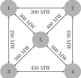
To validate the proposed DRO technique on the wind farm allocation planning problem, a five-area power system (Fig. 2.4) is used to allocate a certain amount of megawatts, which is formerly determined by the power generation entity according to their budget. In this case study, 1500 MW of WPG as an example is optimally

1 2 3 4 5 200 MW 250 MW 300 MW 350 MW 400MW 450 MW 500MW 600 MW

Figure 2.4: Five areas power system configuration and transmission lines transfer capacities

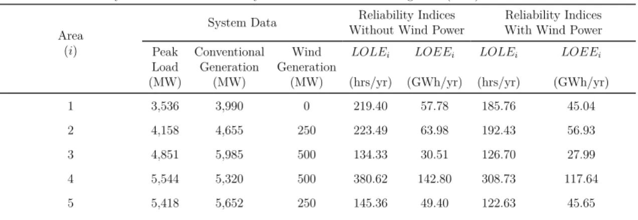
distributed within the system using the DRO framework to utilize the maximum obtainable wind power resources so that the minimum EENS is attained. The power system configuration of each area follows the IEEE RTS system [58] with different generation and load levels that distinguish the areas from each other. The power system data and the case study results are shown in the first part of TABLE 2.1. After assigning the optimal WPG in the system, random sampling Monte Carlo simulation [46] is performed to validate the results and to calculate the reliability indices for each area such as loss of load expectation (LOEEi), loss of energy expectation (LOEEi)

and the entire system reliability index EENS to evaluate the system after WPG integration.

Table 2.1: Power system data and the results

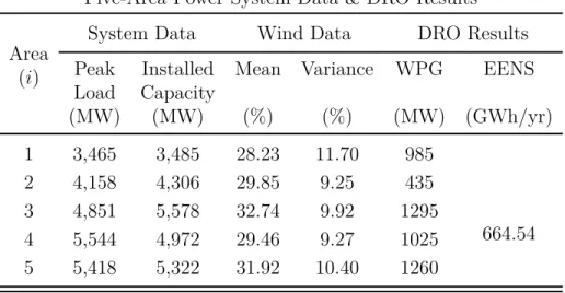
Power System Data and Reliability Assessment for Distributing 1500 (MW) of Wind Power Area

(i)

System Data _{Without Wind Power}Reliability Indices Reliability Indices_{With Wind Power} Peak Load (MW) Conventional Generation (MW) Wind Generation (MW) LOLEi (hrs/yr) LOEEi (GWh/yr) LOLEi (hrs/yr) LOEEi (GWh/yr) 1 3,536 3,990 0 219.40 57.78 185.76 45.04 2 4,158 4,655 250 223.49 63.98 192.43 56.93 3 4,851 5,985 500 134.33 30.51 126.70 27.99 4 5,544 5,320 500 380.62 142.80 308.73 117.64 5 5,418 5,652 250 145.36 49.40 122.63 45.65

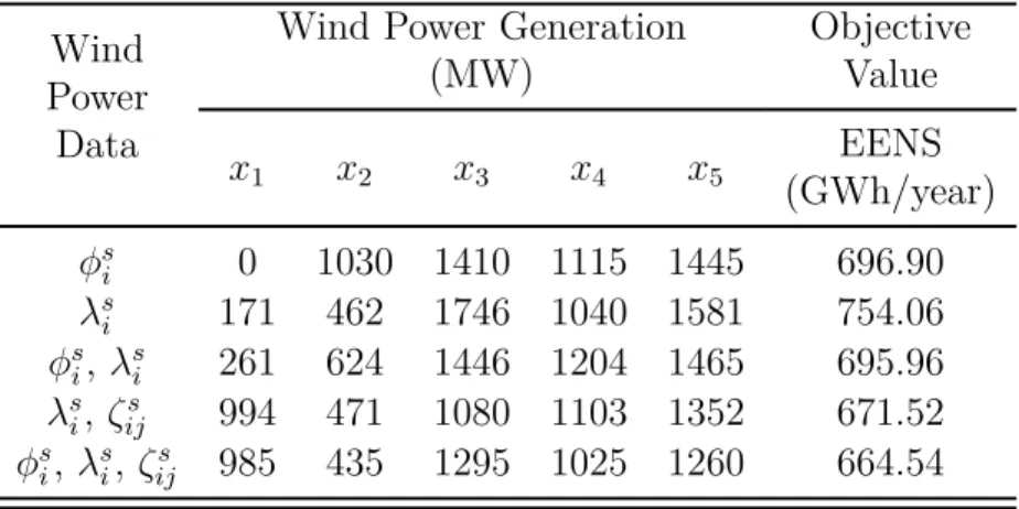
The Results of Optimal Wind Power Allocation for Different Probability Distribution Data Used in DRO Wind Power Probability

Distribution Data

Wind Generation (MW) Reliability Indices

x1 x2 x3 x4 x5 _(GWh/year)EENS

αs

il 0 119 500 500 381 803.57

αs

il,βijs 0 250 500 500 250 139.36

The second part of TABLE 2.1 demonstrates how the robustness of the decisions improves when more probability distribution information about the system variables is provided. This enhances the results and gives better intuition about the main data needed to accomplish such planning studies. According to this specific example, the proposed approach based on the information provided excludes area 1 from any investment in WPG (x1 = 0) for the given limited budget. Several factors control

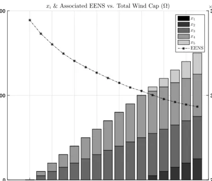
-200 0 200 400 600 800 1000 1200 1400 1600 Optimal Allocation of Wind Power for Diffrent (Ω) in MW

0 1000 2000 W in d P ow er C ap ac it y ( Ω ) in M W

xi& Associated EENS vs. Total Wind Cap (Ω)

2.5 3 3.5 E x p ec te d E n er gy N ot S er ve rd (E E N S ) in M W h /y ea r ×105 x₁ x₂ x₃ x4 x5 EENS

Figure 2.5: The optimal allocation of WPG when the total wind capacity (Ω) varies from 0-1500 MW

area 1, which is reflected in better reliability indices compared to other areas with no wind power. Furthermore, it has the lowest wind power availability among other areas represented in the wind resources statistical parameters such as ¯ws₁, αs_1l and βs

1j. Moreover, area 1 has 750 MW of transmission transfer capacity from other

neighboring areas, which allows their excess power to be delivered to it in case of generation shortages. Referring to Fig. 2.5, which illustrates that area 1 is not assigned with any WPG in all the cases of Ω from 0 MW to 1500 MW, except in a limited manner when there is no interconnection with other areas Fig. 2.6.

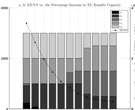
The transmission lines transfer capacities between areas apparently affect the op-timal planning decisions. Fig. 2.6 explains the relationship between the transmission transfer capacity and the allocation of the WPG in each area. It shows that with

0 10 20 30 40 50 60 70 80 90 100

Optimal Allocation of Wind Power for Diffrent Transmission Lines Transfer Capacity

0 1000 2000 W in d P ow er C ap ac it y ( Ω ) in M W

x_i&EEN S_{vs. the Percentage Increase in TL Transfer Capacity}

0 2 4 E x p ec te d E n er gy N ot S er ve rd (E E N S ) in M W h /y ea r ×106 x₁ x₂ x₃ x4 x₅ EENS

Figure 2.6: The optimal allocation of WPG when the transmission lines transfer capacity varies from 0% - 100%

a fixed amount of WPG, the EENS decreases as the transfer capacity increases and the WPG is uniquely distributed with different power transfer capability. Eventually, the results reveal an extraordinary reliability improvement with the interconnected power system, and the utilization of the renewable resources is improved, especially with a negatively correlated wind power availability between areas. Eventually, the results show an extraordinary reliability improvement in area 1 after installing just 5.85% of the total system’s generation capacity as a WPG to its interconnected areas by 15.13%, 15.33% and 22.05% decrees inLOLP1,LOLE1 andLOEE1 respectively.

in a nutshell, the multi-area power system gets benefit from the investment in WPG by decreasing in EENS by around 14.94%, and with the interconnecting system the utilization of the renewable resources is increased. The wind power statistical

param-etersαs

il andβijs which are used in the problem formulation are linear in order to gain

the advantages of the linear programming optimization which is convex and can be easily solved using simplex method. However, this technique represents wind data in an approximate linear formatting which requires a lot of piece-wise data segments to construct the wind power probability distribution function. As a result, additional standard wind power parameters such as wind power mean absolute deviation, vari-ance and covarivari-ance are introduced, since the varivari-ance and covarivari-ance are nonlinear parameters which convert the problem to a second order cone programming which is quadratically constrained linear program, it is convex and it can be solved using interior point method. This approach will be discussed in the next chapter.

3. NONLINEAR FORMULATION OF WIND FARM ALLOCATION PLANNING PROBLEM

3.1 Nonlinear Representation of Wind Power Statistical Parameters

3.1.1 A Two-Stage Wind Farm Allocation Model

Similar to the previous chapter, two types of uncertainties are addressed in the proposed wind power planning formulation: the random wind power generation ˜www and the available thermal generation capacity ˜ppp. The model is formulated as a two-stage problem where the wind power allocation decisions are made in the first two-stage and the operation decisions are determined as the ˜wwwand ˜pppare realized.The first-stage wind power planning problem is expressed as follows:

min sup P∈F EP{L(xxx,w,ww˜ p˜pp)} (3.1) s.t. 0≤xi ≤Πi (3.2) X i∈I xi = Ω (3.3)

wherexxxis the vector of first-stage decision variables and each xi represents the wind

power capacity in area i. The constraints (3.2) indicate that the wind capacity xi

in each area is subject to an upper limitation Πi due to geographic conditions and

environmental or social concerns. The total capacity of installed wind power for all areas in I is denoted by Ω in (3.3). The objective function (3.1) minimizes the expected energy not served (EENS) under the worst-case distribution of ˜www and ˜ppp, which is denoted by P, over an ambiguity set F. The expression L(xxx, www, ppp) in (3.1)

under the wind power outcome www and the available generation capacity realization ppp. It is expressed as the second-stage optimization problem shown in Section 2.1.1.

3.1.2 Ambiguity Set

The DRO model address system uncertainties by considering a family of distribu-tions, defined by an ambiguity set F [8, 50]. In this section, the power distributions

are represented using some standard statistical data representation. The expres-sions (3.4)-(3.8) are applied in the ambiguity set to define a family of wind power distributions. P{www˜ ∈ W}= 1 (3.4) EP{w˜si}= ¯wsi,∀i∈ I,∀s∈ S (3.5) EP{|w˜si −w¯ s i|} ≤φ s i,∀i∈ I,∀s∈ S (3.6) EP n ( ˜w_is−w¯s_i)2o≤λs_i,∀i∈ I,∀s ∈ S (3.7) EP n ( ˜w_is+ ˜ws_j −w¯_is−w¯_js)2o≤λs_i +λs_j + 2ζ_ijs, ∀j < i∈ I,∀s∈ S (3.8)

Equation (3.4) suggests that the vector of random wind power generation is con-strained within a support set W, which is designed similarly to that in the con-ventional RO problems. In this research, the support set W is defined by equation (3.9): W = ( w ww∈_R|I|×|S| : 0_≤ws i ≤1, ∀i∈ I,∀s∈ S ) (3.9)

Equation (3.5) implies that the expected value of each ˜ws

i is ¯wis, and the next

inequality (3.6) suggests that the mean absolute deviation of ˜ws

to φis_{. Similarly, constraints (3.7) suggest that the variance of ˜w}s

i is no higher

than the constant λs

i. The last expression (3.8) implies that the covariance between

˜ ws

i and ˜wsj is limited below ζijs. It can be seen that constraints (3.4)-(3.8) in the

ambiguity set attempts to capture the location, spread, and dependence of random wind power generation in terms of basic statistical measures, such as expectations, mean absolute deviations, variances and covariances. Such parameters should be much easier to estimate than the exact probability distribution.

The available conventional generation capacity ˜ppp is modeled exactly as applied in the previous chapter, by the equations (3.10)-(3.13):

P{p˜pp∈ P}= 1 (3.10) EP{p˜i}= ¯pi, ∀i∈ I (3.11) EP{max{Pil−p˜i,0}} ≤γil, ∀i∈ I,∀l ∈ Lγ (3.12) EP ( max ( Ql− X i∈I ˜ pi,0 )) ≤δl, ∀l ∈ Lδ (3.13)

The first expression (3.10) implies that the vector of uncertain generation capacity is constrained within a support set P, which is defined as follows:

P = ( p pp∈_R|I| : _pmin i ≤pi ≤pmaxi , ∀i∈ I ) (3.14)

By combining the wind power uncertainty model (3.4)-(3.8) and the generation capacity expressions (3.10)-(3.13), the overall F can be formulated as (3.15). In the

next section, this two-stage formulation is reformulated into a tractable second-order cone programming problem using linear decision rule approximations.

F=                                                            P∈ Q0 R|I|×|S|×R|I| : ˜ www∈_R|I|×|S| P{www˜ ∈ W}= 1 EP{w˜si}= ¯wsi EP{|w˜si −w¯is|} ≤φsi EP{( ˜wsi −w¯is)2} ≤λsi EP n ( ˜ws i + ˜wsj −w¯is−w¯sj)2 o ≤λs i +λsj+ 2ζijs ˜ ppp∈_R|I| P{p˜pp∈ P}= 1 EP{p˜i}= ¯pi EP{max{Pil−p˜i,0}} ≤γil EP ( max ( Ql− P i∈I ˜ pi,0 )) ≤δl                                                            (3.15) 3.2 Problem Reformulation

3.2.1 Compact Matrix Formulation

The formulation presented in the previous section is expressed in more general compact matrix forms in order to facilitate the discussion of the reformulation proce-dure. In this section, vectors and matrices are represented by bold lowercase letters. Entries of vectors or matrices are denoted by regular letters with subscripts indicat-ing the indices. The first-stage decisions are still denoted by xxx ∈ _R|N1|, where _N

1

is the set of all first-stage decisions. All second-stage decisions, including qs it, fijts ,

and ls

it, are represented by a vectoryyy∈R

|N2|, whereN

2 is the set of all second-stage

decisions. Random variables www and pppare combined as