VISA: Virtual Scanning Algorithm for Dynamic
Protection of Road Networks
Jaehoon Jeong, Yu Gu, Tian He and David Du
Department of Computer Science & Engineering, University of Minnesota Email:{jjeong,yugu,tianhe,du}@cs.umn.edu
Abstract—This paper proposes a VIrtual Scanning Algorithm
(VISA), tailored and optimized for road network surveillance. Our design uniquely leverages upon the facts that (i) the movement of targets (e.g., vehicles) is confined within roadways and (ii) the road network maps are normally known. We guarantee the detection of moving targets before they reach designated protection points (such as temporary base camps), while maximizing the lifetime of the sensor network. The main idea of this work is virtual scan – waves of sensing activities scheduled for road network protection. We provide design-space analysis on the performance of virtual scan in terms of lifetime and average detection delay. Importantly, to our knowledge, this is the first work to study how toguaranteetarget detection while sensor network deteriorates, using a novel hole handling technique. Through theoretical analysis and extensive simulation, it is shown that a surveillance system, using our design, sustains orders-of-magnitude longer lifetime than full coverage algorithms, and as much as ten times longer than legacy duty cycling algorithms.
I. INTRODUCTION
Surveillance for critical infrastructure and areas is regarded as one of the most practical applications of wireless sensor networks (WSNs). So far, most of WSN surveillance systems have focused on surveillance for two-dimensional spaces, such as open battlefields [1]–[4]. Research on road network surveillance, however, is very limited. In modern warfare, roadways (as fast maneuver paths) are vantage areas for military surveillance and operations. Clearly, surveillance in a road network is significantly different, because (i) the movement of targets (e.g., vehicles) is confined within road segments, and (ii) the road network maps are normally known (e.g., from Google Earth and Yahoo Maps). We argue that legacy solutions, which are not tailored for road networks, lead to suboptimal performance.
This paper proposes a novel sensing scheduling algorithm for target intrusion detection, utilizing the unique features of road networks. Specifically, we focus on supporting military operations with fast, infrastructure-free deployment. As shown in Figure 1(a), we guarantee the detection of targets, entering from entrance points, before they reach one of protection points; in modern warfare, battlefield situational awareness requires both entrance points and protections points (e.g., temporary base camps) to be assigned and changed on demand for fast military maneuver within a road network. Therefore, we cannot place sensor gatesa priori
before protection points for intrusion detection. Instead, a road-network-wide deployment is needed.
A straightforward solution for road network surveillance isduty cycling, in which nodes wake up simultaneously for w seconds (the minimum working time before reliable detection can be reported) and then the whole network remains silent forT seconds. The detection is guaranteed if it takes more thanT seconds for a target to travel along the shortest path between any pair of entrance
Entrance Point Protection Point
4 2 1 2 3 1 2 3 4 4
(a) Protected Road Network
E E E E P P P P split merge Sensors wake up consecutively
Scan
Detect!
Road Intersection Sensing Scan
1 2 3 1 2 3 4 4
(b) Concept of Virtual Scanning Fig. 1. Road Network Surveillance
points and protection points; this duty-cycling-based algorithm performs much better in terms of system lifetime than traditional full coverage algorithms [1]–[4] in road networks. This is because the duty cycling algorithm allows the whole network to be silent completely for T seconds everywseconds, but the full coverage algorithms (e.g., the one covers all intersections) require at least one subset of sensors to be active at any given point time, taking no advantage of the linear structure of road networks.
In this paper, we present a novel scan-based algorithm, which improves further energy efficiency of surveillance in road net-works. As shown in Figure 1(b), sensors wake up one by one for w seconds along road segments, creating waves of sensing activities, called virtual scanning. Waves propagate from one (or multiple) protection point P, split at the intersections, and merge along the route until they scan all of the road segments under surveillance. Our study reveals that this scan-based method can achieve significantly better performance (e.g., ten times system lifetime) than duty cycling algorithms. The concept of virtual scan-ning is simple, however, in-depth design is very challenging due to a set of practical issues we consider in this paper. Particularly, we investigate (i) how to optimize the network-wide silent durationT
between scan waves, (ii) how to coordinate the working schedules of individual sensors during the scan, and (iii) how to deal with sensing holes due to unbalanced initial node deployment, node failure and the depletion of node energy over time. Specifically, the intellectual contributions in this paper are as follows:
• A new architecture for surveillance in road networks. VISA
is the first work tailored for road networks, leading to orders-of-magnitude longer system life for target intrusion detection, using a novel scan-based algorithm.
• A sensing scheduling algorithm for an arbitrary road network. The working schedule of each sensor (i.e., when to wake up) is constructed in a decentralized way. The network-wide silent duration is computed by VISAscheduler and naturally disseminated along with sensing waves to the nodes.
• An optimal sensing hole handling algorithm for uncovered road segments. The VISA scheduler deals with both the initial sensing holes at the deployment time as well as the sensing holes due to the heterogeneous energy budget among sensors by optimally labeling additionalpseudoprotection or entrance points.
The rest of this paper is organized as follows: Section II describes the problem formulation. Section III explains the VISA
system design. Section IV evaluates our algorithm through simula-tion. We summarize related work in Section V and then conclude this paper with future work in Section VI.
II. PROBLEMFORMULATION
The problem is to maximize the lifetime of a sensor network, while ensuring all intruding targets are detected before they reach protection points. For clarity, this section explains the basic idea of virtual scanning, using one road segment, and then we extend our design to arbitrary road networks in Section III.
Dense area Sparse area Dense area Road Segment Length = l E 1 2 3 n n-1n-2 . . . . . . P . . .
Fig. 2. Randomized Linear Deployment
A. Virtual Scanning for Surveillance
We assumensensors are randomly placed on a road segment of length l. Each sensor has a conservative sensing circle of radius
r, which is long enough to cover the width of the road. This assumption holds true for most commercially available sensors (e.g., PIR sensors can detect moving car 60∼100 feet away). Therefore, we can represent sensing coverage using a linear sensor network model as shown in Figure 2, wherensensors are linearly placed. At the moment, let the left end of the road segment be the entrance pointE of targets and the right end of the road segment be the protection point P.
Letwbe the minimum working time needed by a sensor in order that the sensor can reliably detect a target over multiple samplings. Letv be a maximum target speed. Suppose that targets enter only from the entrance point and move towards the protection point. In this scenario, we can use the traditional full coverage algorithms where sensors turn on all the time. We call this approach the
Always-Awake.
A better design can be built based on the observation that it takes at least l/v seconds for a target to pass a road segment of lengthlat a maximum speedv. Therefore, all sensors in the road segment can sleep together for l/v seconds, which is defined as
silent time of the road network. After this silent time, all nodes wake up simultaneously for detection. We call this approachDuty Cycling.
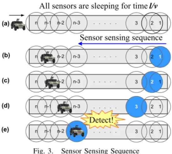
Based on the fact that targets move only along the roadways, we propose a new design called Virtual Scanning. As shown in Figure 3, after all sensors sleep forl/vseconds, we turn on sensors one by one for working time w from the rightmost sensor s1 toward the leftmost onesn. Clearly, this wave of sensing activities
n . . . . . (b)
Sensor sensing sequence
n-1 n-2 n-3 3 2 1 n . . . . . (c) n-1 n-2 n-3 3 2 n . . . . . (d) n-1 n-2 n-3 3 1 n . . . . . (e) n-1 n-3 3 2 1 n . . . . . (a)
All sensors are sleeping for timel/v
n-1 n-2 n-3 3 2 1
1
2
n-2
Detect!
Fig. 3. Sensor Sensing Sequence
guarantees the detection and allows additional sleeping time for individual sensors. Compared with Duty Cycling, this additional sleeping time is obtained by the fact thatall sensors but one can sleep during the scan. We note that the direction of a virtual scan shall be from the protection point to the entrance point. The virtual scan of the opposite direction (i.e., from the entrance point to the protection point) cannot guarantee target intrusion detection, if a very fast target enters right after the beginning of the network-wide silent time.
B. Analytical Network Lifetime Comparison
To understand key design parameters, this section compares analytically the network lifetime among the Always-Awake,Duty CyclingandVirtual Scanningmethods. For clarity, we summarize the notation in Table I and overall analytical results in Table II.
TABLE I
NOTATION OFPARAMETERS FORANALYSIS Parameter Definition
Tlif e Lifetime that a sensor can work continuously
corresponding to its energy budget.
Tnet Sensor network lifetime.
Twork Working time that a sensor needs to work for
reliable detection. NormallyTwork=w.
Tsleep Sleeping time of each sensor.
Tscan Scan time that a virtual scan wave moves along
the road segment.Tscan=nw.
Tsilent Silent time that the whole sensor network remains
silent; that is, time that a target passes through the road segment of lengthl.Tsilent=l/v.
Tperiod Schedule period of the sensor network.
Tperiod=Tscan+Tsilent.
Always-Awake & Duty Cycling: For the Always-Awake ap-proach, the network lifetime Tnet is the same as Tlif e, because
sensors work continuously without sleeping. For theDuty Cycling
approach, the network lifetime Tnet is the number of periods
Tlife
w multiplied by the length of the period Tperiod (i.e., the
sum of the silent time vl and the working timew):
Tnet=Tlif e
w ( l
v +w) (1)
Virtual Scanning: In the Virtual Scanning, the network lifetime
Tnet is the number of periods Tlifew multiplied by the period
length Tperiod.Tperiod is the sum of the scan timenwand silent
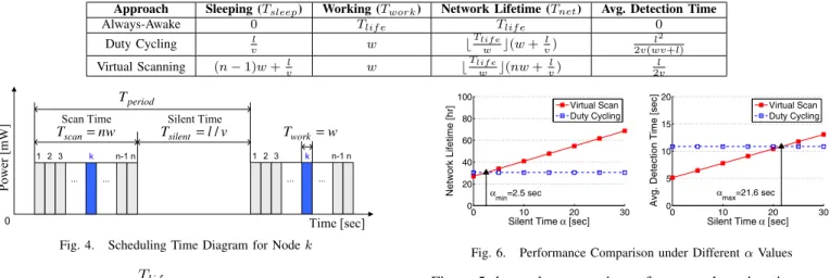
TABLE II
PERFORMANCEANALYSIS FORTHREEAPPROACHES
Approach Sleeping (Tsleep) Working (Twork) Network Lifetime (Tnet) Avg. Detection Time
Always-Awake 0 Tlif e Tlif e 0
Duty Cycling l v w Tlife w (w+vl) l 2 2v(wv+l) Virtual Scanning (n−1)w+ l v w Tlife w (nw+vl) 2lv 1 23 k n-1 n ... ... Time [sec] 0 Power [mW] w Twork= period T 1 23 k n-1 n ... ... nw Tscan= Tsilent=l/v Scan Time Silent Time
Fig. 4. Scheduling Time Diagram for Nodek
Tnet=Tlif e w (Tscan+Tsilent) =Tlif e w (nw+ l v) (2)
Figure 5 shows the comparison of lifetime among these three approaches. For example, forw= 1sec,Virtual Scanninghas the lifetime of 30 hours, Duty Cycling3.2 hours, and Always-Awake
0.14 hour;Virtual Scanninghas 9.4 times lifetime ofDuty Cycling
and 214 times lifetime of Always-Awake.
0 1 2 3 4 5 0 5 10 15 20
Working Time w [sec]
Avg. Detection Time [sec]
Virtual Scan Duty Cycling Always−Awake 0 1 2 3 4 5 0 20 40 60
Working Time w [sec]
Network Lifetime [hr]
Virtual Scan Duty Cycling Always−Awake
Fig. 5. Performance Comparison according to Working Timew C. Analytical Detection Time Comparison
This section compares the average detection time after a target entering a road segment among the Always-Awake,Duty Cycling
andVirtual Scanningmethods.
Always-Awake & Duty Cycling: For Always-Awake, since a target is detected as soon as it enters the road segment, the average detection time is zero. For the Duty Cycling, if a target enters during the working period, detection time is zero. On the other hand, if a target enters during the silent time, average detection time is half of the silent time l/(2v). The percentage of silent time within a period isl/(wv+l), therefore, the overall average detection time of theDuty Cyclingapproach isl2/(2v(wv+l)). Virtual Scanning: We suppose thatnsensors are deployed on a road segment, so each sensor covers the length ofl/nin average. Also, we suppose that target speed is v and a target can arrive at any time; that is, the arrival time is uniformly distributed. A target can arrive either duringscan timeorsilent time. We analyze separately the average detection time for each period and then combine them to obtain overall expected delayl/(2v). Please refer to our extended technical report [5] for detailed derivation; note that the average detection time for bounded variable target speed is also derived. 0 10 20 30 0 5 10 15 20
Silent Time α [sec]
Avg. Detection Time [sec]
Virtual Scan Duty Cycling 0 10 20 30 0 20 40 60 80 100
Silent Time α [sec]
Network Lifetime [hr]
Virtual Scan Duty Cycling
αmin=2.5 sec αmax=21.6 sec
Fig. 6. Performance Comparison under DifferentαValues
Figure 5 shows the comparison of average detection time among the three approaches. Virtual Scanning detects with a constant delay l/(2v) regardless of working time w. On the other hand, the average detection time of the Duty Cycling tends to de-crease slowly while working timewincreases. TheAlways-Awake
method detects without any delay. For example, for working time
w = 0.1 sec, Virtual Scanning has similar performance with
Duty Cycling, about 10.9 sec. For working time w = 5sec, the
Virtual Scanningdetects target within 10.9 sec in average and the
Duty Cycling does within 8.87 sec; the average detection delay ratio between theVirtual Scanning and theDuty Cyclingis 1.23. However, the ratio of the Virtual Scanning’s network lifetime to the Duty Cycling’s network lifetime is 37, as shown in Figure 5. Thus, even though the average detection time increases slightly with Virtual Scanning, the benefit of network lifetime is quite remarkable.
D. Configuring VISA for Better Delay and Longer Lifetime
As a reminder, when the network silent time Tsilent is equal
to or smaller thanl/v, target detection is guaranteed. Basic VISA design uses l/v as the network silent time Tsilent. However, if a
smaller silent timeTsilentis used, it is possible to detect the target
not only faster but also with less energy than the Duty Cycling
algorithm.
Let Tsilent =α forα∈[0,l/v]. In order to outperformDuty
Cycling in both network lifetime and average detection delay, we shall satisfy the following inequalities:
Virtual Scanning Duty Cycling Tlife w (nw+α) ≥ Tlife w (w+vl) l(nw+α) 2(nwv+l) ≤ l 2 2v(wv+l) (3)
Solving the above inequalities, we have:
max{l v −(n−1)w,0} ≤α≤min{ l(nwv+l) v(wv+l) −nw, l v}
When α falls into this range, Virtual Scanning has better performance thanDuty Cyclingin both the average detection time and network lifetime. For example, as shown in Figure 6, for
w= 0.1 sec, whenαis less than αmax= 21.6 sec, the average
detection time of Virtual Scanning is shorter than that of Duty Cycling. Also, when α is greater than αmin = 2.5 sec, Virtual Scanning’s lifetime is longer thanDuty Cycling’s. Thus, the range
of αachieving better detection delay and lifetime is [2.5, 21.6] sec. We note the results here only illustrate the idea. Detailed study on the performance effect of α is presented in evaluation Section IV-B3.
III. VIRTUALSCANNINGALGORITHMSYSTEMDESIGN For the sake of clarity, the previous section presents the basic idea using one road segment. In the rest of the paper, we demonstrate how to apply the virtual scanning to road networks with arbitrary topology. This section is organized as follows: Section III-A lists definitions and assumptions used in VISA. Section III-B describes the scheduling algorithm, and Section III-C presents the hole handling algorithm.
A. Definitions and Assumptions
Definition 3.1 (Road Network Graph): Let Road Network Graph be G = (V, E), where V = {v1, v2, ..., vn} is a set of
intersections, entrance points, and protection points in the road network under surveillance, and E = [eij] is a matrix of road
segment lengtheij for verticesviandvj. Figure 7 shows a graph Gcorresponding to the road network in Figure 1.
1 9 2 10 3 11 14 15 12 13 5 6 7 18 8 16 17 4 200 80 200 150 140 130 70 100 250 110 170 100 140 180 160 150 140 110 140 270 150 250 140 80 E E E E P P P P
s
G
Fig. 7. Road Network GraphG
Definition 3.2 (Network Lifetime): LetNetwork Lifetimebe the duration from the starting of a sensor network for surveillance until a target can possibly reach one of the protection points without detection. In other words, lifetime ends when there exists a possible breach path between an entrance point to a protection point.
Definition 3.3 (VISA Scheduler): LetVISA Schedulerbe a sink node that initiates the sensing scheduling algorithm.
The VISA design is based on the following assumptions:
• Road map and locations of sensor nodes are known to
VISA Scheduler. The sensor location can be obtained through localization schemes [6].
• Sensors are roughly time-synchronized at tens of millisecond level. It can be easily achieved because existing solutions [7], [8] can achieve microsecond level accuracy.
• Sensors only have simple sensing devices for binary target detection, such as PIR sensors [9]. No sophisticated hardware is available.
• One of existing low-duty-cycle data forwarding schemes, such as DSF [10] and DESS [11] is used to deliver nodes’ locations and target detection results to the VISA scheduler.
• Targets move only along predefined roads with the bounded maximum speed.
B. VISA Scheduling on Road Network
This section presents the design of virtual scanning, including schedule establishment and dissemination.
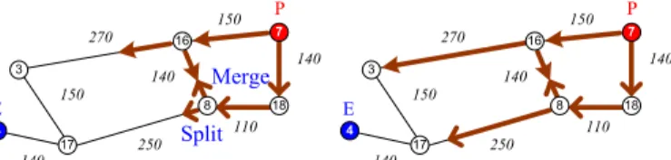
1) Establishment of Working Schedule: For clarity in presenta-tion, we use the subgraph Gs of the graphGshown in Figure 7
where the edge weight means the physical distance of the road segment. First, we will consider a road network with one entrance and one protection point at first, and then will consider a road network with multiple entrances and multiple protection points. Also, for now, we assume that no sensing holes exist in the middle of roadways where targets cannot be detected due to the non-existence of sensors. The sensing hole handling will be discussed in Section III-C. E P 3 8 16 17 4 Split 150 140 110 140 270 150 250 140 7 18
(a) Virtual scan originates from protec-tion pointv7and splits into two scans
150 140 110 140 270 150 250 140 E P Split 3 7 18 8 16 17 4
(b) Virtual scan arriving at v16 splits into two scans towardsv3andv8 150 140 110 140 270 150 250 140 E P Merge Split 3 7 16 17 4 8 18
(c) Two scans fromv8 andv16merge at the road segment(v8, v16)and stop
150 140 110 140 270 150 250 140 E P 3 7 16 17 4 8 18
(d) Two scans keep going towards in-tersectionsv3andv17, respectively
150 140 110 140 270 150 250 140 E P Merge Split 3 7 18 16 17 4 8
(e) Two scans fromv3 andv17merge at the road segment(v3, v17)and stop
150 140 110 140 270 150 250 140 E P 3 7 18 16 17 4 8
(f) Virtual scan finally arrives at en-trance pointv4and the scan is done Fig. 8. Virtual Scanning on Road Network for Working Schedule Establishment
Figure 8 shows the snapshots of virtual scanning in the road networkGswith one entrancev4labeled asEand one protection
pointv7labeled asP. The virtual scan’s propagation time on each road segment is the multiplication of the number of sensors and the individual working time w, instead of the physical distance of a road segment. As shown in Figure 8, by turning on sensors along roads consecutively, virtual scanning waves propagate along multiple routes simultaneously, split at intersections, and disappear when two waves encounter each other in a road segment.
In the case of multiple entrance and protection points, scan operation is similar, except that multiple protection points initiate scanning at the same time. Because the waves merge in the middle of road segments during virtual scanning (as shown in Figure 8(c)), regardless the number of protection points and the locations of the sensors, each sensor only works forwseconds per scan, which is a nice feature for energy balance. Clearly, the scan wave arrival time for each sensor can be easily computed with All-Pairs Shortest Path algorithm, such as Floyd-Warshall algorithm [12]. We note the scan wave arrival time decides the working schedule of a
sensor node. In other words, a sensor shall start to work for w
seconds after a virtual scanning wave arrives.
2) Decentralized Implementation: In a centralized implemen-tation, a VISA scheduler calculates the work schedules for all sensors and disseminate the results, which leads to far more messages than necessary ones. Actually the scan wave arrival time for each sensor can be calculated in a decentralized way. During the initialization phase, all sensors are awake. The sensors at the protection points generate short messages containing a counter with value initialized to one, and pass them to their immediate neighboring sensors. The neighboring sensors only record the minimum counter value ever seen (i.e., discard the rest of messages arriving late), increment the counter, and then relay the message to their neighboring sensors. If a sensor is located at a road intersection, it duplicates and relays multiple copies of messages to all its neighboring nodes except the one it received the message from. In this way, the sensors can decide their sensing scanning order (i.e., the minimum counter value) in the distributed way. Given a sensing order of K, a node shall start to work at timeKw and stop at time(K+ 1)w.
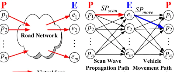
Road Network Virtual Scan 1 p 2 p n p . . . 1 e 2 e m e . . .
P
E
(a) Virtual Scanning on an Arbi-trary Road Network with Protec-tion Points and Entrance Points
1 p 2 p n p 1 e 2 e m e
P
E
. . . . . . . . . Scan Wave Propagation Path Vehicle Movement Path scan SP move SPP
1 p 2 p n p(b) Sleeping Time Computation considering the Shortest Scanning and Movement Paths
Fig. 9. Virtual Scanning on Road Networks
3) Establishment of Sleeping Schedule: The previous section discussed how to decide working schedule during the scan. This section explains how to compute the optimal sleeping length, i.e., the maximum duration sensors can sleep safely after working for
wseconds while guaranteeing the detection.
Figure 9(a) shows the virtual scanning in an arbitrary road network. Let P = {p1, ..., pn} be the set of protection points.
LetE ={e1, ..., em} be the set of entrance points. As discussed
before, a period Tperiod consists of (i) silent timeTsilent during
which the whole network is turned off and (ii) scan time Tscan
during which scan waves propagate across the network. Since a sensor only works for fixedTwork=wseconds everyTperiod, the
longerTperiodis, the better energy efficiency we have. Therefore,
we shall identify the maximum Tperiod value that can guarantee
the detection. Before this optimization, we define two important concepts as below:
Definition 3.4 (The Shortest Scanning Path): The Shortest Scanning Path pscan(i, j) is the shortest-delay path for wave propagation from vi to vj on the graph G, where vi ∈ P and vj ∈E. Let lscan(i, j)be the number of sensors along the path
pscan(i, j). Therefore, the Shortest Scanning Time Tscan(i, j)
can be computed aslscan(i, j)∗w.
Definition 3.5 (The Shortest Movement Path): The Shortest Movement Pathpmove(i, j)is the shortest-distance path between
vertices vi and vj on the graph G where vi ∈ E and vj ∈ P.
Let lmove(i, j)be the shortest distance ofpmove(i, j). Therefore,
the Shortest Movement Time Tsilent(i, j) can be computed as
lmove(i, j)/vmax, where vmax is maximum target speed. We
note that all of the sensors along the path pmove(i, j) can sleep together for the silent timeTsilent(i, j).
These two shortest pathspscan(i, j)andpmove(i, j)for all pairs of vertices can be computed based onGby the All-Pairs Shortest Paths algorithm, such asFloyd-Warshall algorithm.
An important principle of computing the optimal sleeping time is that all of vehicles entering during the sleeping time must be detected before their arrival to the protection points. Once a virtual scan wave originating from the protection points has swept an entrance point, the paths from this swept entrance point to the protection points are vulnerable to the target intrusion. This is because the swept paths are not swept again until the next scan period.
It is noted that we can guarantee detection by setting Tperiod
as the sum of all-pair minimum scanning time and all-pair minimum movement time. However, the resulting Tperiod is
shorter than the optimal value, (i) because an intruding target could have to travel a longer route from an entrance point with theearliestscan arriving time thanall-pair minimum movement time, or (ii) because it could have to wait until a late scan arrives before it can travel along the shortest route with all-pair minimum movement time, especially when sensors are non-uniformly placed across a network. Therefore, the optimal safe
Tperiodshall be theminimum sumof thescanning timefromvi
tovjand thevehicle movement timefromvjtovk, forvi, vk∈P
andvj ∈E.
Figure 9(b) shows a three-column graph for computing the period Tperiod. The edges between the first and second columns
denote the time for wave propagation and the edges between the second and third columns denote the time for target movement. To compute a safe and optimalTperiod, we need to identify the
short-est path from any vertex in the first column to any vertex in the third column. Without loss of generality, supposep1⇒e1⇒p2is the shortest path. Once the virtual scan arrives at the entrance point
e1 with a delay ofTscan(p1, e1), the path from the entrance point e1 to the protection pointp2 becomes vulnerable, if the network remains silent for more than Tsilent(e1, p2). Thus, to prevent a target from reaching the protection point p2 without detection, another scan wave must be generated from the protection point
p2 after Tsilent(e1, p2). Therefore, the safe and optimal period
is Tperiod = Tscan(p1, e1) +Tsilent(e1, p2). Consequently, the
sleeping time is Tsleep =Tperiod−Twork, because each sensor
must work for its duty cycle Twork=wseconds per period.
Now, we can formally define the optimization problem of the sleeping time. Let Tsleep(i, j, k) = Tscan(i, j) +Tsilent(j, k)− Twork for vi, vk∈P andvj∈E where Twork =w. The optimal
sleeping time is chosen as follows:
Tsleep← min
vi,vk∈P,
vj∈E
Tsleep(i, j, k).
(4) Obviously, the searching for an optimal sleeping time is done in polynomial time O(mn2). Once the sleeping time value is computed byVISA scheduler, it piggybacks in the counter message
1 2 3 4 4 1 2 2 3 4
Sensing Hole Segment
5 H H4 1 H 2 H 3 H
(a) Sensing Hole Segments on Road Network:Hi= (hj, hk) 1 v 2 v v10 11 v 9 v 12 v 13 v v5 6 v 15 v 14 v 16 v v7 18 v 8 v 3 v 17 v 4 v E E E P P P P E 9 h 10 h 7 h 8 h 2 h 1 h 4 h 3 h 5 h h6 i P
(b) Augmented Graph including Sens-ing Holes:Ga= (Va, Ea)
Fig. 10. Augmentation of Road Network Graph with Sensing Holes discussed in Section III-B2 and is disseminated to all the sensors in the network. If the VISA scheduler changes the locations of protection and entrance points dynamically, it only needs to re-calculate a new sleeping time and re-disseminate it.
Till now, the sensors know when to wake up in order to create virtual scanning (i.e., Working Schedule in Section III-B1) and how long they can safely sleep with optimal efficiency (i.e., Sleeping Schedule in Section III-B3).
C. Handling of Sensing Holes
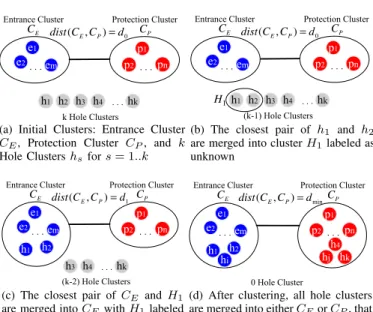
We have so far discussed the sensor working schedule and sleeping schedule, assuming balanced energy and no initial sensing holes. In this section, we discuss the handling of sensing holes that can exist after the sensor deployment and that can occur due to sensor failure or energy depletion. As shown in Figure 10(a), five sensing hole segments (i.e.,H1,...,H5) exist in the given road network graph. Our idea to deal with these initial hole segments is that we make an augmented graph by adding the endpoints of the hole segments as shown in Figure 10(b). To ensure the protection, we treat these endpoints as eitherpseudoentrance points orpseudo
protection points. The hole handling problem is, therefore, reduced to a labeling problem of hole segment endpoints.
Problem Definition: How to optimally determine the role of each hole endpoint (i.e., label as either entrance point or protection point) in order to achieve the maximum sleeping time, leading to the maximization of the sensor network lifetime.
In the rest of this section, we present an optimal labeling algorithm for hole handling.
1) Initial Sensing Holes: In reality, there is high probability that some road segments are not covered by sensors even though many sensors are randomly deployed on road network as shown in Figure 10(a). We define these uncovered road segments as the
initial sensing hole segments; note that each sensing hole segment consists of two hole endpoints.
Suppose that n hole endpoints occur under a uniform sensor density. With an exhaustive search, 2n cases are required to investigate. This means the time complexity ofO(2n). Since this
complexity is intractable, we need an improved way to achieve an optimal labeling for hole endpoints.
We explain here the idea with a simplified example; Fig-ure 10(b) shows one roadway Pi consisting of v3, v16, and v7
and a hole segmentH1with hole endpointsh1andh2, which are closer to a protection point v7 than an entrance point v3. If two hole endpoints h1 and h2 are labeled differently, this short hole
segment determines the shortest sleeping time. To avoid this, h1 and h2 should have the same type of label. Furthermore, since h1 andh2 near the protection point v7, in order to get a longer sleeping time, they should be labeled as protection points.
Conceptually, when labeling hole endpoints, we should label each hole endpoint with the same label as the closest point already labeled. Rationale behind this insight is: the maximization of the path distance between the entrance points and protection points leads to a maximum sleeping time according to Eq. 4.
Formally, let H be the set of hole endpoints such that H = {h1, h2, . . . , hk}. LetEbe the set of entrance points andP be the
set of protection points. LetLE be entrance label andLP be
pro-tection label. We can label the holes inH, by partitioningH into two disjoint subsets (called clusters) Entrance Cluster (CE) and
Protection Cluster (CP). Asano et al. proposed such a clustering
algorithm for a farthest k-partition based on Minimum Spanning Tree (MST) [13], giving an optimal clustering to maximize the inter-cluster distance. We extend Asano’s Clustering for sensing hole labeling. p2 e2 p1 pn . . . e1 em . . . h2 . . .hk k Hole Clusters 0 ) , (C C d dist E P = h3 h4
Entrance Cluster Protection Cluster
E
C CP
h1
(a) Initial Clusters: Entrance Cluster
CE, Protection Cluster CP, and k
Hole Clustershsfors= 1..k
(k-1) Hole Clusters e1 e2. . .em p1 p2 . . .pn 0 ) , (C C d dist E P =
Entrance Cluster Protection Cluster
E C CP h2 h3 h4 . . .hk h1 1 H
(b) The closest pair of h1 and h2
are merged into clusterH1labeled as unknown e1 e2 em . . . h1 h2 1 ) , (C C d dist E P =
Entrance Cluster Protection Cluster E C CP p1 p2 . . . pn hk . . . (k-2) Hole Clusters h3 h4
(c) The closest pair ofCE andH1
are merged intoCEwithH1labeled as entrance labelLE e1 e2 em . . . p1 p2 . . .pn h1 h2 0 Hole Cluster min ) , (C C d dist E P = h4 hi hj hk
Entrance Cluster Protection Cluster E
C CP
(d) After clustering, all hole clusters are merged into eitherCEorCP, that is, labeled as eitherLE orLP
Fig. 11. Clustering for Sensing Hole Labeling
Figure 11 illustrates the main idea. Let dist(CE, CP) be the
inter-cluster distance between CE and CP. Our objective is to
partition the set H into two disjoint sets CE and CP such that
the inter-cluster distance betweenCE andCP is maximized. The
initial inter-cluster distance is dist(CE, CP) =d0, as shown in Figure 11(a). In this example, suppose that two hole clusters h1 and h2 are the closest pair of two clusters. In this case, these hole clusters are merged into one hole clusterH1with the same, unknown label, as shown in Figure 11(b). The reason two clusters
h1andh2are merged into one hole cluster with the same label is to let the inter-cluster distance betweenCEandCP be maximized.
Otherwise, the inter-cluster distance betweenh1andh2can be the inter-cluster distance shorter than the initial inter-cluster distance
dist(CE, CP) =d0. As shown in Figure 11(c), two clusters CE
and H1 are the closest pair, so H1 is merged into CE with hole
endpoints h1 and h2 labeled as entrance. In this way, we can cluster all of the hole endpoints into eitherCEorCP to maximize
Similar to Asano’s algorithm [13], our clustering gives an optimal hole labeling because it satisfies the greedy choice propertyand
optimal substructure[12].
As an important difference from Asano’s Clustering, during the clustering, we maintain multiple hole clusters Hi labeled
as unknown in addition to one Entrance Cluster CE and one
Protection ClusterCP. Through the MST construction, we merge
one hole clusterHi to eitherCEorCP such that the inter-cluster
distance between CE and CP is maximized. We call this new
labeling algorithm theMST-based Labeling.
2) Sensing Holes due to Energy Depletion or Failure: In the previous section, we discussed the initial sensing hole issue. However, since in reality, the sensors deployed on road network may not have the same amount of energy initially, we need to consider the sensing holes caused by this unbalanced sensor energy budget. Also sensor could fail over time. We can deal with these sensing holes in the same way as with the initial holes; we can either completely relabel all holes or incrementally label new holes by usingMST-based Labeling. The former is optimal, but the latter introduces less computation.
3) Other Practical Issues: We have considered three practical issues in our extended technical report [5] for the deployment of our surveillance scheme in real road networks: (i) detection-error probability, (ii) time synchronization detection-error, and (iii) commu-nication design for detection report. These issues are out of the main scope of this paper, hence we omit them here due to space constraints.
IV. PERFORMANCEEVALUATION
In this section, we analyze performance of VISA, comparing with other schemes for road network surveillance.
• Performance Metrics:We usenetwork lifetimeandaverage detection timeas the performance metrics.
• Baselines: Since the road network surveillance is a new research area, to the best of our knowledge, there exist no other state-of-the-art sensing schemes for road network surveillance. We compare VISA with two approaches: Duty Cycling andAlways-Awake.
• Parameters:In the performance comparison, we investigate the effect of the following three parameters: (i) working time, (ii) sensor density, and (iii) energy budget. In addition, we reveal (i) the effect of sleeping time duration and (ii) the effect of sensing hole labeling.
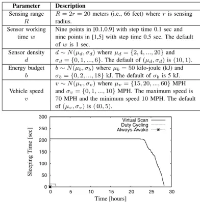
Simulation uses the map of a real road network as shown in Figure 7. The system parameters are selected based on a typical military scenario [14]. Unless mentioned otherwise, the default values in Table III are used.
For network lifetime measurement, the default energy budget (50 kJ) is used, but for the average detection time measurement, to obtain high statistical confidence, a full-day energy budget is used for the comparison among the three approaches. The vehicle arrival time is uniformly distributed during the system lifetime with mean inter-arrival time 60 sec.
A. System Behavior over Time
All three methodsVirtual Scanning,Duty Cyclingand Always-Awakecan guarantee the detection of targets. Their difference lies
TABLE III SIMULATIONCONFIGURATION Parameter Description
Sensing range R= 2r= 20meters (i.e., 66 feet) whereris sensing
R radius.
Sensor working Nine points in [0.1,0.9] with step time 0.1 sec and timew nine points in [1,5] with step time 0.5 sec. The default
ofwis 1 sec.
Sensor density d∼N(μd, σd)whereμd={2,4, ...,20}and
d σd={0,1, ...,6}. The default of(μd, σd)is(10,1). Energy budget b∼N(μb, σb)whereμb= 50kilo-joule (kJ) and
b σb={0,2, ...,18}kJ. The default ofσbis 5 kJ.
v∼N(μv, σv)whereμv={15,20, ...,60}MPH Vehicle speed andσv={0,1, ...,10}MPH. The maximum speed is
v 70MPH and the minimum speed10MPH. The default of(μv, σv)is(40,5). 0 50 100 150 200 250 300 0 5 10 15 20 25 30
Sleeping Time [sec]
Time [hours]
Virtual Scan Duty Cycling Always-Awake
Fig. 12. Comparison of Sleeping TimeTsleepover Time
in the network lifetime. Clearly, the longer a node can sleep safely per period, the more energy efficiency is. Figure 12 shows how the sleeping time Tsleep changes before network lifetime ends.
As shown in the figure, Virtual Scanning has by far the longest sleeping time and hence the longest network lifetime. For example,
Virtual Scanningsustains for 28.2 hours, compared with 1.4 hours inDuty Cyclingand 5.4 minutes inAlways-Awake. This is because of the significant energy saving during the scanning process.
B. Performance Comparison
In this section, we compare three approaches: (i) Virtual Scan-ning, (ii)Duty Cyclingand (iii)Always-Awakein terms of Network Lifetime and Average Detection Time under several user-level parameters, such as working time duration, energy budget, and sensor density. Each point in each experiment is the mean of the results obtained with 10 different random seeds.
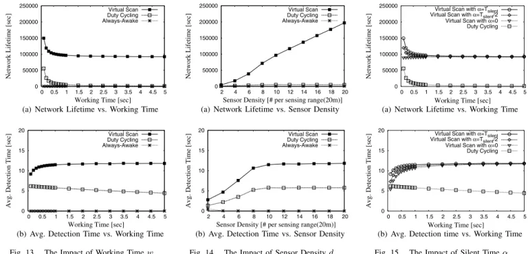
1) The Impact of Working Time: Since w is the minimum working time before reliable detection can be reported, this evaluation reveals how different hardware response speeds and sensing algorithms affect the VISA and other baselines. We use non-uniform50kJ energy budget with the energy variation5kJ. Clearly, VISA provides significantly longer system lifetime than the baselines, especially whenwis large as shown in Figure 13(a). For example, whenwis 1 second, VISA extends network lifetime by 18.5 times, compared with Duty Cycling and 146 times, compared withAlways-Awake. As shown Figure 13(b), the average detection time of Virtual Scanning is 11.5 sec, which is two times longer than that ofDuty Cycling, 5.8 sec. Therefore,Virtual Scanning can provide 19 times lifetime of Duty Cycling at the expense of two times longer average detection time.
2) The Impact of Sensor Density: We define sensor density
0 50000 100000 150000 200000 250000 0 0.5 1 1.5 2 2.5 3 3.5 4 4.5 5
Network Lifetime [sec]
Working Time [sec]
Virtual Scan Duty Cycling Always-Awake
(a) Network Lifetime vs. Working Time
0 5 10 15 20 0 0.5 1 1.5 2 2.5 3 3.5 4 4.5 5
Avg. Detection Time [sec]
Working Time [sec]
Virtual Scan Duty Cycling Always-Awake
(b) Avg. Detection Time vs. Working Time Fig. 13. The Impact of Working Timew
0 50000 100000 150000 200000 250000 2 4 6 8 10 12 14 16 18 20
Network Lifetime [sec]
Sensor Density [# per sensing range(20m)]
Virtual Scan Duty Cycling Always-Awake
(a) Network Lifetime vs. Sensor Density
0 5 10 15 20 2 4 6 8 10 12 14 16 18 20
Avg. Detection Time [sec]
Sensor Density [# per sensing range(20m)]
Virtual Scan Duty Cycling Always-Awake
(b) Avg. Detection Time vs. Sensor Density Fig. 14. The Impact of Sensor Densityd
0 50000 100000 150000 200000 250000 0 0.5 1 1.5 2 2.5 3 3.5 4 4.5 5
Network Lifetime [sec]
Working Time [sec]
Virtual Scan with α=Tsilent
Virtual Scan with α=Tsilent/2
Virtual Scan with α=0 Duty Cycling
(a) Network Lifetime vs. Working Time
0 5 10 15 20 0 0.5 1 1.5 2 2.5 3 3.5 4 4.5 5
Avg. Detection Time [sec]
Working Time [sec]
Virtual Scan with α=Tsilent Virtual Scan with α=Tsilent/2 Virtual Scan with α=0 Duty Cycling
(b) Avg. Detection time vs. Working Time Fig. 15. The Impact of Silent Timeα
expected from the formula of the network lifetime in Eq. 2, the high sensor density provides the longer network lifetime for
Virtual Scanning. This is because with a higher density, we have a longer scanning timeTscan, which allows sensor nodes to sleep
longer. However, the high sensor density does not contribute much to the network lifetime toDuty CyclingandAlways-Awake, since their sleeping time is independent of the number of sensors (as shown in Table II). For the average detection time, in bothVirtual ScanningandDuty Cycling, e.g., under sparse sensor density less than 8, the lower density lets the sensors close to entrances detect vehicles earlier. This is because many sensor network clusters occur due to initial sensing holes, so the sleeping time becomes short. Thus, the sensors close to entrances wake up early and detect targets, leading to shorter detection time. In summary, at all sensor density settings, Virtual Scanning provides the longest network lifetime with a slight increase in detection time; note that the performance gain of Virtual Scanning becomes higher when sensor density becomes higher.
3) Achieving Shorter Delay and Longer Lifetime Simulta-neously: In Section II-D, we showed analytically how VISA achieves a shorter delay and a longer network lifetime simultane-ously by adjusting the silent time(Tsilent=α) within the range
that satisfies Eq. 3. To confirm our design empirically, Figure 15 shows the performance effect of Virtual Scanning according to
α. As shown in Figure 15, when Virtual Scanning reduces α
fromTsilent to0in the working time of0.1 second, it has better
performance in both the network lifetime and average detection time thanDuty Cycling.
C. The Effect of Hole Handling
This section compares three different methods for hole handling as follows:
• MST-based Labeling: our hole labeling scheme discussed in Section III-C.
• Random Labeling: a new hole is randomly labeled as either
pseudo entrance point orpseudo protection point.
• No Labeling: when a new hole occurs, it is not handled, leading to the end of system lifetime.
0 50000 100000 150000 200000 250000 0 0.5 1 1.5 2 2.5 3 3.5 4 4.5 5
Network Lifetime [sec]
Working Time [sec]
MST-based Labeling Random Labeling No Labeling
Fig. 16. Performance Comparison of Hole Labeling Algorithms We use the same Virtual Scanning for these three labeling algorithms. As shown in Figure 16, MST-based Labeling gives longer lifetime than both Random Labeling and No Labeling.
Random Labeling and No Labeling have the similar lifetime, because Random Labeling cannot label holes appropriately to prevent a breach path (i.e., path vulnerable to vehicle intrusion to protection points) from existing. Since No Labeling does not handle sensing hole, one sensing hole creates a breach path, leading to the end of system. For the average detection time, these three labeling algorithms have similar performance whose curves are almost the same as the curve of Virtual Scanning in Figure 13(b).
V. RELATEDWORK
Most research on coverage for detection has so far focused on Full Coverage[1]–[4], [15]–[18] in a two-dimensional space. In [4], authors use the off-duty eligibility rule to turn on/off a node as long as the neighboring nodes can cover the sensing area of this node. The Coverage Configuration Protocol (CCP) [16] provides an energy-efficient sensing coverage, integrated with SPAN for connectivity. In [19], surveillance coverage is achieved through
probing. DiffSurv [20] provides differentiated surveillance to an area with a certain degree of coverage, up to the limitation imposed by the number of sensor nodes deployed. Kumar et al. [3] identify a critical bound for k-coverage in a network, assuming a node is randomly turned on with a certain probability. In [2], Cardei et al. propose two heuristic algorithms to identify a maximum number of set covers to monitor a set of static targets at known locations. In [1], Abrams et al. propose three approximation algorithms for a relaxed version of the previously defined SET K-COVER problem [21].
To aggressively reduce energy consumption, partial coverage through Duty Cycling has been studied as well. In [22], [23], authors provide a theoretical analysis and simulation on the delay (or stealth distance) before a target is detected. In [22], the Quality of Surveillance (QoSv) is defined as the reciprocal value of the expected travel distance before mobile targets are first detected by any sensor. In [24], nodes coordinate among each other to guarantee the worst-case detection delay and minimize the average detection delay. In [25]–[27], the theoretical foundations for laying barriers with stealthy and wireless sensors are proposed in order to detect the intrusion of mobile targets approaching the barriers from the outside.
The closest related work isvirtual patrol[28], in which avirtual patrolmoves along the predefined path in 2-dimensional space and triggers sensors adjacent to the virtual patrol’s path for detection. This virtual patrol is similar to the concept of our virtual scan. However, the uniqueness of our work can be clearly identified from the following respects: (i) our work focuses on surveillance in road network, where legacy two-dimensional solutions cannot directly apply, and (ii) we are the first to formally guarantee target detection while sensor network deteriorates, using a hole handling technique.
VI. CONCLUSION
Specially tailored for road networks, this work introducesVISA
based on the concept of virtual scanning.VISApropagates sensing waves along the roadways and detects vehicles entering into the target road network before they reach the protection points. We demonstrate analytically and empirically the feasibility of achieving longer network lifetime and shorter detection delay simultaneously. In addition, we propose an optimal algorithm to deal with the initial sensing holes at the deployment time as well as the sensing holes due to node failure and the heterogeneous energy budget among sensors by optimally labeling additional
pseudoprotection or entrance points. Evaluation shows orders-of-magnitude longer network lifetime than the always-awake method, and as much as ten times longer than the duty cycling algorithms. We believe this work opens a promising direction of road network surveillance. Future work includes (i) the perimeter protection of road networks, (ii) protection design with bounded detection delay, (iii) optimal sensor placement with minimal detection delay, and (iv) extension for civil applications, such as corridor surveillance and water pipeline inspection.
ACKNOWLEDGMENT
This research was supported by the Digital Technology Center at the University of Minnesota, and in part by NSF grants CNS-0626609, CNS-0626614, and CNS-0720465.
REFERENCES
[1] Z. Abrams, A. Goel, and S. Plotkin, “Set K-Cover Algorithms for Energy Efficient Monitoring in Wireless Sensor Networks,” inIPSN. ACM/IEEE, 2004.
[2] M. Cardei, M. T. Thai, Y. Li, and W. Wu, “Energy-Efficient Target Coverage in Wireless Sensor Networks,” inIEEE. INFOCOM, 2005.
[3] S. Kumar, T. H. Lai, and J. Balogh., “On K-Coverage in a Mostly Sleeping Sensor Network,” inMOBICOM. ACM, 2004.
[4] D. Tian and N. Georganas, “A Node Scheduling Scheme for Energy Conser-vation in Large Wireless Sensor Networks,”Wireless Communications and Mobile Computing Journal, May 2003.
[5] J. Jeong, Y. Gu, T. He, and D. Du, “VISA: Virtual Scanning Algorithm for Dynamic Protection of Road Networks,” Tech. Rep. 08-026, Aug. 2008, http://www.cs.umn.edu/research/technical reports.php? page=report&report id=08-026.
[6] A. Savvides, C. C. Han, and M. B. Srivastava, “Dynamic Fine-Grained Localization in Ad-Hoc Networks of Sensors,” inMOBICOM. Rome, Italy: ACM, Jul. 2001.
[7] J. Elson, L. Girod, and D. Estrin, “Fine-Grained Network Time Synchroniza-tion using Reference Broadcasts,” inOSDI. ACM, Dec. 2002.
[8] M. Mar´oti, B. Kusy, G. Simon, and ´Akos L´edeczi, “The Flooding Time Synchronization Protocol,” inSENSYS. Baltimore, Maryland, USA: ACM, Nov. 2004.
[9] Lin Gu et al., “Lightweight Detection and Classification for Wireless Sensor Networks in Realistic Environments,” inSENSYS. San Diego, California, USA: ACM, Nov. 2005.
[10] Y. Gu and T. He, “Data Forwarding in Extremely Low Duty-Cycle Sensor Networks with Unreliable Communication Links,” in SENSYS. Sydney, Australia: ACM, Nov. 2007, pp. 321–334.
[11] G. Lu, N. Sadagopan, B. Krishnamachari, and A. Goel, “Delay Efficient Sleep Scheduling in Wireless Sensor Networks,” inINFOCOM. IEEE, 2005. [12] T. H. Cormen, C. E. Leiserson, R. L. Rivest, and C. Stein,Introduction to
Algorithms (2nd Edition). MIT Press, 2003.
[13] T. Asano, B. Bhattacharya, M. Keil, and F. Yao, “Clustering Algorithms based on Minimum and Maximum Spanning Trees,” inProceedings of the Fourth Annual Symposium on Computational Geometry, 1988.
[14] Tian He et al., “An Energy-Efficient Surveillance System Using Wireless Sensor Networks,” inMOBISYS. ACM, Jun. 2004.
[15] S. Meguerdichian, F. Koushanfar, M. Potkonjak, and M. B. Srivastava, “Coverage Problems in Wireless Ad-hoc Sensor Networks,” inINFOCOM. Anchorage, Alaska: IEEE, Apr. 2001.
[16] X. Wang, G. Xing, Y. Zhang, C. Lu, R. Pless, and C. Gill, “Integrated Coverage and Connectivity Configuration in Wireless Sensor Networks,” in
SENSYS. Los Angeles, CA, USA: ACM, Nov. 2003.
[17] S. Shakkottai, R. Srikant, and N. Shroff, “Unreliable Sensor Grids: Coverage, Connectivity, and Diameter,” inINFOCOM. San Francisco, CA, USA: IEEE, Apr. 2003.
[18] H. Zhang and J. Hou, “Maintaining Sensing Coverage and Connectivity in Large Sensor Networks,”Ad Hoc & Sensor Wireless Networks, vol. 1, Mar. 2005.
[19] F. Ye, G. Zhong, J. Cheng, S. Lu, and L. Zhang, “PEAS: A Robust Energy Conserving Protocol for Long-lived Sensor Networks,” inICDCS. IEEE, May 2003.
[20] T. Yan, T. He, and J. Stankovic, “Differentiated Surveillance Service for Sensor Networks,” inSENSYS. Los Angeles, CA, USA: ACM, Nov. 2003. [21] S. Slijepcevic and M. Potkonjak, “Power Efficient Organization of Wireless
Sensor Networks,” inICC. IEEE, 2001.
[22] C. Gui and P. Mohapatra, “Power Conservation and Quality of Surveillance in Target Tracking Sensor Networks,” in MOBICOM. Philadelphia, PA, USA: ACM, Sep. 2004.
[23] S. Ren, Q. Li, H. Wang, X. Chen, and X. Zhang, “Analyzing Object Tracking Quality under Probabilistic Coverage in Sensor Networks,” ACM Mobile Computing and Communications Review, vol. 9, no. 1, Jan. 2005. [24] Q. Cao, T. Abdelzaher, T. He, and J. Stankovic, “Towards Optimal Sleep
Scheduling in Sensor Networks for Rare Event Detection ,” in IPSN. ACM/IEEE, 2005.
[25] S. Kumar, T. Lai, and A. Arora, “Barrier Coverage With Wireless Sensors,” inMOBICOM. Cologne, Germany: ACM, Aug. 2005.
[26] A. Chen, S. Kumar, and T.-H. Lai, “Designing Localized Algorithms for Barrier Coverage,” inMOBICOM. ACM, Sep. 2007.
[27] P. Balister, B. Bollob´as, A. Sarkar, and S. Kumar, “Reliable Density Estimates for Achieving Coverage and Connectivity in Thin Strips of Finite Length ,” inMOBICOM. ACM, Sep. 2007.
[28] C. Gui and P. Mohapatra, “Virtual Patrol: A New Power Conservation Design for Surveillance Using Sensor Networks,” inIPSN. ACM/IEEE, Apr. 2005.