Working Paper No. 306
Household Savings in Germany by
Axel Börsch-Supan, Anette Reil-Held,
Ralf Rodepeter, Reinhold Schnabel, Joachim Winter University of Mannheim, Germany
Paper Prepared for the Conference on Savings, Transfers and Wealth The Jerome Levy Economics Institute, Bard College, New York, May 2000
We are grateful to Florian Heiss, Simone Kohnz, Melanie Lührmann, and Gerit Meyer-Hubbert for their able research assistance and for financial support by
the Deutschen Forschungsgemeinschaft through the "Sonderorschungsbereich 504" and by the EU through the TMR-Project "Savings, Pensions and Portfolio
Choice". Introduction
Household saving is still little understood, and answers even to the most basic questions — for instance, how does saving change over the life-cycle? — are controversial. Understanding saving behavior is not only an important question because the division of income into
consumption and saving concerns one of the most fundamental household decisions, but it is also of utmost policy relevance since private household saving as a private insurance interacts with social policy as a public insurance.
To this end, this paper has two main purposes and is structured accordingly. The first part is a lengthy, careful and thus at times dull description of how German households save. It
investigates cross sectional as well as longitudinal patterns of household saving. The second part of the paper is hopefully the intellectual more rewarding part: it tries to explain a substantive portion of the saving patterns observed in the first part by public policies affecting saving behavior. Public policies include capital taxation and subsidies to specific forms of saving — most notably, however, pension policies.
We face a "German savings puzzle": Germany has one of the most generous public pension and health insurance systems of the world, yet private savings are high until old age. We provide a complicated answer that combines historical facts with capital market imperfections and a distinction between the role of discretionary and mandatory savings.
We begin by describing our data. Further information can be found in our companion paper (Börsch-Supan, Reil-Held, Rodepeter, Schnabel and Winter, 1999) which provides details on the data source, the definitions used for each variable used in this paper, and an inventory of measurement problems together with our preferred solutions. There is also an electronic appendix available upon request that provides all our tabular data in spreadsheet form.
Description
We base our description of savings behavior in Germany on four waves of the German Inome and Expenditure Survey ("Einkommens- und Verbrauchsstichproben," EVS). The EVS are collected every five years by the German Bureau of the Census. Their design roughly
corresponds to the U.S. Consumer Expenditure Survey. The surveys include a very detailed account of income by source, consumption by type, saving flows, and asset stocks by
portfolio category. Extensive descriptive analyses have been carried out by members of the German Bureau of the Census (Euler, various years). Only the 1993 survey is available in public use form, while the 1978, 1983 and 1988 surveys are only available at high costs and under tight confidentiality restrictions. The 1978-1988 surveys have been analyzed with respect to household savings by Börsch-Supan and Stahl (1991), Velling (1991), Lang (1993), and
Börsch-Supan (1992, 1994).
The Income and Expenditure Surveys are representative cross-sections of all West German households with annual gross incomes below DM 300,000. They include about 45,000
households in each wave. These large sample sizes provide for sufficiently large cell sizes in each age category, even for old ages. The EVS therefore allow for a separate analysis of consumption and savings patterns among the very old.
The data exclude the very wealthy households and the institutionalized population. The former represent about two percent of households who have annual gross incomes in excess of DM 350,000 in 1993. For this reason, the data cannot be expected to add up to national
accounting figures. This is particularly salient for the wealth data. Due to the rather skewed wealth distribution, omission of the upper two percent tail of the income distribution results in a substantial underestimation of total household wealth in Germany. For the same reason, the saving rate aggregated from the EVS is lower than the aggregate household saving rate
reported by the Deutsche Bundesbank. EVS savings in 1983 yields a net private saving rate of 12.0 percent while the corresponding Bundesbank figure is 13.6 percent.
Omission of the institutionalized is serious only among the very old. Although less than four percent of all persons aged 65 and more in Germany are institutionalized, this percentage increases rapidly with age and is estimated to be about 9.3 percent of all persons aged 80 and more. Elderly in institutions are more likely to have few assets and no savings.
The EVS are stratified quota samples on a voluntary basis. The German Bureau of the Census establishes a target number of households for each stratum defined by household size, income and employment status. To meet these targets, a large number of households is contacted by various mechanisms; e.g., former participants of previous respondents to the EVS or other surveys are asked by mail whether they would volunteer for another survey. The ratio of final acceptances to target size is published and was in excess of 120 percent in 1983.
However, this ratio varied between 20 and 150 percent across strata. Moreover, response rates with respect to initial inquiries are not available and are only vaguely alluded to as rather small. Acceptance rates are lowest in the strata of low income households, one-person
households, and blue collar workers and self-employed.
As opposed to earlier waves, the 1993 wave also includes the new states in East Germany, and foreign residenets in West Germany. For comparability reasons, we will restrict our analysis to
the subsample of West Germans.
The flow data (income and savings) are measured more precisely than the stock data (wealth) because the flows are aggregated from weekly diaries and cross-checked against yearly records such as salary slips. Most types of income add precisely to the national accounting totals with the qualification that the data cover only the first 98 percent of the income distribution.
The data permit two measurements of savings. The first measure is computed as the sum of purchases of assets minus sales of assets. Changes in financial assets reported in the EVS are deposits to and withdrawals from the various kinds of savings accounts; purchases and sales of stocks and bonds; deposits to and withdrawals from dedicated savings accounts at building societies ("Bausparkassen") which are an important savings component in Germany; and contributions to life insurances and private pension plans minus payments received. New loans are subtracted and repayments are added to net savings. Not reported are changes in cash and checking accounts. Changes in real assets reported in the EVS are purchases and sales of real estate and business partnerships. Not reliably reported are changes in durables (other than real estate). Unrealized capital gains remain unreported. To arrive at saving rates, household saving is divided by disposable household income, consisting of labor, asset, and transfer income minus taxes and social security contributions.
The second definition is the residual of income minus consumption. We will show that both definitions are very close on average although there is substantial discrepancy for some households. Precise details of both saving constructions can be found in our companion paper (Börsch-Supan, Reil-Held, Rodepeter, Schnabel and Winter, 1999).
A third definition, the difference between initial and end of period stocks of wealth, cannot be computed from the data since stocks are measured only once in each wave.
Households in the EVS cross sections are not necessarily the same and cannot be matched. It is therefore impossible to construct a panel of individuals. This would be most desirable for the identification of life-cycle saving behavior and the separation of age and cohort effects. In lack of longitudinal data on savings behavior in Germany, we have to resort to the construction of a synthetic panel by aggregating the cross sectional data into age categories and
identifying adjacent age-groups across waves. The large sample sizes are of considerable help for the synthetic cohort approach because aggregation units can be defined sufficiently narrow to assure homogeneity without loss of statistical precision.
The sequel of Part I of the paper is structured as follows. Part Ia begins with a cross-sectional analysis and is structured around a set of tables and figures that present various concepts and measures of saving, and adds information on income, wealth and several covariates that might help explaining savings patterns. We show the results for the 1993 cross section, the latest available; other cross sections are displayed as tables in a computer-readable appendix. Part Ib uses a synthetic panel made from the four available cross sections and presents a set of figures that permit a rough cohort correction.
Part II interprets the data in the light of the extant institutional environment, in particular the role of public and private pension provision.
We distinguish three components of household savings:
A. Discretionary saving is defined as changes in financial and real wealth that are under the control of the household as it concerns the absolute volume and its portfolio composition.
B. Mandatory saving is defined as changes in financial wealth that are beyond the control of the household, either in terms of volume (e.g., a fixed percent of gross income) or in terms of portfolio composition (e.g., the employer provides only one pension plan). C. A third component - sometimes dubbed "notional" saving - are contributions to
pay-as-you-go systems such as public pensions, health and long-term-care insurance that may substitute for actual saving.
The crucial difference between (B) and (C) is that contributions under (B) are funded while contributions under (C) will not add to the capital stock of the economy.
The distinction between (A) and (B) can only be made when we have a detailed account how total saving is split among different usages. This is obviously not possible for a residual saving measure when consumption is subtracted from income. We will therefore begin by
concentrating on the first saving measure: the sum of purchases of assets minus sales of assets.
We then measure income (D), in order to compute a residual saving measure (E) and saving rates (F). We finish our cross sectional data description by a brief look at some covariates (G).
Financial Saving
Financial saving is defined as
Deposits into, minus withdrawals from, saving accounts, mutual money market accounts, and other money-like investments
plus purchases of, minus sales of, bonds plus purchases of, minus sales of, stocks
plus contributions to, minus out payments from, whole life insurance
plus contributions to, minus out payments from, dedicated saving plans (defined by a contract that determines for which purpose withdrawals may be made, e.g., building societies, individual health spending accounts, etc.)
plus voluntary contributions to, minus payments from, individual retirement accounts and pension funds where withdrawals may be made only after retirement or a
prespecified age
plus amortization of, minus take-up of, consumer loans.
Figure A1(a) shows financial saving in the 1993 wave. All amounts are in DM per year. We use the consumer price index to covert all amounts to 1993 purchasing power. 1 DM in 1993 has a purchasing power of about 0,51 Euro ( ) in 1999.
The striking difference between mean and median saving, and the hump shaped pattern in particular for the median and the 3rd quartile are the main features of this figure. However, the interpretation of a "hump shape" should be guarded as these are cross-sectional profiles.
Each age category also represents a cohort, and comparing points on a cross sectional line drawn in figure A1 compares households that are simultaneously in different age categories and cohorts. Thus, moving along a cross-sectional line does not depict a life-cycle pattern but the combined influence of the average household,s aging and changes from cohort to cohort.
Figure A1(a):
Financial Saving in 1993
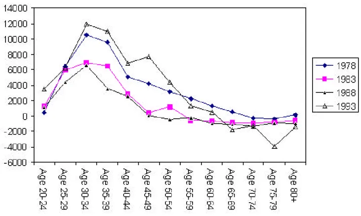
Figure A1(b) picks the 1993 mean profile and adds those from the other three waves,
1978-1983-1988. The shapes are roughly similar. Changes across years are far from a simple shift of each profile: for the younger age groups, 1988 was the year with highest financial saving, while there is less of a clear picture for the older ones.
Note: All data in prices of 1993 and weighted. Age/Cohort-groups denoted by begin of 5-year interval.
Source : Own calculations on the basis of the EVS 1978-1993.
Real Saving
Real saving consists of:
Purchases of, minus sales of, real estate (incl. owner-occupied housing)
plus expenditures in upkeep and improvement of housing, minus 2% depreciation plus amortization of, minus take-up of, mortgages
plus purchases of, minus sales of, gold and other jewelry.
The EVS data do not permit a sensible measurement of changes in wealth that is invested in business partnerships. This does affect only some households in a large way but not the average, see our companion paper. More serious are biases due to the fact that we do not have the regional information necessary to impute capital gains from real estate and business partnerships. Our measure of real saving is therefore less than satisfactory.
Figure A2 shows real saving, 1978-1993. It is dominated by saving and dissaving in
owner-occupied housing. The median is mostly zero and not shown, while the mean exhibits a very strong hump shape across age/cohort-groups with substantial dissaving for the older age groups.
Figure A2: Real Saving, 1978-1993
Note: All data in prices of 1993 and weighted. Source : Own calculations on the basis of the EVS 1978-1993.
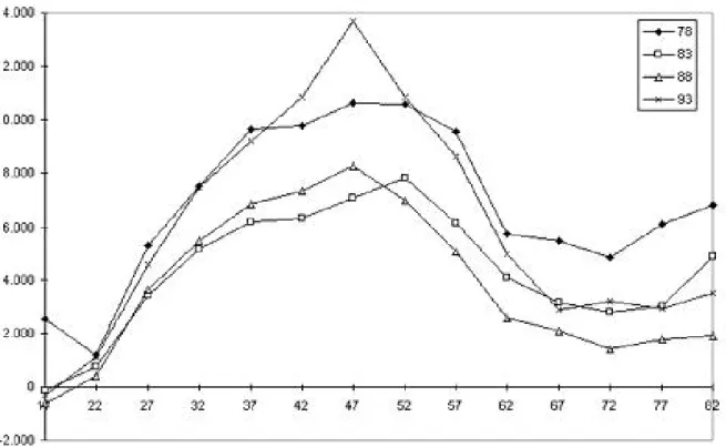
Figures A3(a) and (b) depict the sum of discretionary financial and real saving. Financial Saving dominates real saving in the flows, so total saving is positive for all but the very poor. Median and mean saving have the familiar hump shape, and remain positive for all age groups, except for the lower quartile.
Figure A3(a): Financial Saving in 1993
Figure A3(b): Mean Total Saving in 1978-1993
Note: All data in prices of 1993 and weighted. Age/Cohort-groups denoted by begin of 5-year interval.
Financial Wealth
The stocks of financial, real and total discretionary wealth are defined in accordance with the flow measures A1 through A3.
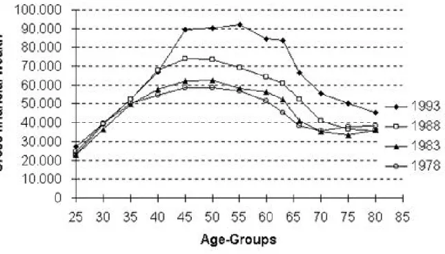
Age and cohort profiles of a longitudinal comparison of gross financial wealth for 1978 to 1993 are presented in Figure A4. Average real financial wealth has increased between 1978 and 1993 by 38 percent. This increase was mainly caused by a wealth expansion of middle age classes. The expansion of financial wealth is striking between 1988 and 1993. The reason is a large increase in securities ownership for all age classes. The development of gross financial wealth does not take into account an increase in loans, e.g. for the purchase of an apartment or house.
The composition of gross and net financial wealth in the four EVS waves is presented and discussed in Table II-2. There have been dramatic shifts: Traditional investment instruments like savings deposits or deposits with savings and loan associations have decreased by around 30 percent in real terms, while investments in securities have increased threefold. As a result the relative proportion of savings deposits and deposits with savings and loan associations has decreased from 47 to 25 percent. The proportion of life insurances was relatively stable.
Figure A4: Gross Financial Wealth, EVS 1978-1993 (Means)
Note: All data in prices of 1993. Age/Cohort-groups denoted by begin of 5-year interval.
Source : Own calculations on the basis of the EVS 1978-1993.
Real Wealth
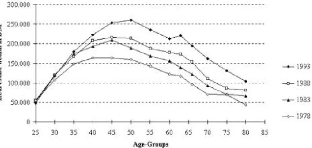
Average wealth in real estate property is presented in Figure A5 by age/cohort-class. We do not have a measure of business wealth in the EVS data.
Similar to financial wealth, wealth in real estate had increased until 1993. A more detailed analysis (Schnabel, 1998) shows that this is partly caused by the noticeable higher ownership rates in the EVS 1993. It is apparent from the EVS that ownership rates increased from cohort to cohort. Using the longitudinal SOEP data, one learns that ownership rates remain essentially constant with increasing age after age 60 for a given cohort.
Figure A5: Real Estate Wealth, EVS 1978-1993 (Means)
Note: All data in prices of 1993 and weighted. Age/Cohort-groups denoted by begin of 5-year interval.
Source: Own calculations on the basis of the EVS 1978-1993. Total Discretionary Wealth
Adding gross financial wealth (Figure A4), real estate wealth (Figure A5), and other real wealth and subtracting outstanding loans, we arrive at total discretionary wealth, as measurable in the EVS data. This measure omits business wealth, as noted before. Its age/cohort pattern is depicted in Figure A6.
West German private households possessed an average total wealth of DM 245,000 (
122,000). The largest part was real estate. For the group aged 30 to 59 this makes 80 to 90 percent of total wealth. The most important part of this is homeownership.
At the time of the head,s retirement an average German household owned around DM 275,000 ( 138,000) of total wealth in 1993. This is 12.5 times the public pension of an average
employee with 45 years of service in 1993 (net DM 22,000, 11,000). The median wealth is DM 200,000, ( 100,000) which is lower than the mean but still relatively high. Thus, it could quite substantially contribute to consumption - especially in old age (Schnabel, 1999).
Nevertheless, accumulation of even more wealth in the form of financial wealth takes place on average in old age, as was illustrated in the savings profiles presented earlier. This is a
Figure A6: Total Discretionary Wealth, EVS 1978-1993 (Means)
Note: All data in prices of 1993 and weighted. Age/Cohort-groups denoted by begin of 5-year interval.
Source : Own calculations on the basis of the EVS 1978-1993. Mandatory Saving
Germany has essentially no mandatory contributions to public funded pension plans. Only a minority of civil servants are required to contribute a small percentage of their salary increases to funds that are effectively invested in government bonds. The contributions amount to roughly 0,5% of salary.
Many companies offer private pension plans to their employees. In many cases, they are mandatory in the sense that they come as package deals with the employment contract with no opt-out possibilities. Contributions are shared between worker and company at various percentages ranging from all employer paid to equally shared. Actual economic incidence is of course another matter.
Although more than 50% of workers are covered by a firm pension at least part of their career, firm pensions play a small role in Germany. On average, about 5-6 percent of
retirement income comes from employer provided pensions although some companies have generous funded pension plans. Most of these plans invest in the own firm ("book reserves") although recently several companies started to offer pension plans that invest in the capital market at large.
Contributions to Pay-as-you-go Systems
All dependent employees and their employers must contribute to the German retirement insurance system which is unfunded. The contribution rate is currently (2000) 19.3% of gross earnings. In addition, an estimated 8.5% of gross earnings is levied indirectly via other taxes,
mainly V.A.T. and the new eco-tax, see Figure C1 below.
The contribution base for public pension contributions is capped at about 1.6 times the average earnings. High wage earners therefore pay a lower percentage of their income (and will receive a lower replacement rate in accordance, see Part II).
Coverage of workers is about 85 percent. The remaining workers are self-employed (who could contribute to the public pay-as-you-go scheme but do not do so, although this was different in the mid 1970s), civil servants (who receive pensions direct from the state budget and, at least implicitly, pay contributions through lower salaries than their private business
counterparts), and workers who earn less than a threshold that is currently about 15% of the average wage. Since 1999, the latter group pays a reduced contribution rate, mainly through the employer.
Social insurance also covers health, long-term care, and unemployment insurance. For most workers, again excluding the self-employed, civil servants, and low earners, they add up to another 21 percent of gross income, with a tax base capped similarly as the contributions to the public pension system.
Since contributions are proportional to earnings up to the earnings ceiling, they essentially follow the life-cycle pattern of income which we turn to in the following section.
Figure C1: Contribution rates to public pension system
Total Gross Income
In order to compute saving rates and a residual saving measure, we need an income base which is defined internally consistent with our saving and wealth concepts. Total gross income is:
plus asset income from financial and real assets
plus annuitized pensions from the public PAYG pension system plus annuitized and lump-sum company pensions
plus net family transfers, including alimonies received minus those paid, and regular as well as one-time inter vivos transfers.
plus all other public transfers except public pensions (mainly social assistance, unemployment compensation, and family allowances)
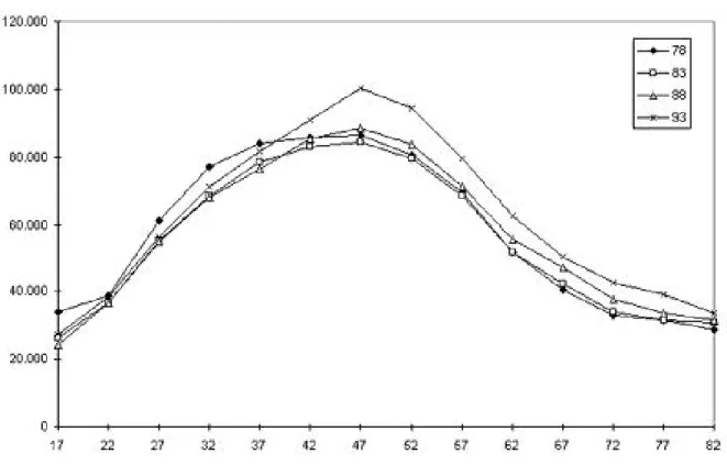
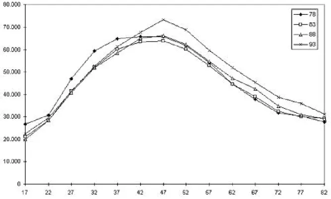
Figure D1 depicts total gross income for all four waves. We see the familiar hump shape pattern but should be warned again: the actual life-cycle pattern is much flatter as each later cohort profits from the secular productivity increase, shifting the cross-sectional lines to the right from wave to wave, see Section Ib.
Figure D1: Total gross income
Note : All data in prices of 1993. Age/Cohort-groups denoted by midpoint of 5-year interval.
Source : Own calculations on the basis of the EVS 1978-1993. Total Disposable Income
Disposable income is simply gross income minus direct taxes (Federal income tax) minus the contributions to mandatory social security systems that were mentioned in section C. Disposable income is about DM 50.000 ( 25,000) p.a. for the average household in the sample. It is 30 percent higher at the peak ages from 40 to 50 years, and about 30 percent lower for the older age groups and cohorts, see Figure D2. Compared to gross income, disposable income is roughly two thirds of this. The median is 10-20 percent lower than the
mean, see Table D2 in the appendix, pointing to a considerably less skewed income distribution than, e.g., in the United States.
Figure D2: Total Disposable Income
Note : All data in prices of 1993. Age/Cohort-groups denoted by midpoint of 5-year interval.
Source : Own calculations on the basis of the EVS 1978-1993.
Annuitized Retirement Income
Annuitized income dominates retirement income in Germany. It consists of private and
(mostly) public pensions. Less frequent are annuities from life insurance contracts, although this will change in the future when the current working generation will retire.
Table D3 in the appendix details annuitized retirement income. For the young households, this income mainly includes survivor pensions that are paid to widows and (half-)orphans.
Saving as Residual
The tables in Section A were based on flows, such as purchases and sales of assets during one calendar year. In this section, we compute saving as a residual, subtracting all consumption expenditures from disposable income (Section D). Consumption expenditures are reported fairly detailed in the EVS, based on weekly diaries. Expenditure categories are enumerated in Börsch-Supan et al. (1999).
Note: All data in prices of 1993. Age/Cohort-groups denoted by midpoint of 5-year interval.
Source : Own calculations on the basis of the EVS 1978-1993.
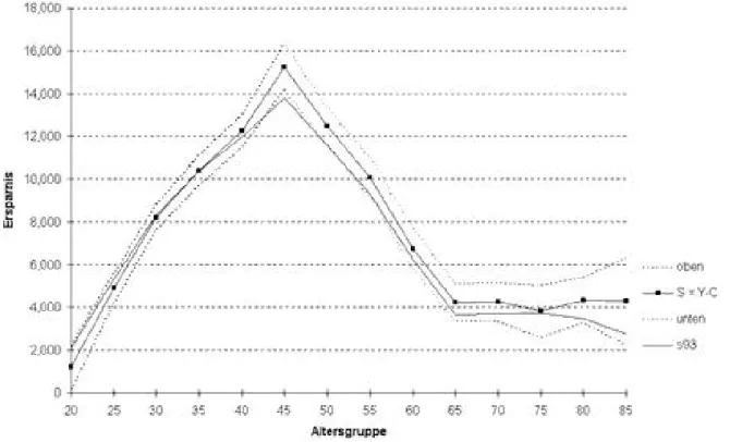
The discrepancy between the two savings measures is very small. As Figure E2 shows, the flow measure of saving is almost always within the 2 -confidence bands of the residual measure. Using confidence bands for both measures, the difference is not significant. This is an important result as it strengthens the belief in the internal consistency of the data. Nevertheless, our companion paper details that there are important departures from coincidence for some households which are masked by the averages depicted in Figure E2.
Note: All data in prices of 1993. Age/Cohort-groups denoted by begin of 5-year interval.
Source : Own calculations on the basis of the EVS 1978-1993.
Saving Rates
We finally compute saving rates. Because mean saving rates are very sensitive to changes in nominator and denominator, we focus on the median and quartile saving rates in each age category, see Figure F1 below. This figures shows that the age/cohort pattern is rather stable across income quartiles. The differences (pronounced hump shape for the richer, fairly flat for the poorer households) are thus mainly due to differences in income profiles. The increase in saving rates in very old age is interesting. Remember, however, that the data only covers households, not elderly in institutions. Thus, the sample selects those who are less likely to dissave. A back-on-the-envelope calculation (Börsch-Supan, 1992) shows that this selection effect by itself cannot explain the high saving rates in old age, but without
longitudinal data, no final analysis is possible.
Note: All data in prices of 1993. Age/Cohort-groups denoted by begin of 5-year interval.
Source : Own calculations on the basis of the EVS 1978-1993.
The different measures of saving (A=flow, E=residual) in Figures F2(a) and (b) appear to exhibit rather different qualitative patterns. Measure E shows even less of a typical life-cycle pattern than one might expect. In addition to the now frequently reiterated caveat, that these profile present a mixture of cohort and age effects and do not identify life-cycle changes, one also needs to take the large standard deviations into account: The saving rates depicted by Figures F2(a) and (b) are only weakly different in a statistical sense for the old-age groups. Thus, the proximity between the absolute saving measures in Figures E2 (a) and (b) is no contradiction to the apparent difference in Figures F2 (a) and (b). Particular at the low income end, saving rates are typically a division of small amounts of saving that exhibit high variation by small incomes that equally variable.
Figure F2(b): Saving Rates, 1978-93 (Based on Residual Saving Measure E)
Note: All data in prices of 1993. Age/Cohort-groups denoted by begin (Fig.F2a) and
midpoint (Fig. F2b) of 5-year interval.
Covariates
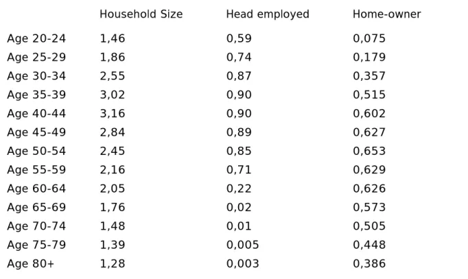
The table below shows that "households" are not a stable concept over time in order to analyze saving behavior. Household size changes from 1.5 at age 20-24 to about 3.2 at age 40-44, then returns to the initial value at age 70 and declines even further. This is an
important insight as it implies that life-cycle models of saving behavior have to jointly model the change in household composition, at least the change in household size.
Employment status has the typical pattern for mid-European countries: virtually everybody is retired at age 65. Homeownership depicts a mixture of age and cohort effects. Since it is well-known from longitudinal data (e.g., GSOEP) that few elderly move in old age, the apparent decline of homeownership in old age is purely a cohort effect.
Table G: Household Characteristics
Household Size Head employed Home-owner
Age 20-24 1,46 0,59 0,075 Age 25-29 1,86 0,74 0,179 Age 30-34 2,55 0,87 0,357 Age 35-39 3,02 0,90 0,515 Age 40-44 3,16 0,90 0,602 Age 45-49 2,84 0,89 0,627 Age 50-54 2,45 0,85 0,653 Age 55-59 2,16 0,71 0,629 Age 60-64 2,05 0,22 0,626 Age 65-69 1,76 0,02 0,573 Age 70-74 1,48 0,01 0,505 Age 75-79 1,39 0,005 0,448 Age 80+ 1,28 0,003 0,386
Source : Own calculations on the basis of the EVS 1993.
Note that virtually all households in Germany have health insurance. It is mandatory except for the upper 15% of the income distribution, and almost all of the latter households have private health insurance. Germany also has a mandatory long-term care insurance.
Cohort Profiles
As already stressed at several times in this paper, the tables in Part Ia display cross-sectional variation across age/cohort-groups and do not identify life-cycle changes. In order to do
understand life-cycle behavior, we need to follow households over time. In lack of longitudinal data on savings in Germany, we combine the data of the available four EVS cross-sections from 1978 to 1993 and construct a synthetic panel of groups of households by identifying households in subsequent five-year age-groups with each other, i.e., by identifying the 45-49
year old persons in 1978 with the 50-54 year old persons in 1983, the 55-59 year old persons in 1988, and the 60-64 year old persons in 1993.
We then construct cohort-specific age savings profiles under the identifying assumption that time effects are zero. Under this assumption, discussed at length in Chapter X of this volume, "pure" age effects are visible when points of neighboring age groups are connected as they proceed in time, i.e., by connecting the age groups as described at the end of the preceding paragraph. The three examples in Figure 1, derived from, and to be compared with, Figure A6 in Part Ia, make the point:
Figure Ib-1: Total Discretionary Wealth by Cohort
Notes and Sources: See Figure A6.
Figure 2 displays total discretionary saving by cohort, starting at the left side with the youngest cohort in our data, born between 1954 and 1958, and proceeding to the oldest cohort, born between 1909 and 1913.
Saving increases until it reaches a peak in the age range 45-49, then declines until the age group of the 65-69 old. It then remains essentially flat. As already stated several times, saving remains positive even in old age, according to these data.
Note: All data in prices of 1993. Age-groups denoted by begin of 5-year interval.
Source: Schnabel (1999)
The life-cycle pattern in saving visible in Figure 2 has two components, displayed in Figures 3 and 4. First, savings rates exhibit much less of a hump-shaped pattern than total saving. The are fairly stable around 12% for all young and middle-aged groups until around age 45-49. They then decline and stabilize around age 65-69, when they remain at about 4%. The data suggests an increase for the 1988 wave for all older cohorts. We have no satisfactory explanation for this effect, particularly, because the pension level decreased between 1983 and 1988.
Note: All data in prices of 1993. Age-groups denoted by begin of 5-year interval.
Source: Schnabel (1999)
Figure Ib-4: Disposable Income by Cohort (Means)
Note: All data in prices of 1993. Age-groups denoted by begin of 5-year interval.
Figure 4 shows the second component of the life-cycle changes in total discretionary saving, namely the change in disposable household income. Income rises until about the 45-49 age group, then declines when household sizes become smaller (see Section G in Part Ia) and transfer income frequently changes sign (from receiving family allowances to giving inter family transfers). From age-groups 55-59 onwards, we also see the effects of declining labor force participation, i.e., pre- and early retirement.
The positive saving rates throughout all age-groups are reflected in the life-cycle pattern of wealth, see Figure 5 below. Total discretionary wealth increases until late in life.
Figure Ib-5: Total Discretionary Wealth by Cohort (Means)
Note: All data in prices of 1993. Age-groups denoted by begin of 5-year interval.
Source: Schnabel (1999)
Policies Affecting Saving
Our main finding is an age-saving profile which exhibits only a mild hump-shape. The profile is much flatter than, e.g., in the US. Savings remain positive in old age, even for most low income households. The overall saving rate is high relative to many other countries.
How can we explain this pattern? This is the aim of the second part of this paper. It attempts to link the observed savings pattern with public policies affecting saving behavior. Public policies include capital taxation and subsidies to specific forms of saving and, most notably, the public pension system.
To this end, we first very briefly describe the German public social insurance system as it relates to savings. We find that Germany has a very generous public pension and health
insurance system, particularly considering the early retirement and disability options that permit retirement around age 60 with little or no reduction in pension income. Thus, we have a "German savings puzzle": Pensions and health insurance are generous and likely to have large crowding out effects, yet private savings are high until old age.
We need a complicated answer to explain this puzzle. It combines historical facts with capital market imperfections and a distinction between the role of discretionary and mandatory savings.
The last section of this part of the paper deals with other savings incentives, mainly the German system of capital taxation and dedicated savings incentives which have shaped the portfolio composition of German savings.
The German Pension System
Germany has a contribution-based PAYG system. It is very monolithical, covering almost all workers and providing almost all retirement income in a single system with relatively
transparent rules. Until recently, it has been successful in providing a high and reliable level of retirement income and was praised as one of the causes for social and political stability in Germany. It has survived two major wars, the Great Depression, and more recently,
unification. However, times have changed, and a flurry of reforms since 1992 has not
succeeded in stabilising contribution rates, public support, and system enrolment. There are two main reasons for the increasing difficulties of the German public pension system:
population ageing and negative incentive effects on labour supply.
As opposed to other countries such as the United Kingdom and the Netherlands, which originally adopted a Beveridgian social security system that provided only a base pension, public pensions in Germany were from the start designed to extend the standard of living that was achieved during work life also to the time after retirement. Thus, public pensions are roughly proportional to labor income averaged over the entire life course and feature only few redistributive properties. Benefits include old-age pensions, survivor benefits at 60% of
old-age pensions, and disability benefits exceeding old-age pension benefits before age 65. Benefits are computed on a life-time contribution basis. They are the product of four elements: (1) the employee,s relative wage position, averaged over the entire earnings history, multiplied by (2) the number of years of service life and (3) adjustment factors for pension type (old-age and two disability pension types) and retirement age (since the 1992 reform), both in turn multiplied by (4) the average pension level that is indexed "dynamically" (i.e., during the entire retirement period) to the current average net wage of the working population. Until 1992, indexation was to gross wages. The first three factors make up the "personal pension base" while the fourth factor determines the income distribution between workers and pensioners in general. The wage indexation has kept the income distribution between workers and pensioners constant as it has automatically transferred productivity gains also to pensioners. We will come back to the effect of this indexation scheme in the next subsection.
The German retirement insurance system has a high replacement rate, generating net
retirement incomes that are currently about 70 percent of pre-retirement net earnings for a worker with a 45-year earnings history and average life-time earnings. The corresponding net replacement rate in the US is about 53 percent. The German retirement insurance system
also provides generous survivor benefits that constitute a substantial proportion of the expected pension wealth of married couples, and disability benefits at similar and sometimes even higher replacement levels than old-age pensions.
Early retirement provisions substantially contribute to the generosity. The 1972 pension reform introduced the opportunity to retire at different ages ("flexible retirement") during a "window of retirement." This window began at age 60 for women, unemployed, and workers who could not appropriately be employed for health or labour market reasons. It began at age 63 for workers with a long service history (35 years, including higher education, military service, a certain number of years for rising children, etc.). Normal retirement age was (and still is) age 65. The 1972 reform did not introduce an actuarial adjustment. The reforms in the 1990s will shift the window of retirement for all workers to age 62 and will include an adjustment of benefits. However, this adjustment will be about half of the actuarially fair adjustment. The introduction of early retirement in 1972 had a huge impact on retirement age
(Börsch-Supan and Schnabel, 1998). Within a few years, retirement age among men dropped by about 3 years and average retirement age fell below age 60. The resulting distribution of retirement ages became marked by distinct "spikes" at ages 60, 63 and 65. The retirement age of 65 now mostly applies to women with a very short earnings history, while the most popular retirement age among men became age 60. Since average life expectancy of a male worker at age 60 is about 18 years, the earlier retirement age amounts to an increase in pension expenditures of about 15 percent. The effect is smaller, but still significant, for women.
Disability status is granted for medical reasons. In this case, no actuarial adjustments apply, even after the 1992 reform. Moreover, pensions received before age 60 are calculated as if the worker had worked to age 60. Incentives to take up disability pensions are thus strong if one manages to claim full disability status. Disability status is also given for economic
reasons, for instance, when a worker could not find a job at all, or could not find an appropriate job. In the latter case, a lower replacement rate applies.
The German public pension system provides two floors for retirement income. First,
contributions below a certain minimum have ex post been topped up to lie between 50 and 75 percent of average contributions. Although not an entitlement by the law, the Bundestag has regularly enacted such ex post adjustments to poor workers earnings histories, and has thereby effectively introduced a minimum pension. Second, social assistance provides a
minimum income to which all Germans are entitled. Older households receive a higher minimum income than younger households (about 600 for single elderly, 900 for an elderly couple, including housing assistance).
The topping up mechanism has generated a redistributive element along the income scale into the German retirement "insurance". However, social assistance is quantitatively more
important, and has effectively shielded the elderly from poverty. Poverty rates among the elderly are much lower in Germany than in the United States and in the United Kingdom (Börsch-Supan, Reil-Held and Schnabel, 1999).
The German Health Insurance System
Similar to the pension system, the German health insurance is generous and has effectively shielded all households from illness-related poverty. It is contribution-based, and enrolls about
85% of all German persons. The self-employed and those with earnings above a threshold of about 135% of average wages can opt out. For all others, the system is mandatory. Civil servants have their own system. Workers remain enrolled when they retire. The public health insurance system must enroll everyone who applies, but once opted out, there is no way back in.
The public health insurance covers ambulatory and hospital services, medication and supplies. There is no coinsurance, although a (relatively low) fixed fee is charged for each doctoral visit, hospital stay and prescription. Recently, a list has banned certain medications (e.g., against the common cold) and tighter restrictions have been put on spa visits. Nevertheless, health insurance is still essentially universal.
The health insurance is complemented by a long-term care insurance which covers between a third and a half of nursing home and in-house care. Like health insurance, it is a contributory PAYG system.
The German Unemployment Insurance System
The third branch of the German social insurance scheme is unemployment insurance, providing unemployment compensation and unemployment aid. In a nutshell, unemployment compensation provides during one year a replacement rate between 63% and 68% of last earnings, depending on the number of children. Unemployment aid follows, with a replacement rate between 56 and 58%, with no duration limitation.
We claim that the generosity and specific incentive effects of the German social insurance system have significantly influenced savings behavior in Germany. We distinguish three distinct types of effects: effects on the level of savings, essentially by crowding-out
mechanisms; effects on the life-cycle pattern of savings, flattening the age-savings profile; and effects on the portfolio composition of savings.
Crowding-Out Effects
The generosity of the German pension system and the broad insurance it gives also to survivors and disabled workers is likely to crowd out private old-age provision. Indeed, the German composition of retirement income is much more dominated by public pensions than in the other countries in Table II-1 below:
Table II-1: Retirement Income by Pillar (percentages)
Germany The Netherlands Switzerland UK US
State 85% 50% 42% 65% 45%
Employer 5% 40% 32% 25% 13%
Individual 10% 10% 26% 10% 42%
Notes: Income composition of two-person households with at least one retired person. UK: "State" includes SERPS. US: "Individual" includes earnings (25%).
This table shows that Germany holds an extreme position with a very thick public PAYG pillar and very thin private pillars. About 85% of retirement income stems from the public
mandatory retirement insurance, and only 15% come from private sources such as funded firm pensions and individual retirement accounts, labour income, and family transfers.
The substitution result is in line with a time-series analysis of Kim (1992). He links changes in the retirement system to the savings rate and shows that the German pay-as-you-go system has crowded out saving to a significant extent. While there are many confounding factors in either analysis, and while no single econometric analysis can be the ultimate conclusive evidence, Kim,s analysis is careful and econometrically convincing.
However, Table II-1 is at odds with the fact, that Germany has such a high saving rate.
Moreover, we saw in Part I of this paper that in particular the German elderly had astonishing high saving rates and financial wealth levels that suffice for about 10 years of retirement income (see Section A6 in Part Ia). This is the core of the "German savings puzzle". We need two elements to explain it.
Schnabel (1999) provides the first element of our explanation. He shows that the growth of income during the German economic miracle years and up to the seventies was so large and unprecedented that the elderly could just not have anticipated it. Figure II-1 displays the growth of earnings during the work history of a typical worker who retired in 1970, the jump due to the 70% replacement rate after retirement, and then the subsequent increase in pension income due to gross indexation. All numbers are in real terms. After less than 10 years, the average workers had essentially recouped their former earnings. The process was only stopped in the early eighties, when economic growth substantially slowed down in
Germany.
Source: Schnabel (1999)
Since this income path could hardly be anticipated, workers consumed "too little", and ended up with too large a stock of wealth around retirement.
The second element of our explanation of the German savings puzzle needs to explain why this wealth has not been spent at higher rates in old age. This is a difficult task. One explanation is habit formation: the elderly did not want to change the accustomed level of consumption which they have learned some 50 years ago. We are aware that economists do not like this kind of explanation but there appears some truth to it. Börsch-Supan and Stahl (1991) provide a complementary explanation. They argue that due to deteriorating health conditions, the elderly are simply less able to spend as much as they would need to make saving negative. Note also, that annuitized pension income cannot be borrowed against even if the elderly had anticipated the decline in health and their inability to draw down wealth at later ages.
Life-Cycle Saving Patterns
This two-element explanation is consistent with the relatively flat life-cycle savings profiles in Germany. We refer to Figure A1 in the Part Ia of the paper and its longitudinal equivalents in Part Ib.
It is helpful to distinguish the older generation, born before 1930 and retired before 1995 (depicted in Figure II-1) from the younger generation born after World War II, not yet retired. The older generation experienced during their working lives a spectacular and unexpected income growth. The younger generations, experience was that of a constant comfortable level of economic fortune in Germany.
We explained the older generations, savings habits in the preceding subsection: They may have had a retirement savings motive, but they were surprised by their high retirement income and could not draw down. A relatively flat savings profile emerged.
The younger generation in Germany learned that retirement is not a time of scarce resources. For them, the high replacement rates of the German public pension system made additional private retirement provision largely unnecessary. Thus, saving for retirement, the only motive under the pure life-cycle hypothesis, was of secondary importance. Other saving motives dominated, such as high frequency precautionary saving, high frequency saving for durables such as cars, and saving for intergenerational transfers. Again, this implies that age-saving profiles are much flatter than under the retirement-saving oriented life-cycle hypothesis. Indeed, inter vivos transfers are high and survey questions on savings motives show an almost equal spread between the four mentioned saving motives.
We are aware that our explanation may be suggestive and plausible, but that the line of argument is vulnerable because we lack a counterfactual. We hope that international
comparisons will help to overcome this problem. In fact, the hump-shaped life-cycle savings pattern is most pronounced in the U.S. where the replacement rates of the public PAYG
pension systems are lower - and thus the retirement savings motive is more important - than in continental Europe.
the (in part unexpectedly) generous retirement benefits from the PAYG pension system due to the rapid growth of the economy in the post-war period, we should expect changes in saving patterns in the future. Growth rates have declined and the dependency ratio is deteriorating rapidly. This implies that the current generosity of the PAYG system is unlikely to prevail. This will revive the retirement motive for saving. Hence, saving rates among the young will increase to accumulate retirement savings, and saving rates among the elderly will decline sharply because they will dissolve their retirement savings. We might have to wait for this
counterfactual to obtain a clearer explanation of what caused the puzzling German savings behavior.
Portfolio Composition
The German PAYG public pension system appears also to have shaped the composition of household wealth. As pointed out in Section A6, the largest part was real estate. For the group aged 30 to 59 this makes 80 to 90 percent of total wealth. At the time of the head,s retirement an average German household owned around DM 275,000 ( 138,000) of total wealth in 1993. This is about the same as the present discounted value of public pensions at that time. Average net financial wealth, on the other hand, is only DM 28,000 ( 14,000). Of course, this only reflects what we have seen in Table II-1.
Table II-2 displays the portfolio choice of this relatively small residual financial wealth in the 1993 wave of the EVS.
Table II-2: Composition of household wealth, Germany, 1978-1993
1978 1983 1988 1993 Share in 1993
Savings accounts 15.534 12.224 13.287 11.120 17.5%
Building societies 6.225 5.957 4.998 4.744 7.5%
Stocks and bonds 7.430 8.957 10.381 19.948 31.4%
Life insurance (cash value) 16.719 16.821 22.379 21.141 33.3%
Other financial wealth - 1.811 1.784 6.614 10.4%
Gross financial wealth 45.909 45.770 52.830 63.567 100.0% ./. consumer loans 23.043 28,859 30.266 35.055
Net financial wealth 22.866 16.912 22.563 28.512
Note: Household data from the Einkommens- and Verbrauchsstichprobe (EVS). All figures in DM and in 1993 prices.
Source: Börsch-Supan et al. (1999).
The most important component is whole life insurance, about a third of gross financial wealth. The central reason for the important role of whole life insurance in German households
life-cycle savings decisions is its favorable tax treatment (see Brunsbach and Lang, 1998, and Walliser and Winter, 1999). At the household level, saving in whole life insurance is more
important than saving in stocks and bonds. Bonds make up the lions, share in this category, while stocks are less than 10 percent of the average household portfolio. This fact is also significant for financial markets, as life-insurance companies are not allowed to invest significantly in stocks, which in turn is one of the main reasons for thin capital markets in Germany (see Deutsche Bank Research, 1996).
It is highly speculative how this portfolio composition would change under a partial transition to prefunding. If there were no substitution between new retirement saving and current saving, the household saving rate would increase by between 2 and 4 percent, see Birg and
Börsch-Supan (1999). If all of this would be channeled into pension funds, which only recently have been introduced in Germany and still do not receive preferential tax treatment similar to whole life insurance, pension funds would amount to between 15 and 18 percent of households, portfolios, comparable to the United Kingdom, the U.S., the Netherlands and Switzerland.
Substitution between new retirement saving and current saving would increase this share, but part of new retirement saving may also be done as whole life insurance. Households, direct and indirect exposure to stock markets then depends on future investment decisions of life
insurance companies who only recently began to increase their portfolio share of stocks. Judging from the international experience in countries as diverse as the United Kingdom, the U.S., the Netherlands and Switzerland, a more prominent role of equities on the supply side of the capital markets seems very likely when more of the German retirement income will be prefunded.
Tax Policies Affecting Saving
Section still under construction.
(a) Brief description of tax treatment of capital income, homeownership, whole life insurance, pension funds
(b) Results. The main messages are:
no capital gains taxation, but capital income taxed at high rate. Favors stocks over bonds.
homeownership discouraged for median income since tax benefits for landlord higher than for median income renter.
Tax subsidies for dedicated savings (whole life insurance, Bausparkassen) have been large, they are now rather small. The decline of Bausparkassen savings is visible in Table II-2. No decline for whole life insurances, probably because of compensating effect through incerase in private old-age provision, see earlier part of section. Tax incentive effects on dedicated savings probably negligible at this point.
No level playing field for pension funds: no tax advantage at all. References
Becker, I. (1997): Die Entwicklung von Einkommensverteilung und Einkommensarmut in den alten Bundesländern von 1962 bis 1988. In: I. Becker und R. Hauser (Hg.):
Einkommensverteilung und Armut. Deutschland auf dem Weg zur Vierfünftel-Gesellschaft?
Campus Verlag, Frankfurt New York.
Börsch-Supan, A. (1992): Saving and consumption patterns of the elderly: the German case.
Journal of Population Economics , 5, 289-303.
Börsch-Supan, A. (1999): Zur deutschen Diskussion eines Übergangs vom Umlage- zum Kapitaldeckungsverfahren in der Gesetzlichen Rentenversicherung. Finanzarchiv , im Erscheinen.
Börsch-Supan, A. and A. Reil-Held (1998): Retirement income: level, risk, and substitution among income components. OECD Ageing Working Paper AWP 3.7 . Paris.
Börsch-Supan, A., A. Reil-Held and R. Schnabel (1999): Pension provision in Germany. In: P. Johnson (Hg.): Pensioners, Income: International Comparisons . Cambridge, MA and London: MIT-Press. Im Erscheinen.
Börsch-Supan, A., A. Reil-Held, R. Rodepeter, J. Winter and R. Schnabel (1999):
Ersparnisbildung in Deutschland: Meßkonzepte und Ergebnisse auf Basis der EVS, Arbeitspapier Nr. 99-02, Sonderforschungsbereich 504, Universität Mannheim.
Börsch-Supan, A., R. Rodepeter and J. Winter (1999): The empirical identification of life-cycle savings patterns. Unveröffentlichtes Manuskript, Universität Mannheim.
Börsch-Supan, A. and K. Stahl (1991): Life-cycle savings and consumption constraints.
Journal of Population Economics , 4, 233-255.
Browning, M. and A. Lusardi (1996): Household saving: macro theories and micro facts.
Journal of Economic Literature , 34, 1797-1855.
Deaton, A. (1985): Panel data from time-series of cross-sections. Journal of Econometrics , 30, 109-124.
Disney, R., M. Mira d,Ercole and P. Scherer (1998): Resources during retirement. OECD Ageing Working Paper AWP 4.3 . Paris.
Euler, M. (1985): Geldvermögen privater Haushalte Ende 1983. Wirtschaft und Statistik , Heft 5, 408-418.
Euler, M. (1990): Geldvermögen und Schulden privater Haushalte Ende 1988, Wirtschaft und Statistik , Heft 11, 798-808.
Euler, M. (1992): Einkommens- und Verbrauchsstichprobe 1993. Wirtschaft und Statistik , Heft 7, 463-469.
Fachinger, U. (1998): Die Verteilung der Vermögen privater Haushalte: Einige konzeptionelle Anmerkungen sowie empirische Befunde für die Bundesrepublik Deutschland. ZeS-Arbeitspapier Nr. 13/98, Zentrum für Sozialpolitik, Universität Bremen.
Fitzenberger, B., R. Hujer, T.E. MaCurdy and R. Schnabel (1998): Testing for uniform wage trends in West Germany: A cohort analysis using quantile regression for censored data. Unveröffentlichtes Manuskript, Universität Mannheim.
Guiso, L., T. Jappelli and D. Terlizzese (1994): Why is Italy,s saving rate so high? In: A. Ando, L. Guiso and I. Visco (Hg.): Saving and the Accumulation of Wealth. Essays on Italian Household and Government Saving Behaviour . Cambridge, MA: Cambridge University Press.
Guttmann, E. (1995): Geldvermögen und Schulden privater Haushalte Ende 1993. Wirtschaft und Statistik , Heft 5, 391-399.
Hauser, R. (1997): Armut, Armutsgefährdung und Armutsbekämpfung in der Bundesrepublik Deutschland. Jahrbücher für Nationalökonomie und Statistik , Bd. 216, 524-548.
Hauser, R. and I. Becker (1998): Die langfristige Entwicklung der personellen
Einkommensverteilung in der Bundesrepublik Deutschland. In: H.P. Galler und G. Wagner (Hg.):
Empirische Forschung und wirtschaftspolitische Beratung . Campus Verlag, Frankfurt/New York.
Hauser, R. and U. Neumann (1992): Armut in der Bundesrepublik Deutschland. Die
sozialwissenschaftliche Thematisierung nach dem Zweiten Weltkrieg. In: Armut in modernen Wohlfahrtsstaaten . Sonderheft 32/1992 der Kölner Zeitschrift für Soziologie und
Sozialpsychologie.
Helmcke, T. and P. Knoche (1992): Zur faktischen Anonymität von Mikrodaten. Wirtschaft und Statistik , Heft 3, 139-144.
Hertel, J. (1997): Einnahmen und Ausgaben der privaten Haushalte 1993. Statistische Bundesamt, Fachserie 15, Heft 4, 28-41.
Kim, S., (1992): Gesetzliche Rentenversicherung und Ersparnisbildung der privaten Haushalte in der Bundesrepublik Deutschland von 1962 bis 1988, Zeitschrift für die gesamte
Versicherungswirtschaft 81 , 555-.
Lang, O. (1996): Die Einkommens- und Vermögensverhältnisse künftiger Altengenerationen in Deutschland. In: Deutscher Bundestag (Hg.): Herausforderungen unserer älter werdenden Gesellschaft an den einzelnen und die Politik . Studienprogramm der Enquete-Kommission "Demographischer Wandel".
Lang, O. (1997): Steueranreize und Geldanlagen im Lebenszyklus. Dissertation, Universität Mannheim.
Laue, E. (1995): Grundvermögen privater Haushalte Ende 1993. Wirtschaft und Statistik , Heft 6, 488-497.
Modigliani, F. and R. Brumberg (1954): Utility analysis and the consumption function: an interpretation of cross-section data. In: J.H. Flavell and L. Ross (Hg.): Social Cognitive Development Frontiers and Possible Futures . Cambridge, NY: University Press.
Münnich, M. (1997): Zur wirtschaftlichen Lage von Ein- und Zweipersonenrentnerhaushalten.
Wirtschaft und Statistik , Heft 2, 120-135.
Pöschl, H. (1993): Werbung und Beteiligung der Haushalte an der Einkommens- und Verbrauchsstichprobe 1993. Wirtschaft und Statistik , Heft 6, 385-390.
Poterba, J. M. (Hg.) (1994): International Comparisons of Household Saving . Chicago, IL: University of Chicago Press.
Reil-Held, A. (1999): Bequests and aggregate wealth accumulation in Germany. The Geneva Papers on Risk and Insurance , 24, 50-63.
Rodepeter, R. and J. Winter (1998): Savings decisions under life-time and earnings uncertainty: evidence from West German household data. Arbeitspapier Nr. 98-58, Sonderforschungsbereich 504, Universität Mannheim.
Schnabel, R. (1999): Ersparnis und Vermögen im Lebenszyklus in Westdeutschland . Habilitation, Universität Mannheim.
Statistisches Bundesamt (1998): Erste Ergebnisse aus der Einkommens- und Verbrauchsstichprobe 1998. Mitteilungen für die Presse 362/98.
Walliser, J. and J. Winter (1998): Tax incentives, bequest motives and the demand for life insurance: evidence from Germany. Unveröffentlichtes Manuskript, Universität Mannheim.