Automated Generation of Computationally Hard Feature Models using
Evolutionary Algorithms
Sergio Seguraa,∗, Jos´e A. Parejoa,∗∗, Robert M. Hieronsb, David Benavidesa, Antonio Ruiz-Cort´esa
aDepartment of Computer Languages and Systems, University of Seville Av Reina Mercedes S/N, 41012 Seville, Spain
bSchool of Information Systems, Computing and Mathematics, Brunel University Uxbridge, Middlesex, UB7 7NU United Kingdom
Abstract
A feature model is a compact representation of the products of a software product line. The automated extraction of information from feature models is a thriving topic involving numerous analysis operations, techniques and tools. Per-formance evaluation in this domain typically relies on the use of randomly generated feature models. However, these only provide a rough idea of the behaviour of the tools with average problems and do not reveal their real strengths and weaknesses. In this article, we propose to model the problem of finding computationally hard feature models as an optimisation problem and we solve it using a novel evolutionary algorithm for optimised feature models (ETHOM). Given a tool and an analysis operation, ETHOM generates input models of a predefined size maximising aspects such as the execution time or the memory consumption of the tool when performing the operation over the model. This allows users and developers to know the performance of tools in pessimistic cases providing a better idea of their real power and revealing performance bugs. Experiments using ETHOM successfully identified models producing much longer executions times and higher memory consumption than those obtained with randomly generated models of identical or even larger size.
Keywords: Search-based testing, software product lines, evolutionary algorithms, feature models, performance testing, automated analysis.
1. Introduction
1
Software Product Line (SPL) engineering is a
sys-2
tematic reuse strategy for developing families of
re-3
lated software systems [16]. The emphasis is on
de-4
riving products from a common set of reusable assets
5
and, in doing so, reducing production costs and time–
6
to–market. The products of an SPL are defined in terms
7
of features where a featureis any increment in
prod-8
uct functionality [6]. An SPL captures the
commonal-9
ities (i.e. common features) and variabilities (i.e.
vari-10
ant features) of the systems that belong to the product
11
line. This is commonly done by using a so-called
fea-12
ture model. Afeature model[32] represents the
prod-13
ucts of an SPL in terms of features and relationships
14
amongst them (see the example in Fig. 1).
15
∗
Principal corresponding author
∗∗
Corresponding author
Email addresses:[email protected](Sergio Segura),
[email protected](Jos´e A. Parejo)
The automated extraction of information from feature
16
models (a.k.a automated analysis of feature models) is
17
a thriving topic that has received much attention in the
18
last two decades [10]. Typical analysis operations allow
19
us to know whether a feature model is consistent (i.e.
20
it represents at least one product), the number of
prod-21
ucts represented by a feature model, or whether a model
22
contains any errors. Catalogues with up to 30
anal-23
ysis operations on feature models have been reported
24
[10]. Techniques that perform these operations are
typ-25
ically based on propositional logic [6, 45], constraint
26
programming [9, 76], or description logic [70]. Also,
27
these analysis capabilities can be found in several
com-28
mercial and open source tools including AHEAD Tool
29
Suite[3],Big Lever Software Gears[15],FaMa
Frame-30
work[19],Feature Model Plug-in [20],pure::variants
31
[53] and SPLOT [43].
32
The development of tools and benchmarks to
eval-33
uate the performance and scalability of feature model
34
analysis tools has been recognised as a challenge [7,
10, 51, 62]. Also, recent publications reflect an
in-36
creasing interest in evaluating and comparing the
perfor-37
mance of techniques and tools for the analysis of feature
38
models [4, 25, 26, 31, 45, 39, 50, 51, 52, 55, 64, 71].
39
One of the main challenges when performing
experi-40
ments is finding tough problems that show the strengths
41
and weaknesses of the tools under evaluation in
ex-42
treme situations, e.g. those producing longest
execu-43
tion times. Feature models from real domains are by far
44
the most appealing input problems. Unfortunately,
al-45
though there are references to real feature models with
46
hundreds or even thousands of features [7, 37, 66], only
47
portions of them are usually available. This lack of
48
hard realistic feature models has led authors to
eval-49
uate their tools with large randomly generated feature
50
models of 5,000 [46, 76], 10,000 [23, 45, 67, 74] and
51
up to 20,000 [47] features. In fact, the size of the
fea-52
ture models used in experiments has been increasing,
53
suggesting that authors are looking for complex
prob-54
lems on which to evaluate their tools [10]. More
re-55
cently, some authors have suggested looking for hard
56
and realistic feature models in the open source
commu-57
nity [13, 21, 49, 61, 62]. For instance, She et al. [62]
58
extracted a feature model containing more than 5,000
59
features from the Linux kernel.
60
The problem of generating test data to evaluate the
61
performance of software systems has been largely
stud-62
ied in the field of software testing. In this context,
63
researchers realised long ago that random values are
64
not effective in revealing the vulnerabilities of a
sys-65
tem under test. As pointed out by McMinn [42]:
“ran-66
dom methods are unreliable and unlikely to exercise
67
‘deeper’ features of software that are not exercised by
68
mere chance”. In this context, metaheuristic search
69
techniques have proved to be a promising solution for
70
the automated generation of test data for both functional
71
[42] and non–functional properties [2]. Metaheuristic
72
search techniquesare frameworks which use heuristics
73
to find solutions to hard problems at an affordable
com-74
putational cost. Examples of metaheuristic techniques
75
include evolutionary algorithms, hill climbing, and
sim-76
ulated annealing [69]. For the generation of test data,
77
these strategies translate the test criterion into an
ob-78
jective function (also called a fitness function) that is
79
used to evaluate and compare the candidate solutions
80
with respect to the overall search goal. Using this
in-81
formation, the search is guided toward promising
ar-82
eas of the search space. Wegener et al. [72, 73] were
83
one of the first to propose the use of evolutionary
al-84
gorithms to verify the time constraints of software back
85
in 1996. In their work, the authors used genetic
algo-86
rithms to find input combinations that violate the time
87
constraints of real–time systems, that is, those inputs
88
producing an output too early or too late. Their
exper-89
imental results showed that evolutionary algorithms are
90
much more effective than random search in finding
in-91
put combinations maximising or minimising execution
92
times. Since then, a number of authors have followed
93
their steps using metaheuristics and especially
evolu-94
tionary algorithms for testing non–functional properties
95
such as execution time, quality of service, security,
us-96
ability or safety [2, 42].
97
Problem description. Current performance
evalu-98
ations on the analysis of feature models are mainly
99
carried out using randomly generated feature models.
100
However, these only provide a rough idea of the
aver-101
age performance of tools and do not reveal their specific
102
weak points. Thus, the SPL community lacks
mech-103
anisms that take analysis tools to their limits and
re-104
veal their real potential in terms of performance. This
105
problem has negative implications for both tool users
106
and developers. On the one hand, tool developers have
107
no means of performing exhaustive evaluations of the
108
strengths and weaknesses of their tools making it hard
109
to find faults affecting their performance. On the other
110
hand, users are not provided with full information about
111
the performance of tools in pessimistic cases and this
112
makes it difficult for them to choose the tool that best
113
meets their needs. Hence, for instance, a user could
114
choose a tool based on its average performance and later
115
realise that it performs very badly in particular cases that
116
appear frequently in their application domain.
117
In this article, we address the problem of generating
118
computationally hard feature models as a means to
re-119
veal the performance strengths and weaknesses of
fea-120
ture model analysis tools. The problem of generating
121
hard feature models has traditionally been addressed
122
by the SPL community by simply randomly generating
123
huge feature models with thousands of features and
con-124
straints. That is, it is generally observed and assumed
125
that the larger the model the harder its analysis.
How-126
ever, we remark that these models are still randomly
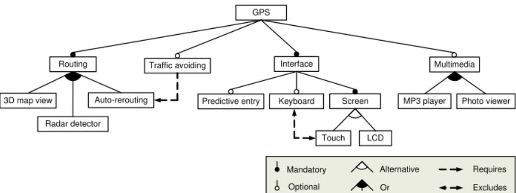
127
generated and therefore, as warned by software testing
128
experts, they are not sufficient to exercise the specific
129
features of a tool under evaluation. Another negative
130
consequence of using huge feature models to evaluate
131
the performance of tools is that they frequently fall out
132
of the scope of their users. Hence, both developers and
133
users would probably be more interested in knowing
134
whether a tool may crash with a hard model of small
135
or medium size.
136
Finally, we may mention that using realistic or
stan-137
dard collections of problems (i.e. benchmarks) is
138
equally insufficient for an exhaustive performance
uation since they do not consider the specific aspects
140
of a tool or technique under test. Thus, feature
mod-141
els that one tool finds hard to analyse could be trivially
142
processed by another and vice versa.
143
Solution overview and contributions. In this article,
144
we propose to model the problem of finding
computa-145
tionally hard feature models as an optimisation
prob-146
lem and we solve it using a novelEvolutionary
algo-147
riTHm for Optimised feature Models (ETHOM). Given
148
a tool and an analysis operation, ETHOM generates
in-149
put models of a predefined size maximising aspects such
150
as the execution time or the memory consumed by the
151
tool when performing the operation over the model. For
152
the evaluation of our approach, we performed several
153
experiments using different analysis operations, tools
154
and optimisation criteria. In particular, we used FaMa
155
and SPLOT, two tools for the automated analysis of
fea-156
ture models developed and maintained by independent
157
laboratories. In total, we performed over 50 million
158
executions of analysis operations for the configuration
159
and evaluation of our algorithm, during more than six
160
months of work. The results showed how ETHOM
suc-161
cessfully identified input models causing much longer
162
executions times and higher memory consumption than
163
randomly generated models of identical or even larger
164
size. As an example, we compared the effectiveness
165
of random and evolutionary search in generating
fea-166
ture models with up to 1,000 features maximising the
167
time required by a constraint programming solver (a.k.a.
168
CSP solver) to check their consistency. The results
re-169
vealed that the hardest randomly generated model found
170
required 0.2 seconds to analyse while ETHOM was able
171
to find several models taking between 1 and 27.5
min-172
utes to process. Besides this, we found that the
hard-173
est feature models generated by ETHOM in the range
174
500-1,000 features were remarkably harder to process
175
than randomly generated models with 10,000 features.
176
More importantly, we found that the hard feature
mod-177
els generated by ETHOM had similar properties to
re-178
alistic models found in the literature. This suggests that
179
the long execution times and high memory consumption
180
detected by ETHOM might be reproduced when using
181
real models with the consequent negative effect on the
182
user.
183
Our work enhances and complements the current
184
state of the art on performance evaluation of feature
185
model analysis tools as follows:
186
• To the best of our knowledge, this is the first
ap-187
proach that uses a search–based strategy to exploit
188
the internal weaknesses of the analysis tools and
189
techniques under evaluation rather than trying to
190
detect them by chance using randomly generated
191
models.
192
• Our work allows developers to focus on the search
193
for computationally hard models of realistic size
194
that could reveal performance problems in their
195
tools rather than using huge feature models out of
196
their scope. If a tool performs poorly with the
gen-197
erated models, developers could use the
informa-198
tion as input to investigate possible improvements.
199
• Our approach provides users with helpful
infor-200
mation about the behaviour of tools in pessimistic
201
cases helping them to choose the tool that best
202
meets their needs.
203
• Our algorithm is highly generic and can be applied
204
to any automated operation on feature models in
205
which the quality (i.e. fitness) of models with
re-206
spect to an optimisation criterion can be quantified.
207
• Our experimental results show that the hardness of
208
feature models depends on different factors in
con-209
trast to related work in which the complexity of the
210
models is mainly associated with their size.
211
• Our algorithm is ready-to-use and publicly
avail-212
able as a part of the open-source BeTTy
Frame-213
work [14, 58].
214
Scope of the contribution. The target audience of
215
this article is practitioners and researchers wanting to
216
evaluate and test the performance of their tools that
217
analyse feature models. Several aspects regarding the
218
scope of our contribution may be clarified, namely:
219
• Our work follows a black-box approach. That
220
is, our algorithm does not make any assumptions
221
about an analysis tool and operation under test.
222
ETHOM can therefore be applied to any tool or
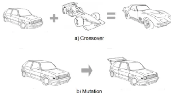
223
analysis operation regardless of how it is
imple-224
mented.
225
• Our approach focuses on testing, not debugging.
226
That is, our work contributes to the detection of
227
performance failures (unexpected behaviour in the
228
software) but not faults (causes of the unexpected
229
behaviour). Once a failure is detected using the
230
test data generated by ETHOM, a tool’s
develop-231
ers and designers should use debugging to identify
232
the fault causing it, e.g. bad variable ordering, bad
233
problem encoding, parsing problems, etc.
234
• It is noteworthy that many different factors could
235
contribute to a technique finding it hard to analyse
a given feature model, some of them not directly
237
related to the analysis algorithm used. Examples
238
including: bad variable ordering, bad problem
en-239
coding, parsing problems, bad heuristic selection,
240
etc. However, as previously mentioned, the
prob-241
lem of identifying the factors that make a feature
242
model hard to analyse when using a specific tool is
243
out of the scope of this article.
244
The rest of the article is structured as follows.
Sec-245
tion 2 introduces feature models and evolutionary
algo-246
rithms. In Section 3, we present ETHOM, an
evolu-247
tionary algorithm for the generation of optimised
fea-248
ture models. Then, in Section 4, we propose a specific
249
configuration of ETHOM to automate the generation
250
of computationally hard feature models. The
empiri-251
cal evaluation of our approach is presented in Section
252
5. Section 6 presents the threats to validity of our work.
253
Related work is described in Section 7. Finally, we
sum-254
marise our conclusions and describe our future work in
255
Section 8.
256
2. Preliminaries
257
2.1. Feature models and their analyses
258
Feature modelsdefine the valid combinations of
fea-259
tures in a domain and are commonly used as a compact
260
representations of all the products of an SPL. A feature
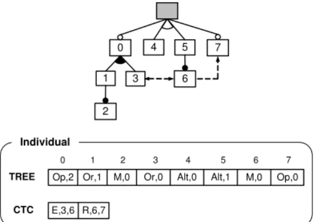
261
model is visually represented as a tree-like structure in
262
which nodes represent features and connections
illus-263
trate the relationships between them. These
relation-264
ships constrain the way in which features can be
com-265
bined. Fig. 1 depicts a simplified sample feature model.
266
The model illustrates how features are used to specify
267
and build software for Global Position System (GPS)
268
devices. The software loaded in the GPS is determined
269
by the features that it supports. The root feature (i.e.
270
‘GPS’) identifies the SPL.
271
Feature models were first introduced in 1990 as a
272
part of the FODA (Feature–Oriented Domain Analysis)
273
method [32]. Since then, feature modelling has been
274
widely adopted by the software product line community
275
and a number of extensions have been proposed in
at-276
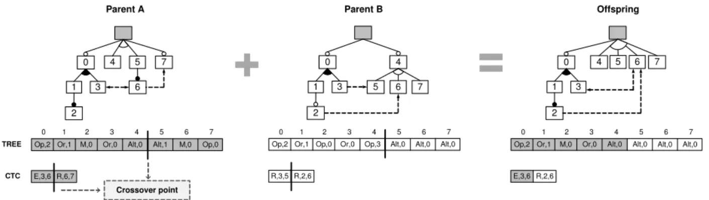
tempts to improve properties such as succinctness and
277
naturalness [56]. Nevertheless, there seems to be a
con-278
sensus that at a minimum feature models should be able
279
to represent the following relationships among features:
280
• Mandatory. If a child feature is mandatory, it is
281
included in all products in which its parent feature
282
appears. In Fig. 1, all GPS devices must provide
283
support forRouting.
284
• Optional. If a child feature is defined as optional,
285
it can be optionally included in products in which
286
its parent feature appears. For instance, the sample
287
model defines Multimedia to be an optional
fea-288
ture.
289
• Alternative. Child features are defined as
alter-290
native if only one feature can be selected when
291
the parent feature is part of the product. In our
292
SPL, software for GPS devices must provide
sup-293
port for either anLCDorTouchscreen but only one
294
of them.
295
• Or-Relation. Child features are said to have an
296
or-relation with their parent when one or more of
297
them can be included in the products in which the
298
parent feature appears. In our example, GPS
de-299
vices can provide support for an MP3 player, a
300
Photo vieweror both of them.
301
Notice that a child feature can only appear in a
prod-302
uct if its parent feature does. The root feature is a part
303
of all the products within the SPL. In addition to the
304
parental relationships between features, a feature model
305
can also containcross-tree constraintsbetween features.
306
These are typically of the form:
307
• Requires. If a feature A requires a feature B, the
308
inclusion of A in a product implies the inclusion of
309
B in the product. GPS devices withTraffic
avoid-310
ingrequireAuto-rerouting.
311
• Excludes.If a feature A excludes a feature B, both
312
features cannot be part of the same product. In our
313
sample SPL, a GPS withTouchscreen cannot
in-314
clude aKeyboardand vice-versa.
315
The automated analysis of feature models deals with
316
the computer-aided extraction of information from
fea-317
ture models. It has been noted that in the order of 30
dif-318
ferent analysis operations on feature models have been
319
reported during the last two decades [10]. The
analy-320
sis of feature models is usually performed in two steps.
321
First, the analysis problem is translated into an
interme-322
diate problem such as a boolean satisfiability problem
323
(SAT) or a Constraint Satisfaction Problem (CSP). SAT
324
problems are often modelled using Binary Decision
Di-325
agrams (BDD). Then, an off-the-shelf solver is used to
326
analyse the problem. Most analysis problems related to
327
feature models are NP-hard [7, 51]. However, solvers
328
provide heuristics that work well in practice.
Experi-329
ments have shown that each technique has its strengths
330
and weaknesses. For instance, SAT solvers are efficient
331
when checking the consistency of a feature model but
GPS Routing Interface MP3 player 3D map view Multimedia Screen LCD Touch Mandatory Optional Alternative Or Requires Excludes Photo viewer Traffic avoiding Radar detector
Auto-rerouting Predictive entry Keyboard
Figure 1: A sample feature model
incapable of calculating the number of products in a
333
reasonable amount of time [11, 45, 51]. BDD solvers
334
are the most efficient solution known for calculating the
335
number of products but at the price of high memory
con-336
sumption [11, 46, 51]. Finally, CSP solvers are
espe-337
cially suitable for dealing with numeric constraints
as-338
sociated with feature models with attributes (so-called
339
extended feature models) [9].
340
2.2. Evolutionary algorithms
341
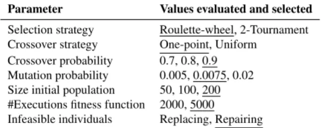
The principles of biological evolution have inspired
342
the development of a whole branch of optimisation
tech-343
niques calledEvolutionary Algorithms (EAs). These
al-344
gorithms manage a set of candidate solutions to an
opti-345
misation problem that are combined and modified
itera-346
tively to obtain better solutions. Each candidate solution
347
is referred to as anindividualorchromosomein analogy
348
to the evolution of species in biological genetics where
349
the DNA of individuals is combined and modified along
350
generations enhancing the species through natural
se-351
lection. Two of the main properties of EAs are that they
352
are heuristic and stochastic. The former means that an
353
EA is not guaranteed to obtain the global optimum for
354
the optimisation problem. The latter means that diff
er-355
ent executions of the algorithm with the same input
pa-356
rameters can produce different output, i.e. they are not
357
deterministic. Despite this, EAs are among the most
358
widely used optimisation techniques and have been
ap-359
plied successfully in nearly all scientific and
engineer-360
ing areas by thousands of practitioners. This success is
361
due to the ability of EAs to obtain near optimal
solu-362
tions to extremely hard optimisation problems with
af-363
fordable time and resources.
364
As an example, let us consider the design of a car as
365
an optimisation problem. A similar example was used
366
to illustrate the working of EAs in [73]. Let us suppose
367
that our goal is to find a car design that maximises
368
Initialization
Stop criteria met?
Selection Mutation Crossover Evaluation [NOT] [YES] Evaluation Encoding Decoding Survival
Figure 2: General working scheme of evolutionary algorithms
speed. This problem is hard since a car is a highly
369
complex system in which speed depends on a number
370
of parameters such as engine type and the shape of the
371
car. Moreover, there are likely to be extra constraints
372
like keeping the cost of the car under a certain value,
373
making some designs infeasible. All EA variants are
374
based on a common working scheme shown in Fig. 2.
375
Next, we describe its main steps and relate them to our
376
example.
377 378
Initialisation. The initial population (i.e. set of
379
candidate solutions to the problem) is usually generated
380
randomly. In our example, this could be done by
381
randomly choosing a set of values for the design
382
parameters of the car. Of course, it is unlikely that
383
this initial population with contain an optimal or
near optimal car design. However, promising
val-385
ues found at this step will be used to produce variants
386
along the optimisation process leading to better designs.
387 388
Evaluation. Next, individuals are evaluated using a
389
fitness function. A fitness function is a function that
390
receives an individual as input and returns a numerical
391
value indicating the quality of the individual. This
392
enables the objective comparison of candidate solutions
393
with respect to an optimisation problem. The fitness
394
function should be deterministic to avoid interferences
395
in the algorithm, i.e. different calls to the function with
396
the same set of parameters should produce the same
397
output. In our car example, a simulator could be used
398
to provide the maximum speed prediction as fitness.
399 400
Stopping criterion. Iterations of the remaining steps
401
of the algorithm are performed until a termination
cri-402
terion is met. Typical stopping criteria are: reaching a
403
maximum or average fitness value, maximum execution
404
times of the fitness function, number of iterations of
405
the loop (so-called generations) or number of iterations
406
without improvements on the best individual found.
407 408
Encoding. In order to create offspring, an individual
409
needs to beencoded(represented) in a form that
facili-410
tates its manipulation during the rest of the algorithm.
411
In biological genetics, DNA encodes an individual’s
412
characteristics on chromosomes that are used in
re-413
production and whose modifications produce mutants.
414
Classical encoding mechanisms for EAs include the
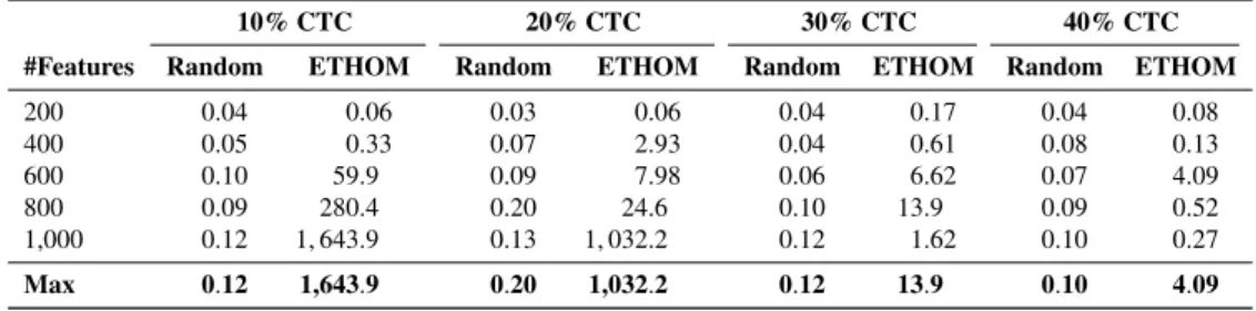
415
use of binary vectors that encode numerical values in
416
genetic algorithms (so-called binary encoding) and tree
417
structures that encode the abstract syntax of programs
418
in genetic programming (so-called tree encoding)
419
[1, 54]. In our car example, this step would require
420
design patterns of cars to be expressed using a data
421
structure, e.g. binary vectors for each design parameter.
422 423
Selection. In the main loop of the algorithm (see Fig.
424
2), individuals are selected from the current population
425
in order to create new offspring. In this process, better
426
individuals usually have a greater probability of being
427
selected, with this resembling natural evolution where
428
stronger individuals are more likely to reproduce. For
429
instance, two classic selection mechanisms are roulette
430
wheel and tournament selection [1]. When using the
431
former, the probability of choosing an individual is
432
proportional to its fitness and this can be seen as
deter-433
mining the width of the slice of a hypothetical spinning
434
roulette wheel. This mechanism is often modified
435
by assigning probabilities based on the position of
436
Figure 3: Sample crossover and mutation in the search of an optimal car design.
the individuals in a fitness–ordered ranking (so-called
437
rank-based roulette wheel). When using tournament
438
selection, a group of nindividuals is randomly chosen
439
from the population and a winning individual is selected
440
according to its fitness.
441 442
Crossover. These are the techniques used to combine
443
individuals and produce new individuals in an
analo-444
gous way to biological reproduction. The crossover
445
mechanism used depends on the encoding scheme but
446
there are a number of widely-used mechanisms [1].
447
For instance, two classical crossover mechanisms for
448
binary encoding are one-point crossover and uniform
449
crossover. When using the former, a location in the
450
vector is randomly chosen as the break point and
451
portions of vectors after the break point are exchanged
452
to produce offspring (see Fig. 5 for a graphical example
453
of this crossover mechanism). When using uniform
454
crossover, the value of each vector element is taken
455
from one parent or other with a certain probability,
456
usually 50%. Fig. 3(a) shows an illustrative application
457
of crossover in our example of car design. An F1
458
car and a small family car are combined by crossover
459
producing a sports car. The new vehicle has some
460
design parameters inherited directly from each parent
461
such as number of seats or engine type and others
462
mixed such as shape and intermediate size.
463 464
Mutation. At this step, random changes are applied to
465
the individuals. Changes are performed with a certain
466
probability where small modifications are more likely
467
than larger ones. Mutation plays the important role
468
of preventing the algorithm from getting stuck
prema-469
turely at a locally optimal solution. An example of
470
mutation in our car optimisation problem is presented
471
in Fig. 3(b). The shape of a family car is changed
472
by adding a back spoiler while the rest of its design
473
parameters remain intact.
474 475
Decoding. In order to evaluate the fitness of new
476
and modified individuals decoding is performed.
477
For instance, in our car design example, data stored
478
on data structures is transformed into a suitable car
479
design that our fitness function can evaluate. It often
480
happens that the changes performed in the crossover
481
and mutation steps create individuals that are not valid
482
designs or break a constraint, this is usually referred
483
to as an infeasible individual, e.g. a car with three
484
wheels. Once an infeasible individual is detected, this
485
can be either replaced by an extra correct one or it
486
can be repaired, i.e. slightly changed to make it feasible.
487 488
Survival. Finally, individuals are evaluated and the next
489
population is formed in which individuals with better
490
fitness values are more likely to remain in the
popula-491
tion. This process simulates the natural selection of the
492
better adapted individuals that survive and generate off
-493
spring, thus improving a species.
494
3. ETHOM: an Evolutionary algoriTHm for
Opti-495
mized feature Models
496
In this section, we present ETHOM, a novel
evo-497
lutionary algorithm for the generation of optimised
498
feature models. The algorithm takes several constraints
499
and a fitness function as input and returns a feature
500
model of the given size maximising the optimisation
501
criterion defined by the function. A key benefit of our
502
algorithm is that it is very generic and so is applicable
503
to any automated operation on feature models in which
504
the quality (i.e. fitness) of the models can be measured
505
quantitatively. In the following, we describe the basic
506
steps of ETHOM as shown in Fig. 2.
507 508
Initial population. The initial population is generated
509
randomly according to the size constraints received
510
as input. The current version of ETHOM allows the
511
user to specify the number of features, percentage of
512
cross-tree constraints and maximum branching factor of
513
the feature model to be generated. Several algorithms
514
for the random generation of feature models have been
515
proposed in the literature [57, 67, 78]. There are also
516
tools such as BeTTy [14, 58] and SPLOT [43, 65] that
517
support the random generation of feature models.
518 519
Evaluation. Feature models are evaluated according
520
to the fitness function received as input obtaining a
521
numeric value that represents the quality of a candidate
522
solution, i.e. its fitness.
523 524 0 2 1 3 4 5 6
Op,2 Or,1 M,0 Or,0 Alt,0 Alt,1 M,0
E,3,6 7 Op,0 R,6,7 TREE CTC Individual 0 1 2 3 4 5 6 7
Figure 4: Encoding of a feature model in ETHOM
Encoding. For the representation of feature models as
525
individuals (a.k.a. chromosomes) we propose using a
526
custom encoding. Generic encodings for evolutionary
527
algorithms were ruled out since these either were not
528
suitable for tree structures (i.e. binary encoding) or
529
were not able to produce solutions of a fixed size (e.g.
530
tree encoding), a key requirement in our approach. Fig.
531
4 depicts an example of our encoding. As illustrated,
532
each model is represented by means of two arrays,
533
one storing information about the tree and another one
534
containing information about Cross-Tree Constraints
535
(CTC). The order of each feature in the array
corre-536
sponds to the Depth–First Traversal (DFT) order of
537
the tree. Hence, a feature labelled with‘0’ in the tree
538
is stored in the first position of the array, the feature
539
labelled with ‘1’ is stored the second position and so
540
on. Each feature in the tree array is defined by a pair
541
< PR,C >wherePR is the type of relationship with
542
its parent feature (M: Mandatory, Op: Optional, Or:
543
Or-relationship, Alt: Alternative) andC is the number
544
of children of the given feature. As an example, the
545
first position in the tree array,<Op,2>, indicates that
546
the feature labelled with‘0’in the tree has an optional
547
relationship with its parent feature and has two child
548
features (those labelled with‘1’and‘3’). Analogously,
549
each position in the CTC array stores information about
550
one constraint in the form< T C,O,D >whereTC is
551
the type of constraint (R: Requires, E: Excludes) and
552
O andD are the indexes of the origin and destination
553
features in the tree array respectively.
554 555
Selection. Selection strategies are generic and can
556
be applied regardless of how the individuals are
557
represented. In our algorithm, we implemented both
558
rank-based roulette-wheel and binary tournament
559
selection strategies. The selection of one or the other
E,3,6
Op,2 Or,1 M,0 Or,0 Alt,0
E,3,6 R,6,7
M,0 Or,0 Alt,0 Alt,1 M,0 Op,0 Op,2 Or,1 0 2 1 3 4 5 6 7 TREE CTC 0 2 1 3 5 6 7
Op,2 Or,1 Op,0 Or,0 Op,3 Alt,0 Alt,0
R,3,5 4 Alt,0 R,2,6 0 2 1 3 5 6 4
Alt,0 Alt,0 Alt,0
R,2,6
7
Parent A Parent B Offspring
Crossover point
0 1 2 3 4 5 6 7 0 1 2 3 4 5 6 7 0 1 2 3 4 5 6 7
Figure 5: Example of one-point crossover in ETHOM
mainly depends on the application domain.
561 562
Crossover. We provided our algorithm with two
563
different crossover techniques, one-point and uniform
564
crossover. Fig. 5 depicts an example of the application
565
of one-point crossover in ETHOM. The process starts
566
by selecting two parent chromosomes to be combined.
567
For each array in the chromosomes, the tree and
568
CTC arrays, a random point is chosen (the so-called
569
crossover point). Finally, the offspring is created by
570
copying the contents of the arrays from the beginning
571
to the crossover point from one parent and the rest from
572
the other one. Notice that the characteristics of our
573
encoding guarantee a fixed size for the individuals in
574
terms of features and CTCs.
575 576
Mutation.Mutation operators must be specifically
de-577
signed for the type of encoding used. ETHOM uses four
578
different types of custom mutation operators, namely:
579
• Operator 1. This randomly changes the type
580
of a relationship in the tree array, e.g. from
581
mandatory,<M,3>, to optional,<Op,3>.
582
• Operator 2.This randomly changes the number of
583
children of a feature in the tree, e.g. from<M,3>
584
to<M,5>. The new number of children is in the
585
range [0,BF] whereBFis the maximum branching
586
factor indicated as input.
587
• Operator 3. This changes the type of a cross-tree
588
constraint in the CTC array, e.g. from excludes
589
<E,3,6>to requires<R,3,6>.
590
• Operator 4. This randomly changes (with equal
591
probability) the origin or destination feature of a
592
constraint in the CTC array, e.g. from<E,3,6 >
593
to<E,1,6>. The implementation of this ensures
594
that the origin and destination features are diff
er-595
ent.
596
These operators are applied randomly with the same
597
probability.
598 599
Decoding. At this stage, the array-based chromosomes
600
are translated back into feature models so that they
601
can be evaluated. In ETHOM, we identified three
602
types of patterns making a chromosome infeasible or
603
semantically redundant, namely: i) those encoding set
604
relationships (or- and alternative) with a single child
605
feature (e.g. Fig. 6(a)),ii) those containing cross-tree
606
constraints between features with parental relationship
607
(e.g. Fig. 6(b)), andiii) those containing features linked
608
by contradictory or redundant cross-tree constraints
609
(e.g. Fig. 6(c)). The specific approach used to address
610
infeasible individuals, replacing or repairing (see
611
Section 2.2 for details), mainly depends on the problem
612
and it is ultimately up to the user. In our work, we used
613
a repairing strategy described in the next section.
614 615 B A B A B A B A A B B A B A B A B A (a) (d) (b) (e) (c) (f) In c o n s is te n c y R e p a ir
Figure 6: Examples of infeasible individuals and repairs
Survival. Finally, the next population is created by
616
including all the new offspring plus those individuals
from the previous generation that were selected for
618
crossover but did not generate descendants.
619 620
For a pseudo-code listing of the algorithm we refer
621
the reader to [59].
622
4. Automated generation of hard feature models
623
In this section we propose a method that models the
624
problem of finding computationally hard feature
mod-625
els as an optimisation problem and explain how this is
626
solved using ETHOM. In order to find a suitable
con-627
figuration of ETHOM, we performed numerous
execu-628
tions of a sample optimisation problem evaluating
dif-629
ferent combination of values for the key parameters of
630
the algorithm, presented in Table 1. The optimisation
631
problem was to find a feature model maximising the
632
execution time taken by the analysis tool when
check-633
ing model consistency, i.e. whether it represents at least
634
one product. We chose this analysis operation because
635
it is currently the most frequently quoted in the
litera-636
ture [10]. In particular, we searched for feature models
637
of different size maximising execution time in the CSP
638
solver JaCoP [29] integrated into the framework for the
639
analysis of feature models FaMa [19]. Next, we clarify
640
the main aspects of the configuration of ETHOM:
641
• Initial population. We used a Java program
im-642
plementing the algorithm for the random
genera-643
tion of feature models described by Th¨um et al.
644
[67]. For a detailed description of the generation
645
approach, we refer the reader to [59].
646
• Fitness function. Our first attempt was to
mea-647
sure the time (in milliseconds) taken by FaMa to
648
perform the operation. However, we found that
649
the result of the function was significantly affected
650
by the system load and was not deterministic. To
651
solve this problem, we decided to measure the
fit-652
ness of a feature model as the number of
back-653
tracks produced by the analysis tool during its
anal-654
ysis. Abacktrackrepresents a partial candidate
so-655
lution to a problem that is discarded because it
can-656
not be extended to a full valid solution [68]. In
con-657
trast to the execution time, most CSP backtracking
658
heuristics are deterministic, i.e. different
execu-659
tions of the tool with the same input produce the
660
same number of backtracks. Together with
execu-661
tion time, the number of backtracks is commonly
662
used to measure the complexity of constraint
satis-663
faction problems [68]. Thus, we can assume that
664
the higher the number of backtracks the longer the
665
computation time.
666
• Infeasible individuals. We evaluated the eff
ec-667
tiveness of both replacement and repair techniques.
668
More specifically, we evaluated the following
re-669
pair algorithm applied to infeasible individuals: i)
670
isolated set relationships are converted into
op-671
tional relationships (e.g. the model in Fig. 6(a) is
672
changed as in Fig. 6(d)),ii) cross-tree constraints
673
between features with parental relationships are
re-674
moved (e.g. the model in Fig. 6(b) is changed as in
675
Fig. 6(e)), andiii) two features cannot be linked by
676
more than one cross-tree constraint (e.g. the model
677
in Fig. 6(c) is changed as in Fig. 6(f)).
678
• Stopping criterion. There is no means of
decid-679
ing when an optimum input has been found and
680
ETHOM should be stopped [73]. For the
config-681
uration of ETHOM, we decided to allow the
al-682
gorithm to continue for a given number of
execu-683
tions of the fitness function (i.e. maximum number
684
of generations) taking the largest number of
back-685
tracks obtained as the optimum, i.e. the solution to
686
the problem.
687
Table 1 depicts the values evaluated for each
config-688
uration parameter of ETHOM. These values were based
689
on related work using evolutionary algorithms [23], the
690
literature on parameter setting [18], and our previous
691
experience in this domain [48]. Each combination of
692
parameters used was executed 10 times to avoid
hetero-693
geneous results and to allow us to perform statistical
694
analysis on the data. The values underlined are those
695
that provided better results and were therefore selected
696
for the final configuration of ETHOM. In total, we
per-697
formed over 40 million executions of the objective
func-698
tion to find a good setup for our algorithm.
699
Parameter Values evaluated and selected
Selection strategy Roulette-wheel, 2-Tournament
Crossover strategy One-point, Uniform
Crossover probability 0.7, 0.8, 0.9
Mutation probability 0.005, 0.0075, 0.02
Size initial population 50, 100, 200
#Executions fitness function 2000, 5000
Infeasible individuals Replacing, Repairing
Table 1: ETHOM configuration
5. Evaluation
700
In order to evaluate our approach, we developed a
701
prototype implementation of ETHOM. The prototype
702
was implemented in Java to facilitate its integration into
the BeTTy Framework [14, 58], an open-source Java
704
tool for functional and performance testing of tools that
705
analyse feature models1. 706
We evaluated the efficacy of our approach by
compar-707
ing it to random search since this is the usual approach
708
for performance testing in the analysis of feature
mod-709
els. In particular, the evaluation of our evolutionary
pro-710
gram was performed through a number of experiments.
711
In each experiment, we compared the effectiveness of
712
a random generator and ETHOM when searching for
713
feature models maximising properties such as the
exe-714
cution time or memory consumption required for their
715
analysis. Additionally, we performed some extra
exper-716
iments studying the characteristics of the hard feature
717
models generated and the behaviour of ETHOM when
718
allowed to run for a large number of generations. The
719
setup and results of our experiments as well as the
statis-720
tical analysis of the data are summarised in this section
721
and fully reported in an external technical report due
722
to space limitations [59]. The experimental work and
723
the statistical analysis of the results took more than six
724
months and involved several people.
725
All the experiments were performed on a cluster of
726
four virtual machines equipped with an Intel Core 2
727
CPU [email protected] running Centos OS 5.5 and Java
728
1.6.0 20 on 1400 MB of dedicated memory. These
vir-729
tual machines ran on a cloud of servers equipped with
730
Intel Core 2 CPU [email protected] and 4GB of RAM
731
memory managed using Opennebula 2.0.1.
732
5.1. Experiment #1: Maximizing execution time in a
733
CSP solver
734
This experiment evaluated the ability of ETHOM
735
to search for input feature models maximising the
736
analysis time of a solver. In particular, we measured the
737
execution time required by a CSP solver to determine
738
whether the input model was consistent (i.e. it
repre-739
sents at least one product). This was the problem used
740
to tune the configuration of our algorithm. Again, we
741
chose the consistency operation because currently it is
742
the most frequently mentioned in the literature. Next,
743
we present the setup and results of our experiment.
744 745
Experimental setup. This experiment was performed
746
through a number of iterative steps. In each step, we
747
randomly generated 5,000 feature models and checked
748
their consistency, saving the maximum fitness obtained.
749
Then, we executed ETHOM and allowed it to run for
750
the same number of executions of the fitness function
751
1BeTTY was used because it was developed by the authors
(5,000) and compared the results. Recall that the size
752
of the population in our algorithm was set to 200
753
individuals which meant that the maximum number
754
of generations was 25, i.e. 5,000/200. This process
755
was repeated with different model sizes to evaluate the
756
scalability of our algorithm. In particular, we generated
757
models with different combinations of features, {200,
758
400, 600, 800, 1,000} and percentage of constraints
759
(with respect to the number of features), {10%, 20%,
760
30%, 40%}. The maximum branching factor was set
761
to 10 in all the experiments. For each model size,
762
we repeated the process 25 times to get averages and
763
performed statistical analysis on the data. In total, we
764
performed about 5 million executions2 of the fitness
765
function for this experiment. The fitness was set to
766
be the number of backtracks used by the analysis tool
767
when checking the model consistency. For the analysis,
768
we used the solver JaCoP integrated into FaMa v1.0
769
with the default heuristics MostConstrainedDynamic
770
for the selection of variables and IndomainMinfor the
771
selection of values from the domains. To prevent the
772
experiment from getting stuck, a maximum timeout of
773
30 minutes was used for the execution of the fitness
774
function in both the random and evolutionary search. If
775
this timeout was exceeded during random generation,
776
the execution was cancelled and a new iteration was
777
started. If the timeout was exceeded during
evolution-778
ary search, the best solution found until that moment
779
was returned, i.e. the instance exceeding the timeout
780
was discarded. After all the executions, we measured
781
the execution time of the hardest feature models found
782
for a full comparison, i.e. those producing a larger
783
number of backtracks. More specifically, we executed
784
each returned solution 10 times to get average execution
785
times.
786 787
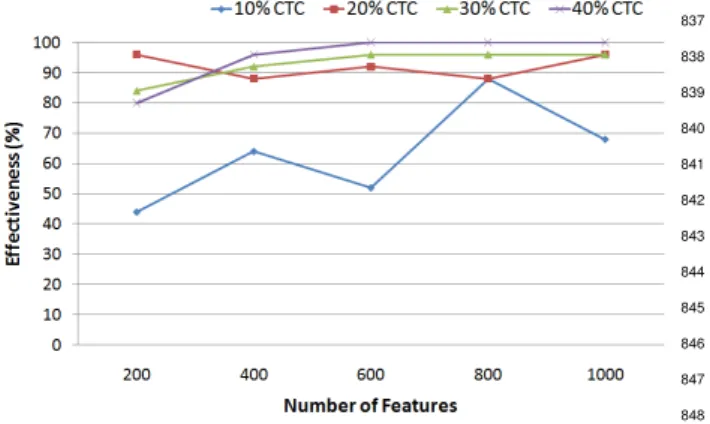
Analysis of results. Fig. 7 depicts the effectiveness of
788
ETHOM for each size range of the feature models
gen-789
erated. We define theeffectivenessof our evolutionary
790
program as the percentage of times (out of 25) in which
791
ETHOM found a better optimum than random search,
792
i.e. a higher number of backtracks. As illustrated, the
793
effectiveness of ETHOM was over 80% in most of the
794
size ranges, reaching 96% or higher in nine of them.
795
Overall, our evolutionary program found harder feature
796
models than those generated randomly in 85.8% of the
797
executions. We may remark that our algorithm revealed
798
the lowest effectiveness with those models containing
799
10% of cross-tree constraints. We found that this was
800
25 features ranges x 4 constraints ranges x 25 iterations x 10,000 (5,000 random search+5,000 evolutionary search)
Figure 7: Effectiveness of ETHOM in Experiment #1.
due to the simplicity of the analysis in this size range.
801
The number of backtracks produced by these models
802
was very low, zero in most cases, and thus ETHOM
803
had problems finding promising individuals that could
804
evolve towards optimal solutions.
805
Table 2 depicts the evaluation results for the range of
806
feature models with 20% of cross-tree constraints. For
807
each number of features and search technique, random
808
and evolutionary, the table shows the average and
max-809
imum fitness obtained (i.e. number of backtracks) as
810
well as the average and maximum execution times of the
811
hardest feature models found (in seconds). The eff
ec-812
tiveness of the evolutionary program is also presented
813
in the last column. As illustrated, ETHOM found
fea-814
ture models producing a number of backtracks larger by
815
several orders of magnitude than those produced using
816
randomly generated models. The fitness of the hardest
817
models generated using our evolutionary approach was
818
on average over 3,500 times higher than that of
ran-819
domly generated models (200,668 backtracks against
820
45.3) and 40,500 times higher in the maximum value
821
(23.5 million backtracks against 1,279). As expected,
822
these results were also reflected in the execution times.
823
On average, the CSP solver took 0.06 seconds to
anal-824
yse the randomly generated models and 9 seconds to
825
analyse those generated using ETHOM. The
superior-826
ity of evolutionary search was remarkable in the
maxi-827
mum times ranging from the 0.2 seconds for randomly
828
generated models to the 1,032.2 seconds (17.2 minutes)
829
taken by the CSP solver to analyse the hardest feature
830
model generated by ETHOM. Overall, our
evolution-831
ary approach produced a harder feature model than
ran-832
dom techniques in 92% of the executions in the range of
833
20% of constraints. For details regarding the data
corre-834
sponding to 10%, 30% and 40% of constraints we refer
835
the reader to [59].
836
Table 3 presents a summary of the results. The
ta-837
ble depicts the maximum execution time taken by the
838
CSP solver to analyse the hardest models found
us-839
ing random and evolutionary search. The data shows
840
that ETHOM found models that led to higher execution
841
times than those randomly generated and this was the
842
case for all size ranges. The hardest randomly generated
843
model required 0.2 seconds to be processed. In contrast,
844
ETHOM found four models whose analysis required
be-845
tween 1 and 27.3 minutes (1,644 seconds). We may
846
remark that ETHOM reached the maximum timeout
847
of 30 minutes once during the experiment but random
848
search never produced times over 0.2 seconds.
Interest-849
ingly, ETHOM was able to find smaller but significantly
850
harder feature models (e.g. 600-10%, 60 seconds) than
851
the hardest randomly generated model found which had
852
800 features, 20% of CTCs and an analysis time of 0.2
853
seconds. Finally, the results show that ETHOM found
854
it more difficult to find hard feature models as the
per-855
centage of cross-tree constraints increased. We remark,
856
however, that this trend was also observed in the random
857
search with an average fitness of 45.3 backtracks in the
858
range of 20% CTC, 16.6 backtracks in the range of 30%
859
CTC and 9.1 backtracks in the range of 40% CTC. We
860
conclude, therefore, that these results are caused by the
861
CSP solver and the heuristic used which provide a better
862
performance when the models have a high percentage of
863
constraints.
864
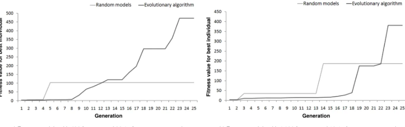
Fig. 8 compares random and evolutionary techniques
865
for the search for a feature model maximising the
num-866
ber of backtracks in two sample executions.
Horizon-867
tally, the graphs show the number of generations where
868
each generation represents 200 executions of the fitness
869
function. Fig. 8(a) shows that random search reaches
870
its maximum number of backtracks after only 5
gen-871
erations (about 1000 executions). That is, the random
872
generation of 4,000 other models does not produce any
873
higher number of backtracks and therefore is useless. In
874
contrast to this, ETHOM shows a continuous
improve-875
ment. After 13 generations (about 2600 executions),
876
the fitness found by evolutionary search is above that of
877
the maximum for the randomly generated models. Fig.
878
8(b) depicts another example in which random search
879
is ‘lucky’ and finds an instance with a high number of
880
backtracks in the 14th generation. Evolutionary
optimi-881
sation, however, once again manages to improve the
ex-882
ecution times continuously overcoming the best fitness
883
produced using random search after 22 generations. We
884
might note that a significant leap of about 200
back-885
tracks can also be observed in generation 23. In both
886
examples, the curve suggests that ETHOM would find
887
even better solutions if the number of generations was
Random Search ETHOM
#Features Avg Fitness Max Fitness Avg Time Max Time Avg Fitness Max Fitness Avg Time Max Time Effect. (%)
200 8.08 61 0.02 0.03 63.4 215 0.04 0.06 96 400 30.1 389 0.04 0.07 7,128.4 106,655 0.24 2.93 88 600 40.3 477 0.05 0.09 9,188.2 116,479 0.70 7.98 92 800 91.1 1,279 0.08 0.20 22,427.6 483,971 1.28 24.6 88 1000 57.2 582 0.10 0.13 964,532.6 23,598,675 42.5 1,032.2 96 Total 45.3 1,279 0.06 0.20 200,668 23,598,675 8.96 1,032.2 92
Table 2: Evaluation results on the generation of feature models maximising execution time in a CSP solver. Fitness measured in number of backtracks. Time in seconds. CTC=20%
10% CTC 20% CTC 30% CTC 40% CTC
#Features Random ETHOM Random ETHOM Random ETHOM Random ETHOM
200 0.04 0.06 0.03 0.06 0.04 0.17 0.04 0.08 400 0.05 0.33 0.07 2.93 0.04 0.61 0.08 0.13 600 0.10 59.9 0.09 7.98 0.06 6.62 0.07 4.09 800 0.09 280.4 0.20 24.6 0.10 13.9 0.09 0.52 1,000 0.12 1,643.9 0.13 1,032.2 0.12 1.62 0.10 0.27 Max 0.12 1,643.9 0.20 1,032.2 0.12 13.9 0.10 4.09
Table 3: Maximum execution times produced by random and evolutionary search. Time in seconds.
increased. This was confirmed in a later experiment in
889
which the program was allowed to run for up to 125
890
generations (25,000 executions of the fitness function)
891
finding feature models producing more than 77.6
mil-892
lion backtracks (see Section 5.3 for details).
893
5.2. Experiment #2: Maximizing memory consumption
894
in a BDD solver
895
This experiment evaluated the ability of ETHOM to
896
generate input feature models maximising the memory
897
consumption of a solver. In particular, we measured the
898
memory consumed by a BDD solver when determining
899
the number of products represented by the model. We
900
chose this analysis because it is one of the hardest
901
operations in terms of complexity and it is the second
902
most frequently quoted operation in the literature [10].
903
We decided to use a BDD-based reasoner for this
904
experiment since it has proved to be the most efficient
905
option to perform this operation in terms of time
906
[10, 51]. ABinary Decision Diagram(BDD) solver is
907
a software package that takes a propositional formula
908
as input and translates it into a graph representation
909
(the BDD itself) that provides efficient algorithms for
910
counting the number of possible solutions. The number
911
of nodes of the BDD is a key aspect since it determines
912
the consumption of memory and can be exponential
913
in the worst case [46]. Next, we present the setup and
914
results of our experiment.
915 916
Experimental setup. The experiment consisted of a
917
number of iterative steps. At each step, we randomly
918
generated 5,000 models and compiled each of them
919
into a BDD for use in counting the number of solutions
920
of the input feature model. We then executed ETHOM
921
and allowed it to run for 5,000 executions of the fitness
922
function (i.e. 25 generations) searching for feature
923
models maximising the size of the BDD. Again, this
924
process was repeated with different combinations of
925
features, {50, 100, 150, 200, 250}and percentages of
926
constraints,{10%, 20%, 30%}to evaluate the scalability
927
of our approach. For each model size, we repeated
928
the process 25 times to get statistics from the data.
929
In total, we performed about 3.5 million executions
930
of the fitness function for this experiment. We may
931
remark that we generated smaller feature models than
932
those presented in the previous experiment in order to
933
reduce BDD building time and make the experiment
934
affordable. Measuring memory usage in Java is difficult
935
and computationally expensive since memory profilers
936
usually add a significant overload to the system. To
937
simplify the fitness function, we decided to measure the
938
fitness of a model as the number of nodes of the BDD
939
representing it. This is a natural option used in the
940
research community to compare the space complexity
941
of BDD tools and heuristics [46]. For the analysis,
942
we used the solver JavaBDD [30] integrated into the
943
feature model analysis tool SPLOT [43]. We chose
944
SPLOT for this experiment because it integrates highly
a) Feature models with 400 features and 30% of cross-tree constraints b) Feature models with 1,000 features and 10% of cross-tree constraints Generation Generation F it n e s s v a lu e f o r b e s t in d iv id u a l F it n e s s v a lu e f o r b e s t in d iv id u a l
Figure 8: Comparison of randomly generated models and ETHOM for the search of the highest number of backtracks
efficient ordering heuristics specifically designed for the
946
analysis of feature models using BDDs. In particular,
947
we used the heuristic ‘Pre-CL-MinSpan’presented by
948
Mendonca et al. in [46]. For a detailed description of
949
the configuration of the solver we refer the reader to
950
[59]. As in our previous experiment, we set a maximum
951
timeout of 30 minutes for the fitness function to prevent
952
the experiment from getting stuck. We measured the
953
compilation and execution time of the hardest feature
954
models found to allow a more detailed comparison.
955
Each optimal solution was compiled and executed 10
956
times to get average times.
957 958
Analysis of results. Fig. 9 depicts the effectiveness of
959
ETHOM for each size range of the feature models
gen-960
erated, i.e. percentage of times (out of 25) in which
evo-961
lutionary search found feature models producing higher
962
memory consumption than randomly generated
mod-963
els. As illustrated, the effectiveness of ETHOM was
964
over 96% in most cases, reaching 100% in 10 out of
965
the 15 size ranges. The lowest percentages were
regis-966
tered in the range of 250 features. When analysing the
967
results, we found that the timeout of 30 minutes was
968
reached frequently in the range of 250 features
hinder-969
ing ETHOM from evolving toward promising solutions.
970
In other words, the feature models generated were so
971
hard that they often took more than 30 minutes to
anal-972
yse and were discarded. In fact, the maximum
time-973
out was reached 18 times during random generation and
974
62 times during evolutionary search, 25 of them in the
975
range of 250 features and 30% of constraints. In this
976
size range, ETHOM exceeded the timeout after only 7
977
generations on average (25 being the maximum).
Over-978
all, ETHOM found feature models producing higher
979
memory consumption than random search in 94.4% of
980
the executions. The results suggest, however, that
in-981
Figure 9: Effectiveness of ETHOM in Experiment #2.
creasing the maximum timeout would significantly
im-982
prove the effectiveness.
983
Table 4 depicts the number of BDD nodes of the
hard-984
est feature models found using random and
evolution-985
ary search. For each size range, the table also shows
986
the computation time (BDD building time+execution
987
time) taken by SPLOT to analyse the model. As
il-988
lustrated, ETHOM found higher maximum values than
989
random techniques in all size ranges. On average, the
990
BDD size found by our evolutionary approach was
be-991
tween 1.03 and 10.3 times higher than those obtained
992
with random search. The largest BDD generated in
ran-993
dom search had 14.8 million nodes while the largest
994
BDD obtained using ETHOM had 20.6 million nodes.
995
Again, the results revealed that ETHOM was able to
996
find smaller but harder models (e.g. 150-30%, 17.7
mil-997
lion nodes) than the hardest randomly generated model
998
found, 250-30% 14.8 million nodes. We may recall that
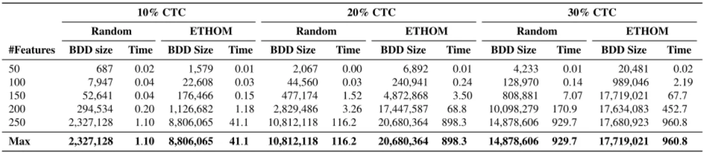
999
the maximum timeout was reached 62 times during the
1000
execution of ETHOM. This result suggests that the
max-1001
imum found by evolutionary search would have been