A WEB-BASED DSS ARCHITECTURE AND ITS
FORECASTING CORE IN SUPPLY CHAIN MANAGEMENT
Tien-You Wang
*and Din-Horng Yeh
*
Department of International Business Management
Tainan University of Technology
Tainan (710), Taiwan
Department of Business Administration
National Chung Cheng University
Chiayi (621), Taiwan
ABSTRACT
In a competitive market environment, supply chain management (SCM) has been critical for companies to survive. Demand planning plays an important role in SCM, for it provides accurate demand forecasts which may achieve customer satisfaction by offering benefits such as low inventory level, short lead time, efficient resource allocation, and quick response. To obtain more accurate forecasts, this study presents a web-based Decision Support System (DSS) architecture and its forecasting core. The forecasting core, named Panel Function, contains three modules: Segmentation Module, Forecasting Module, and Coordination Module. The Segmentation Module categorizes customers into three segments: Loyal Customer Segment, Potential Customer Segment, and Switcher Segment. Based on the three segments, the Forecasting Module employs different forecasting and analysis technologies to make an integrated forecast estimate: time-series forecasting to capture the loyal customer demand trend, Bayesian inference to estimate the predicted value of switcher purchase quantity, and questionnaire analysis and brand choice models to unearth potential customers. The results from these three processes are then synthesized to obtain the integrated forecast, which is then used in the Coordination Module as the base of distribution planning, and provides a minimal system-wide total cost solution for all parties in the supply chain. As a whole, this DSS architecture has been shown to provide an efficient mechanism for collaborative demand planning and help create the maximum profit for the supply chain.
Keywords: Web-based DSS, Forecasting, Purchase Tendency, Integrated Forecast, Data Mining
* Corresponding author: [email protected]
1. INTRODUCTION
Supply chain management (SCM), a hot business issue for the recent decade, has been granted as the solution of survival in current competitive market environment. Many companies recognize the importance of SCM in order to remain competitive, but the implementation of SCM seems no easy task to be accomplished. According to a Deloitte Consulting survey in 1998, about 91% of North American manufacturers rank SCM as very important or critical to their company's success. However, only 2% of them in the same survey rank their supply chains as world class [26].
The main reason for this extreme disparity might be the complexity of integrating logistics
operations among firms as well as within firm boundaries while bringing to bear appropriate information technologies [21]. Many researches point out that firms were confronted with various obstacles of employing SCM, some of them involve cost of communication with and coordination among different suppliers [2], high costs of the investment in employing information systems and developing the information technology (IT) skills of their employees [5], and the complex relationships in a supply chain, etc.
The participants in a supply chain form an alliance that can quickly bring together a set of core competencies to take advantage of a market opportunity. This leads to the advantages of adaptability, flexibility, agility, ability to globalize,
and allowing partner firms to concentrate on their core competence [25]. This alliance requires timely availability of information throughout the supply chain to allow cooperative and synchronized flow of material, products, and information among all participants [3]. However, exhaustive collaboration is required in such an environment, managers are often reluctant to devote themselves to a virtual team because they might lose control of proprietary information and technology, and they also have to trust outsiders and do much more negotiation as well as coordination [25]. These difficulties in SCM may possibly account for the phenomenon of the well-known bullwhip effect.
The bullwhip effect happens when the demand information moving upstream in a supply chain is distorted and amplified. Lee et al. [13] identified one of the main causes to be demand forecast updating. They contended that demand signal processing (implicating information delays) was a major contributor to the bullwhip effect, which leads to serious inventory problems. Lee et al. [13] pointed out that one remedy was to make demand data at a downstream site available to the upstream site, so that both sites could update their forecasts with the same raw data. Nevertheless, even though the demand data are shared with both upstream and downstream sites, the inaccurate forecasts led by limitations of current forecasting technologies still remain as a major problem of inventory in SCM.
To minimize the bullwhip effect, demand forecasting plays an important role in SCM. Accurate demand forecasts may achieve customer satisfaction by offering benefits such as low inventory level, short lead time, efficient resource allocation, and quick response. However, the performance of demand forecasting has been staggering due to the changing market environment and the limitation of existing forecasting technologies. This study attempts to improve forecasting performance and to facilitate collaborative forecasting in a supply chain by presenting a web-based DSS architecture with an integrated forecasting core in it. The forecasting core separates customers into three segments: Loyal Customer Segment, Switcher Segment, and Potential Customer Segment. Different technologies are employed in these three segments according to their characteristics. The results from these three segments are integrated to obtain the forecast, which is anticipated to attenuate the forecasting error. Section 2 illustrates these technologies and related researches, Section 3 depicts the details of the presented DSS architecture, Section 4 describes the forecasting core, Section 5 lists the implementation results, and Section 6 provides the discussion and conclusion.
2. APPLICATIONS OF RELATED
TECHNOLOGIES
The technologies involved in the presented DSS architecture consist of different domains, including decision support system, time-series forecasting, Bayesian inference, and brand choice models. These technologies and some of their applications are illustrated as follows.
2.1 Decision Support System (DSS)
DSS technology has been rising and flourishing since 1970s. Shim et al. [24] presented the evolution and categories of DSS, including data warehousing, OLAP, data mining, web-based DSS, collaborative support systems, and optimization- based DSS. A web-based DSS refers to a computerized system that delivers decision support information through a web browser to someone who needs it. When a user sends requests on a website, this system passes the requests to a database server which generates the query result set and sends it back for viewing. The web-based DSS serves incessantly with data warehouses and OLAP, but web database architecture should be able to handle a large number of concurrent requests when the number of users increases. The web environment is emerging as a very important platform for DSS development, using a web infrastructure for building DSS improves the rapid dissemination of decision-making frameworks and promotes more consistent decision making on repetitive tasks. This may help facilitate collaboration between the supply chain members, so the web-based DSS is chosen as the DSS architecture.
2.2 Forecasting
Current forecasting technologies refer to quantitative and qualitative methods. Among the quantitative methods, time-series forecasting methods are used to analyze time-dependent series data and predict the future values, brand choice models are used to calculate the probability of choice to predict choice behavior, and Bayesian models are used to infer conditional probability. Qualitative forecasting technology can be described by environment scanning, scenarios, and Delphi. A review of recent advances in technological forecasting can be found in Martino [19]. The forecasting technologies in the presented architecture focus on quantitative methods. 2.2.1 Time-series Forecasting
Time-series forecasting performs linear analysis on demand data to calculate forecasts. Benchmark methods in this domain include moving average, exponential smoothing, and autoregressive integrated moving average (ARIMA). Among these models,
ARIMA yields minimal mean square error [1], this makes it the typical method for time-series forecasting. In using time-series forecasting methods, forecasters assume that the past of a time series contains all the information needed to predict the future of that time series. An appropriate model is then fitted to the historical data, and the projection of that model becomes the forecast. This assumption implies the neglect of exploring the influences from environmental changes and customer purchase preference, which induces a lagging forecast with elusive residual error. Another limitation of time-series forecasting technology is that when it performs on nonlinear time series, the error caused by unknown factors remains to be solved. Recent researchers on time-series forecasting try to help solve this problem by employing heuristic methods such as data mining to capture the demand patterns inherent in nonlinear time series [4,9,12,22,27]. A survey of time-series data mining was presented by Keogh & Kasetty [10]. Although some accomplishment have been achieved by the effort, in general difficulties still remain because uncertain demand variations do not follow the same pattern all the time due to consumer behavior, new technologies or products, and other environmental factors. Exploring the composite effects of these factors that influence customer demand may capture the future trend and help reduce the errors that might exist in classical time-series forecasting models.
2.3 Segmentation with Data Mining
The diversity of customer purchase behavior contributes to the demand variation significantly in retailing industry, so customer purchase tendency is selected for exploring a forecasting alternative that is distinguished from traditional time-series technologies. From the viewpoint of resource allocation, retail management should prioritize customers in the following order: (1) existing loyal customers, (2) new entrants to the market, and (3) shoppers who are potentially switchable from competitors [23]. Based on this viewpoint, customers are classified into three segments: Loyal Customer Segment, Potential Customer Segment, and Switcher Segment in this study. The “Loyal Customer” purchases the product constantly; the “Switcher” purchases only at premium prices, and the "Potential Customer" has never purchased the specific product but there is a high possibility of purchasing it in the future.
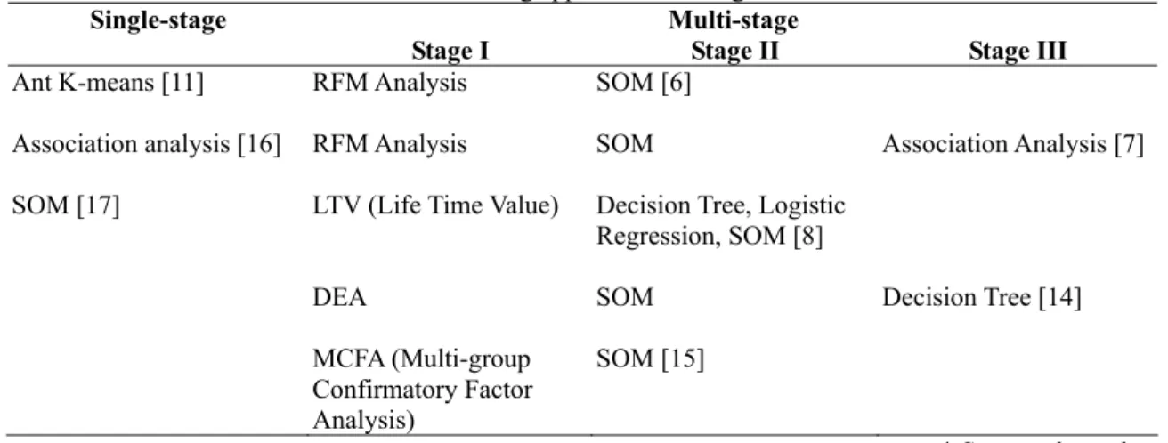
Classical segmentation methods refer to qualitative approach such as Recency, Frequency, and Monetary (RFM) analysis, or quantitative approach such as K-means. In recent years data mining has received more attention from researchers who work on segmentation. Some of them employ multi-stage procedure by integrating classical segmentation methods with data mining technology, while others take one of the data mining methods as the major approach. The methods used in the literatures referring to implementation of data mining on segmentation are summarized in Table 1.
Table 1: Methods of data mining applications on segmentation in literature
Single-stage Multi-stage Stage I Stage II Stage III
Ant K-means [11] RFM Analysis SOM [6]
Association analysis [16] RFM Analysis SOM Association Analysis [7] SOM [17] LTV (Life Time Value) Decision Tree, Logistic
Regression, SOM [8]
DEA SOM Decision Tree [14]
MCFA (Multi-group
Confirmatory Factor Analysis)
SOM [15]
* Source: the author The ability of learning the relationships between
data by self-organizing makes Self-organizing Map (SOM) a popular method to work on clustering analysis. Some researchers employ multi-stage approaches with classical segmentation method such as RFM analysis or K-means, and data mining method such as SOM. They claim that the multi-stage approaches outperform classical methods.
In most of these researches, customer's RFM values are extractated at the first stage, and the RFM values are fed into SOM as input values at the second stage. The relationships between them are thus learned, and the clusters then discriminated [6,7,17].
The Apriori algorithm, a well-known data mining technology for association analysis, is also employed in these researches to learn the association
rules of demand data. The loyal customer characteristics can be extracted by the Apriori algorithm to construct loyal customer knowledge base. The outside consumers and switchers are matched with the knowledge base to sieve out possible loyal customer candidates, or, to form the Potential Customer Segment.
2.4 Brand Choice Models
A brand choice model represents the underlying process by which an individual consumer integrates information to select a brand from a set of competing brands. Consumers are exposed to various factors that influence their expectations and choices on products, and Logit models have long been the benchmark methods of studying consumers' brand choice behavior. Manrai [18] reviewed the developments of brand choice models, and provided the survey. In his survey, the choice models are broadly categorized to three groups: (1) multi-attribute choice models, (2) preference and choice mapping models, and (3) conjoint analysis. The multi-attribute choice models are the major methods for determination of market structure, demand forecasting, product positioning, buyer segmentation, and prediction of consumer choice. There are two fundamental ways of classifying the multi-attribute choice models, which are driven by two different principles, namely, (1) the principle of utility maximization founded in economic theory (also called “brand-based processing”), and (2) the psychological principle of feature-based or attribute-based sequential elimination or “attribute-based processing”. Maximum of utilities model assumes that customers select only the product from which they expect to gain the maximum utility value and reject all the rest. Under this assumption, the utilities are estimated by maximum likelihood estimation method, the calculation of skewness and kurtosis is based on these utilities, and the selection of an appropriate brand choice model is decided by the skewness and kurtosis rules in knowledge base [20]. The estimation of purchase tendency in Potential Customer Segment in subsection 4.1.2 is based on their approach.
3. THE DEMAND PLANNING
DSS ARCHITECTURE
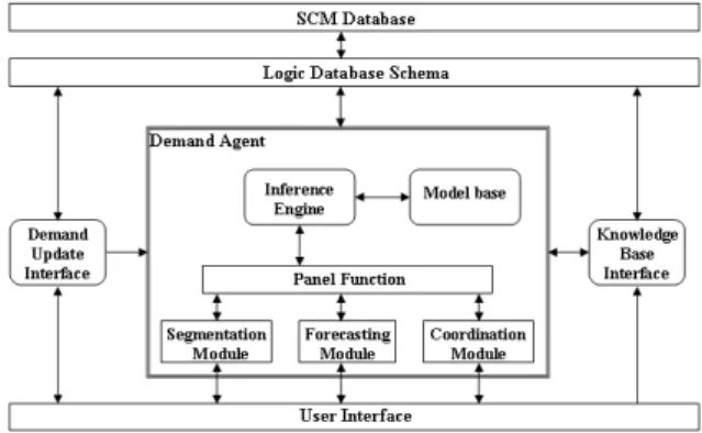
The forecasts in this section are made on one specific product in retailing industry. Figure 1 depicts the components in the presented architecture. Three of them are directly linked to user interface: Demand Update Interface, Panel Function, and Knowledge Base Interface. Behind Panel Function is Demand Agent, which drives the main process of this DSS architecture. The major effort of this study
focuses on Forecasting Module, which is the core of Panel Function.
3.1 Demand Update Interface
Demand Update Interface contains DBMS module, dealing with maintenance of SCM database, data cleaning, data preparation, and information security. Users input and update demand data through this interface.
Figure 1: Web-based architecture for demand planning
3.2 Demand Agent
Demand Agent controls Panel Function, Inference Engine, and Model Base. By the request of Panel Function, Demand Agent reads the request profile and demand data, and inactivates Inference Engine. A report is sent back to the user by Demand Agent with the result of process. Details are described in the following section.
3.2.1 Panel Function
Panel Function provides the request interface for user. When a request is proposed, Panel Function sends the request profile to Knowledge Base. If a match is found, the result is sent to Demand Agent; if not, Panel Function activates the corresponding module in it.
3.2.2 Inference Engine
The major mission of Inference Engine involves matching the request profile with knowledge base, and selecting an appropriate model in Model Base in response to the requirement by the running module. Inference Engine also makes judgment on which of the models to be chosen by request, and sends it to the client module.
3.2.3 Model Base
Model base contains models and algorithms referring to the state of the art technology. These models and algorithms are grouped as modules, and each module in them will be updated when an improved version is released.
3.3 Knowledge Base Interface
The knowledge base consists of a fact base and a rule base. The fact base stores situations and variables, while the rule base stores objectives and criteria (e.g. “what-if” rule). The Knowledge Base Interface takes charge of the maintenance of the knowledge base.
4. THE ARCHITECTURE OF
FORECASTING MODULE
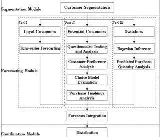
The Panel Function consists of Segmentation Module, Forecasting Module, and Coordination Module. As shown in Figure 2, the context starts from the Segmentation Module, goes on the Forecasting Module, and then terminates at the Coordination Module. This section illustrates the Forecasting Module, which is the core concept of this study.
Figure 2: Architecture of panel function 4.1 Forecasting Module
Customers in the three segments reveal different purchase behaviors, therefore different forecasting methods are applied to each segment based on the behavior pattern. ARIMA models are used in the Loyal Customer Segment for their stationary characteristics. Bayesian inference is employed for calculating each switcher's purchase probability at every promotional activity, and estimating the purchase quantity. The unknown preferences and behaviors of potential customers call for questionnaire analysis and brand choice models to obtain the purchase tendency. This purchase tendency is the key of integration function, which aims at synthesizing the analytical results from the three segments.
4.1.1 Loyal Customer Segment
Loyal customers are defined to be those who constantly purchase this product. Their purchase behavior is stable, long-term and predictable, satisfying the stationary requirement of ARIMA models. Therefore, an ARIMA model which fits the demand pattern is appropriate to predict loyal customer demand. The outcome of the forecasting is FLt, standing for the forecast value at timeperiod
t for loyal customers.
4.1.2 Potential Customer Segment
The process of mining purchase tendency includes two stages: questionnaire analysis for mining customer preferences, and quantification of these preferences with brand choice models. The preference of customers in this segment is unknown, so questionnaire analysis is needed to assist identifying the customer preference. The result of preference analysis decides what attributes to be used for estimation of utility. With selected factors, it goes on assessment of the utility function and calculation of utilities. The utilities are the foundation of estimating skewness and kurtosis, which decide the selection of a fitting choice model. The probability obtained from the selected choice model is Tp , the purchase tendency. This
estimation process is based on the approach presented by Matsatsinis and Samaras [20], and the implementation of this process is illustrated in Subsection 5.4.
4.1.3 Switcher Segment
Switchers refer to customers who only buy the specific product at promotional activities or premium price. Bayesian inference method is employed to calculate the conditional probability of customer's decision, and a total purchase quantity in the Switcher Segment is estimated. The estimated total quantity is then multiplied by the probability to obtain the Switcher forecast at time period t, FSt.
An important mission of Bayesian inference is to induce a better aggregate forecast than a stand-alone one. The evaluation of forecasting performance in this segment consists of the aggregation of Loyal Customer Segment and Switcher Segment.
4.1.4 Integration Function of Forecasting
One of the major contributions of this study is the integration function Ft, which integrates the
demand forecasts FLt, Tp, and FSt. FLt and t
FS are additive quantities, while Tp is a
probability representing a tendency. This calls for a transformation function, g(Tp), which is formulated depending on the distribution of the demand data for transforming Tp to the corresponding quantity.
The following lists the general form of integration function.
p t t t p t t f FL,T ,FS FL gT FS F ( ) (1)5. IMPLEMENTATION
The proposed architecture is designed to apply to customer database. Customers are separated into different segments based on their demographics and sales data. To give an example of how this architecture works, posted data from Monthly Report on Tourism is used to illustrate the concepts involved. 5.1 Data
In this research, inbound series of monthly tourist arrivals from Japan is retrieved from Monthly Report on Tourism (Tourism Bureau, R. O. C., 2007) from January 2001 to July 2006 for implementation in Forecasting Module. The series data, retrieved from the official website of Tourism Bureau, are public and provided by the top-level authority of tourist industry in Taiwan, and are therefore considered authentic and suffice for the purpose. Figure 4 draws the series line chart. This series, named Series Japan, lists different purposes of visiting Taiwan including Business, Pleasure, Visiting Relatives, Conference, Study, Others, and Unstated. The predominant two categories (Business and Pleasure, 88%) are selected for analysis.
Figure 3: Inbound tourist series from Japan with its sub-series business and pleasure
As stated before, in the proposed forecasting architecture different forecasting technologies are performed in accordance with the nature of the tourists in each segment. The stable nature of Series Business satisfies the stationary requirement of ARIMA, so ARIMA is applied to Series Business to simulate Loyal Customer Forecasting. Switchers are those who buy the product only at promotion activities, their behavior is event-driven. The priori probability can be calculated from their previous sales, so Bayesian inference is appropriate for predicting their future sales. Series Pleasure
fluctuates seasonally, which is associated with holidays, vacations, and promotion activities, so Bayesian inference is employed for Switcher Forecasting for the event-driven behavior of the tourists belonging to this segment. In Potential Customer Forecasting, the anticipated outcome of questionnaire analysis is shown by customer preference tables, a utility function is estimated to obtain utility values from those preference tables, and a brand choice model is selected based on the knowledge rules presented by Matsatsinis & Samaras [20]. ARIMA is also applied to Series Japan for the purpose of comparing performance with the integrated forecast. In the implementation, the training sample period is chosen from January 2001 to August 2005, while the forecasting period is from September 2005 to July 2006. The comparison of performance is based on the forecasting period, and the performance measure used for comparison is mean absolute percentage error (MAPE).
5.2 Loyal Customer Forecasting
The ARIMA ( p,d,q) model is defined as t q t d p(B)(1B)Y C(B) [1], where p p p B B B B ( ) 1 2 ... 2 1 (2) q q q B B B B ( ) 1 2 ... 2 1 (3)
B is the backshift operator, i.e. BYt Yt1, t
is the random disturbance called “white noise”,
p
indicates the number of AR parameters of ,d
is the number of times the data should be differenced to induce a stationary series,q
is the number of MA parameters of . The estimated model for Series Business in this form is then given byt t t t t t u A A Y Log Y Log Y Log 1 3 1 3 2 2 1 1 0 ( ) ( ) ) ( (4) where (1 B )(1 B )ut (1 B)(1 B15)t 15 1 15 15 2 2 , t
A is a dummy variable referring to the effect of SARS at time period t. For the purpose of adjustment, if the number of tourist arrivals is affected by SARS, then At equals to 1; otherwise,
t
A equals to 0.
The parameters of the model are estimated by statistical software EViews. Thus, Equation (3) can be rewritten as t t t t t t u A A Y Log Y Log Y Log 1 2 1 811 . 0 434 . 0 ) ( 874 . 0 ) ( 417 . 0 86 . 14 ) ( (5) where t t B B u B B )(1 0.333 ) (1 0.294 )(1 0.859 ) 393 . 0 1 ( 2 12 12
. This model fits the requirements of no autocorrelation, no serial correlation, and no heteroskedasticity. The R2 value of this model is
0.9743, which leads to the MAPE of 4.19%. Figure 4 shows the actual Series Business and estimated series.
Figure 4: Actual series business and the estimated series
5.3 Switcher Forecasting
An ARIMA model of Series Pleasure is estimated for the purpose of comparison between ARIMA and Bayesian inference, so the switcher forecasting succeeds the loyal customer forecasting in this section. The R2 value of this model is 0.9667
and the MAPE is 10.9%, revealing the need of a better fitting model for the Switcher Segment. For this reason, monthly tourist arrival ratio from September 2005 to July 2006 is calculated as the prior probability. The duration of each “event” refers to each year from 2001 to 2006, while the "time period" refers to each month from January to December. The logarithm of the total arrivals in 2006 is estimated by the equation ln
y bmxt, the parameters b13.22 , m1.004 , and 1 0.2 2 1 1 x tt xt t , for t2,3,...,6 corresponding to years 2002, 2003, …, 2006, respectively. The estimated total number of arrivals in 2006 is ye13.56774856, and monthly arrivalsfrom January 2006 to July 2006 are calculated by the ratio to the estimated total as the forecasts. The MAPE of Bayesian approach is 7.44%, which is much better than that of ARIMA model.
The aggregate forecasting performance of Series Business and Series Pleasure is also compared between Model RR and Model RB, in which Model RR is the summation of Business ARIMA forecasts and Pleasure ARIMA forecasts, and Model RB refers to the summation of Business ARIMA forecasts and Pleasure Bayesian forecasts. The MAPE calculation is based on equation (4). It is shown in Table 2 that Model RB outperforms Model RR significantly.
) s ( t t t t leasure EstimatedP s usine EstimatedB Japan (6) Table 2: Comparison performance between Mode RR
and Model RB
Model RR Model RB
MAPE 11.99 6.88
5.4 Potential Customer Choice Probability
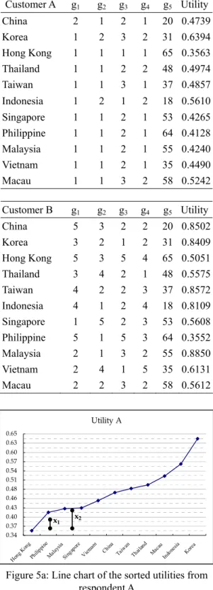
Potential customer forecasting involves complicated analysis skills. According to the process presented by Matsatsinis & Samaras [20], customer preference table is the starting point. Based on the customer preference tables, a utility function is evaluated to obtain utility values, and the parameters are assessed with these utility values. Table 3 lists two preference tables and their estimated utility values, in which equation (5) and equation (6) states their utility functions. Figure 5 depicts the line charts of the sorted utilities for respondent A and B. 1 ) ( max 1 ) ( max 082 . 0 ) 5 1 ln( ) 1 ln( 286 . 0 ) 5 1 ln( ) 1 ln( 244 . 0 ) 5 1 ln( ) 1 ln( 361 . 0 ) 5 1 ln( ) 1 ln( 027 . 0 ) ( 5 5 5 1 3 2 1 g g g g g g g g u j j j j j j j aj (7) 1 ) ( max 1 ) ( max 089 . 0 ) 5 1 ln( ) 1 ln( 669 . 0 ) 5 1 ln( ) 1 ln( 068 . 0 ) 5 1 ln( ) 1 ln( 045 . 0 ) 5 1 ln( ) 1 ln( 130 . 0 ) ( 5 5 5 4 3 2 1 g g g g g g g g u i j i j j j j bj (8)
The assessment of parameters involves the calculation of skewness 3, kurtosis 4, and the
judgment of . By definition, 3 2 3 3m m and 3 ) ( 2 2 4 4 m m , where
1 1 1 1 ( ) n i i n i r i i r f x f m and
1 1 1 1 n i i n i i i f x f .
is the mean value of the frequenciesof arrival, and fi ni n is the frequency of arrivals
in interval xi. The value of is determined by the range RUmaxUmin as follows: 1 if
1 . 0 0R ; 2 if 0.1R0.3 , 3 if 6 . 0 3 . 0 R , and 4 if 0.6R1. Table 4 shows the variables of estimation of 3 and 4.
A choice model is then selected from Table 5 as a result of mapping the parameters with the knowledge rules in Appendix A. The choice probability is calculated from the selected choice model. When the probabilities for all destinations
are yielded, the averaged probability for a specific destination is calculated to be the parameter of estimating the number of potential customers in integration function. Table 6 lists the obtained parameters, the selected choice model, the probabilities for each customer, and the averaged choice probability.
Table 3: Two multicriteria preference tables and utilities of overseas travelers from Japan Customer A g1 g2 g3 g4 g5 Utility China 2 1 2 1 20 0.4739 Korea 1 2 3 2 31 0.6394 Hong Kong 1 1 1 1 65 0.3563 Thailand 1 1 2 2 48 0.4974 Taiwan 1 1 3 1 37 0.4857 Indonesia 1 2 1 2 18 0.5610 Singapore 1 1 2 1 53 0.4265 Philippine 1 1 2 1 64 0.4128 Malaysia 1 1 2 1 55 0.4240 Vietnam 1 1 2 1 35 0.4490 Macau 1 1 3 2 58 0.5242 Customer B g1 g2 g3 g4 g5 Utility China 5 3 2 2 20 0.8502 Korea 3 2 1 2 31 0.8409 Hong Kong 5 3 5 4 65 0.5051 Thailand 3 4 2 1 48 0.5575 Taiwan 4 2 2 3 37 0.8572 Indonesia 4 1 2 4 18 0.8109 Singapore 1 5 2 3 53 0.5608 Philippine 5 1 5 3 64 0.3552 Malaysia 2 1 3 2 55 0.8850 Vietnam 2 4 1 5 35 0.6131 Macau 2 2 3 2 58 0.5612 Utility A 0.34 0.37 0.40 0.43 0.46 0.48 0.51 0.54 0.57 0.60 0.63 0.65 Hong Kon g Philip pine Malay sia Sing apor e Vietnam Ch ina Taiw an Thail and Mac au Indo nesia Korea x1 x2
Figure 5a: Line chart of the sorted utilities from respondent A Utility B 0.33 0.38 0.43 0.49 0.54 0.59 0.65 0.70 0.75 0.81 0.86 Philip pine Hong Kong Thail and Singa pore Maca u Vietn am Indo
nesia KoreaChinaTaiwan Malay
sia
Figure 5b: Line chart of the sorted utilities from respondent B
Table 4: Necessary parameters for assessing skewness and kurtosis coefficients
A B A B Umax 0.6394 0.8850 x1 0.3987 0.4346 Umin 0.3563 0.3552 x2 0.4271 0.4876 R 0.2831 0.5299 x3 0.4554 0.5406 δ 2 3 x4 0.4837 0.5936 m2 0.0046 0.0303 x5 0.5120 0.6466 m3 0.0002 -0.0003 x6 0.5403 0.6996 m4 0.0001 0.0013 x7 0.5686 0.7526 μ 0.5068 0.7188 x8 0.5969 0.8056 x9 0.6252 0.8585 x10 0.6536 0.9115 A B f1 0.0909 0.0909 f2 0.0000 0.0000 f3 0.2727 0.0909 f4 0.0909 0.2727 f5 0.2727 0.0909 f6 0.0909 0.0000 f7 0.0000 0.0000 f8 0.0909 0.0000 f9 0.0000 0.0909 f10 0.0909 0.3636 5.5 Integrated Forecasting
The Integration function is the ultimate decision mechanism of the integrated forecast. It consists of the aggregate forecast by Model RB, and the transformation function of the choice probability. The general form of integration function is represented by equation FtFLtFStg
Tp , whereFtis the integrated forecast, FLt is the loyal customer forecast, FSt is the switcher forecast, and g(Tp)
the transformation function of choice probability Tp.
t t FS
FL refers to the aggregate forecast by Model RB, g(Tp) transforms the choice probability to a
t p
p T B
T
g( ) , where Bt is the potential customer
base. The group of Japanese overseas travelers who visited Asian countries except Taiwan is the population of potential customers. A proportion is assumed that some of these travelers ranked Taiwan as their first priority, but the tour is not carried out for some reason. Thus Bt is estimated by equation
t t t t t Asia TW TW Asia
B , where Asiat is the total
travelers to all Asian countries at time period t, and
t
TW is the number of travelers to Taiwan at time period t. The detailed integration function can be represented by equation (7), which is called Model RBP.
t t t t p st lt t Asia TW TW Asia T F F F (9)Table 5: Formula of brand choice models Brand Choice Model Formula Luce
C k ik ij ij U U C P Lesourne
C k ik ij ij U U C P 2 2 Multinomial Logit Model (McFadden-1)
C k U U ij ik ij e e C P Slightly Reinforced (McFadden-2)
C k U U ij ik ij e e C P 2 2 Width of Utilities-1
C k U U ik U U ij ij U U C P min max min max Width of Utilities-2
C k U U U U U U ij ik ij e e C P ( ) ) ( min max min max Maximum of Utilities
, U U U m C j Pij j i otherwise 0 , if 1 max max where 1 min max n U U i Equal Probabilities , where 0.1 1 min max U U m Pj* Source: Matsatsinis and Samaras [20]
Table 6: Parameters, selected choice models, and averaged choice probability
3 4 Model Probability Average A 2 0.6453 -0.0903 3 0.0925 B 3 -0.0613 -1.5907 3 0.0933 0.0929
For the purpose of comparing the performance of different approaches, ARIMA is applied to Series
Japan, represented by Model AJ. The comparison summarized in Table 7 shows that Model RB outperforms Model AJ, while Model RBP outperforms Model RB. This result verifies the effectiveness of the integrated forecasting approach.
Table 7: Comparison of performance between integrated forecasting and others
Model AJ Model RB Model RBP
MAPE 8.02 6.88 4.46
6. DISCUSSION AND
CONCLUSION
Ineffective demand planning in SCM leads to serious problems such as the bullwhip effect and severe inventory problems, a web-based DSS architecture is proposed in this study for providing more effective and accurate forecasts which may improve the demand planning performance, as well as facilitate collaborative forecasting in a supply chain with efficient collaboration mechanism.
6.1 Integrated Forecasting Strategy
In the proposed architecture, customers are divided into three different groups: Loyal Customer Segment, Potential Customer Segment, and Switcher Segment. ARIMA models are applied to the Loyal Customer Segment for estimating a time-series forecast, questionnaire and brand choice models are performed in the Potential Customer Segment to obtain customer purchase tendency, and Bayesian inference is employed in the Switcher Segment to evaluate the purchase quantities at promotional activities. The integration function integrates these analytical results to obtain an integrated forecast, which is anticipated to mitigate the forecasting error. 6.2 Research Implications
As depicted in Figure 1, the presented architecture provides a web mechanism for collaboration between supply chain members, it involves internet information technology. This study emphasizes on the forecasting core, namely Panel Function. Among the modules in Panel Function, Forecasting Module is the core of this study. In the following subsections 6.2.1 to 6.2.4, the implications of each segment and the integration function are discussed.
6.2.1 Loyal Customer Forecasting
In the Loyal Customer Segment, the MAPE of the estimated model for Business is 4.19%, while that for Pleasure is 10.9%, indicating the excellent work of the estimated ARIMA model with the dummy variable At . The ARIMA model performs
outstandingly on stationary series, and At helps capture the outliers formed by SARS effectively. 6.2.2 Potential Customer Forecasting
Potential customer forecasting is unique for its feature of mining. The process illustrated in Subsection 5.4 is designed for uncovering customer tendency. The purchase tendency represents customer inclination on the specific product, it also servers as the base of potential customer forecasting, pointing out a direction for demand planning. The important implication of this purchase tendency is that it quantifies what is inside a customer's mind and indicates a trend of customer preference, which provides a leading view of demand planning, this may help practitioners avoid mislead investment. This is the major difference of this presented forecasting method from traditional forecasting models.
6.2.3 Switcher Forecasting
Switchers purchase only at promotional activities or premium prices, making the switcher demand a non-stationary series, which explains part of the forecasting error. Bayesian inference outperforms ARIMA in the Switcher Segment on both stand-alone Series Pleasure and aggregate series of Business and Pleasure, which proves Bayesian inference a more effective approach to predict event-driven purchase behavior.
6.2.4 Integration Function
The Forecasting Module presented in this study starts from performing different analysis and forecasting processes in each segment, and ends up at integration function of integrating the analytical results from the three segments. The expected contribution of integration function is a more accurate forecast to promote demand planning performance. The implementation result listed in Table 7 reveals marvelous improvement of integrated forecasting in comparison with the straight ARIMA approach, and the hybrid model of ARIMA and Bayesian inference. The implication of this result points out a different direction from traditional linear forecasting thinking: differentiation in different customer segments should be considered in forecasting analysis. It is anticipated working effectively on promoting demand forecasting accuracy. Furthermore, the influence from qualitative factors such as customer purchase tendency should be dug out and accommodated in the forecasting model to reduce the unpredictable error. 6.3 Research Limitations
A technological limitation is that the implementation of the presented web-based DSS
might take years of expert teamwork effort, although the output will prove it worthwhile in the long run. 6.4 Conclusion and Future Research
Demand planning is the key factor of lowering down inventory level and gaining maximum profit in SCM. In the past, time-series forecasting models, the classical methods for demand forecasting, assume time series as a linear series containing all the information needed to forecast the future, and this makes a problem when they are applied to a nonlinear series. Forecasting Module, the core of this architecture, is designed to work out this problem by mining customer purchase tendency with their preference. The proposed web-based DSS architecture is designed to help unloose the obstruction of information caused by information sharing deficiencies. This architecture is quite complicated but worth implementation for its effectiveness, it facilitates collaborative forecasting and benefits quick response in a supply chain.
The proposed web-based DSS is a first stone of web-based integrated forecasting system, pointing out an optimistic direction of improving forecasting technology. Boundless development may be done by future effort in this architecture. Some possible future researches are: (1) applying Fuzzy to seize customer preference in comparison with brand choice models (2) analyzing switchers' choice behavior with brand choice models. This might lead to a deeper behavioral analysis. (3) estimating potential customer base with different approaches and variables. For instance, economic prosperity might be an important index of potential customer base.
In this study the result of integration function provides a managerial implication of planning cost: a rough segmentation of sub-series may achieve a satisfactory performance, indicating better performance with precise segmentation. It is a trade-off between better performance and lower planning cost.
Also, it is interesting to decipher what influences the decision process behind purchase behavior and how to measure it in a managerial architecture. The Potential Customer Forecasting is an attempt to quantify the qualitative inside tendency, and provides it as a foundation of quantitative integration forecasting. The implementation results show that the proposed integrated forecasting core effectively mitigates forecasting error, indicating an optimistic direction. Further research toward this direction could make the integrated forecasting technology fruitful.
REFERENCES
1. Box, G. E. P., Jenkins, G. M. and Reinsel, G. C., 1994, Time Series Analysis: Forecasting & Control, Prentice Hall, New Jersey.
2. Fredenhall, L. and Hill, E., 2001, Basics of Supply Chain Management, St. Lucie Press, New York.
3. Ghiassi, M. and Spera, C., 2003, “Defining the internet-based supply chain system for mass customized markets,” Computers & Industrial Engineering, Vol. 45, No. 1, pp. 17-41. 4. Ghiassi, M., Saidane, H. and Zimbra, D. K.,
2005, “A dynamic artificial neural network model for forecasting time series events,” International Journal of Forecasting, Vol. 21, No. 2, pp. 341-362.
5. Gunasekaran, A. and Ngai, E. W. T., 2004, “Information systems in supply chain integration & management,” European Journal of Operational Research, Vol. 159, No. 2, pp. 269-295.
6. Ha, S. H., Bae, S. M. and Park, S. C., 2002, “Customer’s time-variant purchase behavior and corresponding marketing strategies: An online retailer’s case,” Computers & Industrial Engineering, Vol. 3, No. 4, pp. 801-820. 7. Hsieh, N. C., 2004, “An integrated data mining
and behavioral scoring model for analyzing bank customers,” Expert Systems with Applications, Vol. 27, No. 4, pp. 623-633.
8. Hwang, H. S., Jung. T. S. and Suh, E. H., 2004, “A LTV model and customer segmentation based on customer value: A case study on the wireless telecommunication industry,” Expert Systems with Applications, Vol. 26, No. 2, pp. 181-188.
9. Jeong, B., Jung, H. S. and Park, N. K., 2002, “A computerized causal forecasting system using genetic algorithms in supply chain management,” The Journal of Systems and Software, Vol. 60, No. 3, pp. 223-237.
10. Keogh, E. and Kasetty, S., 2002, “On the need for time series data mining benchmarks: A survey and empirical demonstration,” The 8th ACM SIGKDD International Conference on Knowledge Discovery and Data Mining, http://citeseer.ist.psu.edu/keogh02need.html. 11. Kuo, R. J., Wang, H. S., Hu, T. L. and Chou, S.
H., 2005, “Application of ant K-means on clustering analysis,” Computers and Mathematics with Applications, Vol. 50, No. 10-12, pp. 1709-1724.
12. Last, M., Klein, Y. and Kandel, A., 2001, “Knowledge discovery in time series databases,” Proceedings of IEEE Transactions on System, Man, and Cybernetics Part B:
Cybernetics, Vol. 31, No. 1, pp. 160-169. 13. Lee, H. L., Padmanabhan, V. and Whang, S.,
1997, “The bullwhip effect in supply chains,” Sloan Management Review, Vol. 38, No. 3, pp. 93-102.
14. Lee, J. H. and Park, S. C., 2005, “Intelligent profitable customers segmentation system based on business intelligence tools,” Expert Systems with Applications, Vol. 29, No. 1, pp. 145-152.
15. Lee, S. C., Suh, Y. H., Kim, J. K. and Lee, K. J., 2004, “A cross-national market segmentation of online game industry using SOM,” Expert Systems with Applications, Vol. 27, No. 4, pp. 559-570.
16. Liao, S. H. and Chen, Y. J., 2004, “Mining customer knowledge for electronic catalog marketing,” Expert Systems with Applications, Vol. 27, No. 4, pp. 521-532.
17. Lingras, P., Hogo, M., Snorek, M. and West, C., 2005, “Temporal analysis of clusters of supermarket customers: Conventional versus interval set approach,” Information Science, Vol. 172, No. 1-2, pp. 215-240.
18. Manrai, A. K., 1995, “Mathematical models of brand choice behavior,” European Journal of Operational Research, Vol. 82, No. 1, pp. 1-17. 19. Martino, J. P., 2003, “A review of selected
recent advances in technological forecasting,” Technological Forecasting and Social Change, Vol. 70, No. 8, pp. 719-733.
20. Matsatsinis, N. F. and Samaras, A. P., 2000, “Brand choice model selection based on consumers’ multicriteria preferences and experts’ knowledge,” Computers & Operations Research, Vol. 27, No. 7-8, pp. 689-707. 21. Patterson, K. A., Grimm, C. M. and Corsi, T.
M., 2003, “Adopting new technologies for supply chain management,” Transportation Research, Vol. 39, No. 2, pp. 95-121.
22. Peng, Y. Q., Zhang, Y. and Tian, H. S., 2003, “Research of time series pattern finding based on artificial neural network,” The Second International Conference on Machine Learning and Cybernetics, pp. 1385- 1388.
23. Rhee, H. and Bell, D. R., 2002, “The inter-store mobility of supermarket shoppers,” Journal of Retailing, Vol. 78, No. 4, pp. 225-237.
24. Shim, J. P., Warkentin, M., Courtney, J. F., Power, D. J., Sharda, R. and Carlsson, C., 2002, “Past, present, and future of decision support technology,” Decision Support Systems, Vol. 33, No. 2, pp. 111-126.
25. Strader, T. J., Lin, F. R. and Shaw, M. J., 1998, “Information infrastructure for electronic virtual organization management,” Decision Support Systems, Vol. 23, No. 1, pp. 75-94. 26. Thomas, J., 1999, “Why your supply chain
doesn’t work,” Logistics Management and Distribution Report, Vol. 38, No. 6, pp. 42-44. 27. Wang, X. Y. and Wang, Z. O., 2002, “Stock
market time series data mining based on regularized neural network and rough set,” The First International Conference on Machine Learning and Cybernectics, Beijing, China, pp. 315-318.
ABOUT THE AUTHORS
Tien-You Wang is an Associate Professor in the Department of International Business Management at Tainan University of Technology (TUT), Taiwan. She received her Ph.D. degree in Business Administration at National Chung Cheng University in 2006. Her research interests are integrating IT and demand planning related technologies in Supply Chain Management. In particular, she is interested in data mining, neural network, and time series forecasting. Din-Horng Yeh is an Associate Professor in the Department of Business Administration at National Chung Cheng University (CCU), Taiwan. His research interests are Queuing and Simulation.
(Received November 2007, revised March 2008, accepted May 2008)
Appendix A
The Rule Base of Choice Model
Selection
Notation:
, 3, 4: category of utility, skewness,
kurtosis.
Model: the model number in Table 5.
Rule 1
if
= 1 then Model = 8 Rule 2if = 2 and (3≧-0.25 and 3≦0.25) and 4
< -0.5 then Model = 1 Rule 3
if = 2 and (3≧-0.25 and 3≦ 0.25) and
(4≧-0.5 and 4≦0.5) then Model = 2
Rule 4
if = 2 and (3≧-0.25 and 3≦0.25) and 4
> 0.5 then Model = 3 Rule 5
if = 2 and 3> 0.25 and 4< -0.5 then Model
= 2
Rule 6
if = 2 and 3> 0.25 and (4≧-0.5 and 4
≦0.5) then Model = 3 Rule 7
if = 2 and 3> 0.25 and 4> 0.5 then
Model = 4 Rule 8
if = 2 and 3< -0.25 and 4< -0.5
then Model = 3 Rule 9
if = 2 and 3< -0.25 and (4≧-0.5 and 4
≦0.5) then Model = 4 Rule 10
if = 2 and 3< -0.25 and 4> 0.5 then
Model = 5 Rule 11
if = 3 and (3≧-0.25 and 3≦0.25) and 4
< -0.5 then Model = 3 Rule 12
if = 3 and (3≧-0.25 and 3≦0.25) and
(4≧-0.5 and 4≦0.5) then Model = 4
Rule 13
if = 3 and (3≧-0.25 and 3≦0.25) and 4
> 0.5 then Model = 5 Rule 14
if = 3 and 3> 0.25 and 4< -0.5 then
Model = 2 Rule 15
if = 3 and 3> 0.25 and (4≧-0.5 and 4
≦0.5) then Model = 3 Rule 16
if = 3 and 3> 0.25 and 4> 0.5 then
Model = 4 Rule 17
if = 3 and 3< -0.25 and 4< -0.5 then
Model = 4 Rule 18
if = 3 and 3< -0.25 and (4≧-0.5 and 4
≦0.5) then Model = 5 Rule 19
if = 3 and 3< -0.25 and 4> 0.5 then
Model = 6 Rule 20
if = 4 and (3≧-0.25 and 3≦0.25) and 4
< -0.5 then Model = 3 Rule 21
if = 4 and (3≧-0.25 and 3≦0.25) and
(4≧-0.5 and 4≦0.5) then Model = 5
Rule 22
if = 4 and (3≧-0.25 and 3≦0.25) and 4
Rule 23
if = 4 and 3> 0.25 and 4< -0.5 then
Model = 5 Rule 24
if = 4 and 3> 0.25 and (4≧-0.5 and 4
≦0.5) then Model = 6 Rule 25
if = 4 and 3> 0.25 and 4> 0.5 then
Model = 7 Rule 26
if = 4 and 3< -0.25 and 4< -0.5 then
Model = 6 Rule 27
if = 4 and 3< -0.25 and (4≧-0.5 and 4
≦0.5) then Model = 7 Rule 28
if = 4 and 3< -0.25 and 4> 0.5 then
Model = 7
供應鏈需求預測之網際決策支援系統架構
王天祐
*
、葉丁鴻
*
台南科技大學國際企業經營系
台南縣永康市中正路
529
號
國立中正大學企業管理系
嘉義縣民雄鄉大學路
168
號
摘要
在現今競爭激烈的市場環境下,供應鏈管理已成為企業生存的關鍵因素。而在供應鏈 管理之中,需求規劃又扮演了極重要的角色,因為正確的需求預測能提供降低存貨水 準、縮短前置時間、進行有效的資源配置,以及迅速回應顧客需求的諸多益處,來讓 顧客滿意。為了尋求更精確的需求預測結果,本研究提出了一套內含預測核心的網際 決策支援系統,期待藉由針對不同特性顧客族群個別預測、再整合族群預測結果的方 式,來達到提昇預測正確率的功效。該預測核心先以市場區隔技術,將顧客分為三項 群組:忠誠顧客,潛在顧客,以及投機顧客;在這三項族群中分別以適當的預測技術 進行預測,再將個別預測結果加以整合,以達到最佳成效。忠誠顧客購買行為有一定 規律,適合以時間數列預測;投機顧客指有優惠活動時才出手購買的消費者,對於消 費行為的預測須借重其歷史資料中的購買行為模式,因此採用貝氏推論法由事前機率 來估計。潛在顧客需靠問卷及品牌選擇模式來分析消費者心中的購買傾向,來預測其 購買機率,再整合潛在顧客基底轉換成預測量。這三項群組的預測完成後,整合函數 便將這些預測結果加以整合。實證結果證明,此預測核心比傳統需求預測技術的績效 更好,明顯降低了預測誤差率;而此決策支援系統架構則提供了供應鏈管理中有效的 協作機制,使供應鏈成員能透過該機制迅速進行溝通協調,並以預測核心所提供的高 效能預測結果,有效達成協同預測的目的。 關鍵詞:網際決策支援系統、預測、購買傾向、整合預測、資料探勘 (*聯絡人:[email protected])